Interface Separation Detection of Concrete-Filled Steel Tube Using a Distributed Temperature Measuring System

Abstract

In recent years, concrete-filled steel tubular (CFST) bridges have been widely used in bridge construction. However, interface disengaging is one of the bridges’ most common defects. It affects not only the confinement of the steel tube to the core concrete, but also the bearing capacity and the structure durability. In order to solve the problem of disengaging at the interface of steel tube-confined concrete and ensure the integrity of the structure, a new method based on a distributed temperature detection system is proposed to identify disengaging at the interface between steel tube and concrete. Through the analysis of experiments and numerical simulation, it was found that when the structure surface was heated, the temperature of the void area was higher than that of the solid area. The temperature of the maximum void height was the highest, the temperature increase rate was the fastest, and the cooling rate was the slowest. The boundary of the void suffered from sudden changes in temperature. The more serious the void, the greater was the temperature difference between the void and the solid. After changing the heating direction, the temperature distribution could still be identified. This study achieved simplicity and efficiency with respect to the detection of interface separation.

1. Introduction

Concrete-filled steel tubular (CFST) arch bridges have been widely used in recent decades at home and abroad, and have been studied in the United States, France, Spain, and Japan. Most of the CFST arch bridges are exposed to the natural environment’s conditions, and many bridges are in an extremely bad environment, likely damaged by acid or alkaline materials. According to previous investigations [1,2], the most common problem of the concrete-filled steel tube arch rib is the interface void between the concrete and the steel tube. This problem is highly concealed and presents a very serious risk of harm, which directly affects the safety of concrete-filled steel tube arch bridges during operation [3,4,5].

Many research results show that an interface void is inevitable, especially in the vault. The main causes of the interface void are construction technology, gravity drop, temperature change, and concrete shrinkage. The existence of an interface void makes the structure lose the hoop effect of steel tube on concrete, and reduces the bearing capacity of the arch rib. As the void height and scope increase, the bearing capacity decreases even more.

Existing nondestructive tests of CFST arch bridges with disengaging at the steel–concrete interface include surface wave detection [6,7], partial quantitative self-excitation method [8], ultrasonic testing [9], optical fibers detection [10], infrared thermography [11], and so on [12,13].

Surface wave detection is based on a spectral variation mechanism of transmitted pulse reacting to the degree of defect [14]. The advantage of detection is a fast testing speed and a relatively low cost. However, this technique is not mature and still at the stage of laboratory experiments.

The partial quantitative self-excitation method applies an incentive to the structure through a hammer. The interface separation can be identified from the spectrum calculated by the time domain signals [15,16]. This method is simple and easy to be integrated, but it is hard to conduct boundary recognition.

Ultrasonic testing is one of the most widely used nondestructive testing methods. It can speculate the defects within the concrete through ultrasonic detectors and transducers. Measurements such as first wave amplitude, propagation velocity, and the main frequency of receipt signal are analyzed [17,18]. The testing results are relatively reliable, and the procedures are simple. However, this method can only detect defects quantitatively.

Optical fibers detection embeds sensing fiber in concrete during construction. The defects in bonding interface may cause the micro-bending of optical fibers. Defects in concrete can be detected through the consumption of the optical transmission and the change of the mode coupling characteristics of the optical fiber [19,20]. The limitation of this approach is that it can only be applied to newly built bridges.

Infrared thermography is a main method used in CFST nondestructive testing, which is based on the theory of heat transfer. The temperature distribution on the structure surface measured by a thermal imager is used to detect the defects [21,22,23,24,25]. However, the results of infrared radiation are influenced by factors like surface material and surroundings.

In the research of nondestructive testing and monitoring technology for the interface void of concrete-filled steel tube arch bridges, much research at home and abroad has been focused on qualitative detection technology. Most of these methods are related to point detection, with a small detection range, expensive equipment and a huge volume. These factors make it impossible to carry out real-time monitoring of the interface voids of existing CFST arch bridges.

The core issue of the damage evolution law of bridge engineering is “damage identification and location”. Based on an understanding of the local key points, through damage identification and quantitative testing to provide direct and reliable information for a structural safety assessment, and to effectively save the cost of sensor placement, these are the key points to consider when monitoring the voids of concrete-filled steel tube arch bridges over the long term.

Therefore, this paper proposes a new method of nondestructive testing and long-term monitoring of concrete-filled steel tube based on distributed temperature measurement, in order to form a set of effective and convenient detection monitoring systems for the nondestructive testing of concrete-filled steel tube. This method is simple, and the cost is relatively low. It could also be used for boundary recognition, and its limitations are minor.

2. Methodologies

2.1. Principle

It is well known that the thermo-physical properties of solid and gas are different. As shown in Table 1 and Table 2 [26,27], the thermal conductivity of air is less than that of steel and concrete by approximately 70–2000 times. Therefore, significant differences exist in the temperature field of different void forms in concrete-filled steel tubes. Moreover, with the increase of void area, the differences are more evident.

Table 1. Thermo-physical properties of steel and concrete.

Material Properties (20 °C)	Density (kg/m3)	Specific Heat (J/kg·K)	Thermal Conductivity (J/m·K)
Steel	7833	465	54
Concrete	2344	750	1.84

Table 2. Thermo-physical properties of air under different temperatures.

Temperature (°C)	20	30	40	50	60	70
Density (kg/m3)	1.205	1.165	1.128	1.093	1.060	1.029
Thermal conductivity (W/m·K)	0.0259	0.0267	0.0276	0.0283	0.0290	0.0296
Specific heat (J/kg·K)	1005	1005	1005	1005	1005	1009

2.2. Numerical Validation

In order to validate the feasibility of the proposed approach on interface void detection using distributed temperature sensors, numerical models were established using the finite element software FLUENT12.0 (Version released by 28 November 2009 of American ANSYS company) [28,29,30], which is widely used to solve fluid problems.

2.2.1. Model Building

Three CFST models were designed as shown in Table 3. Model 1, as a comparison, did not contain a void area, Model 2 was created with a 2.5 cm cavity, and Model 3 was created with a cavity height of 5.0 cm. The outer diameter of the steel tubes was 273 mm, and the wall thickness was 8 mm. The steel tubes were filled with C50 concrete. The outer surface of the steel pipe’s upper semicircle was the temperature load inlet, and the load form was set to the boundary of the constant heat flux. The heat flux was 800 W/m². Based on the literature regarding the temperature field analysis of concrete-filled steel tube and the temperature detection data of some bridges, it was found that the arch rib’s temperature could reach above 50 °C under sunshine. This value could make the structure close to the actual temperature that the authors expected to reach after heating. The outer surface of the lower semicircle was set to the outlet. It could exchange heat with the outside and the heat transfer coefficient was 8.7 W/(m²·K). The two ends of the cylinder were defined as the adiabatic boundary without taking into account the influence of this part, because it was only a small section of the whole concrete-filled steel tube structure. There were three possible boundary contacts in the interior: the contact between steel tube and concrete, the contact between steel tube and air, and the contact between air and concrete. All boundary conditions were set to coupled wall. Convection heat transfer was carried out between them. Considering the influence of the heating position in the actual environment, the heating surface was rotated counterclockwise 30°, 45°, 60°, and 90° for the simulations. The specific location of the heating surface is shown in Figure 1.

Table 3. Size of specimens.

Number	Diameter(mm)	Wall Thickness (mm)	Length (mm)	Cavity Height (mm)	Concrete Strength
1	273	8	300	0	C50
2	273	8	300	25	C50
3	273	8	300	50	C50

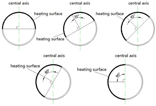
Figure 1. Different heating directions of the model.

The initial temperature was assumed to be 20 °C. The parameters of the thermo-physical properties of the different materials are shown in Table 1. The form of heat transfer was set to unsteady heat transfer and the k-epsilon equation was used to calculate. The computation time was 1800 s.

2.2.2. Results and Analysis

Model 1

As shown in Figure 2, the temperature of the section in Model 1 was a ladder-like distribution according to heating position and sectional form. The temperature isograms distributed more densely when the position was closer to the heating surface, and more sparsely when it was far away from the heating surface. The isotherm behaved like a circular arc protruding toward the heating surface. The temperature of the section decreased along the circular arc. The highest temperature at the top of the model was approximately 311.75 K, whereas the lowest temperature was 294.95 K at the bottom of the model.

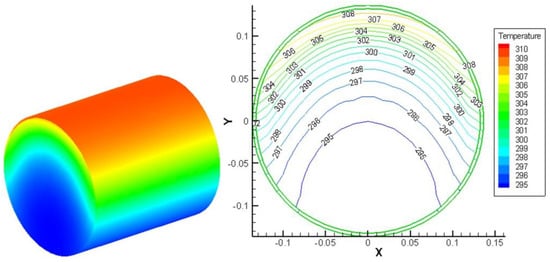
Figure 2. Temperature cloudy map and isopleth in Model 1 (unit: K).

Model 2

The temperature field of the solid section in Model 2 is illustrated in Figure 3. Unlike the solid Model 1, there was a sudden temperature change in the interface of the void. The isotherm was no longer like a circular arc. The maximum temperature at the top of the section was as high as 327.75 K, but the temperature at the bottom was only approximately 295.05 K, which was almost identical to that in Model 1. Because of the void’s existence, the maximum temperature at the top of the model had significantly increased. The highest temperature difference was 16 K higher than in Model 1, and the lowest temperature rose by nearly 0.1 K.

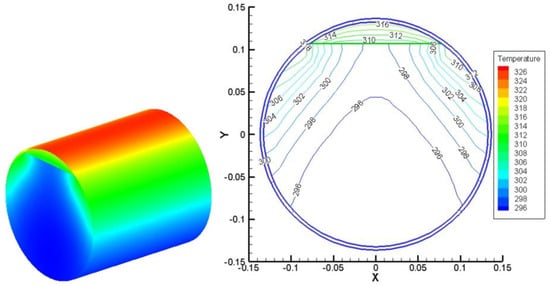
Figure 3. Temperature cloudy map and isopleth in Model 2 (unit: K).

Model 3

The temperature distribution of Model 3 was similar to that of Model 2. Both had a sudden temperature change at the interface of the void. As can be seen in Figure 4, with the increase of the void height, the difference in temperature became more evident on both sides of the interface and the temperature at the top of the model increased even more. The maximum temperature at the top was 334.15 K, and the lowest one at the bottom was 295.25 K. The highest temperature when comparing it with Model 1 and Model 2 increased by 22.4 K and 6.4 K, whereas the lowest temperature increased by 0.3 K and 0.2 K, respectively.

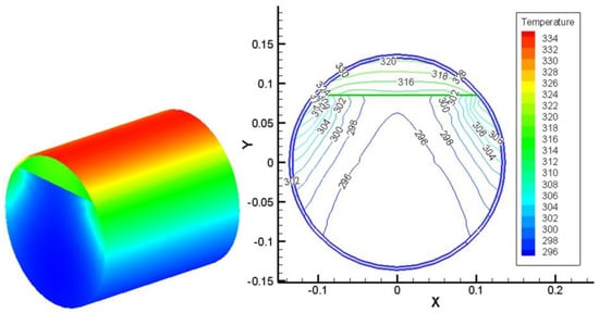
Figure 4. Temperature cloudy map and isopleth in Model 3 (unit: K).

The temperature distribution under different heating angles is shown in Figure 5, Figure 6, Figure 7 and Figure 8. For comparison, all models were simulated based on a void height of 25 cm. It was observed that although the heating angle had changed, the high temperature area of the concrete-filled steel tube structure was still concentrated in the void section. The temperature distribution on the surface of the model was no longer symmetrical as the heating direction shifted. The temperature of the left side was gradually higher than the right side. The distribution of isotherms in the void area was dense, but the distribution of isotherms in the solid part was sparse, with stepped distribution characteristics. There was also an obvious temperature change at the interface of the voids. Although the temperature difference of the right side was smaller than that of the initial heating direction, it was still possible to identify. As in the case of the 90° anticlockwise rotation, the sudden temperature change on the right side was the smallest. Furthermore, the whole temperature distribution of the model was completely different from the complete structure.

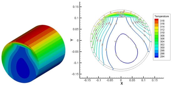
Figure 5. Temperature cloudy map and isopleth at 30° (unit: K).

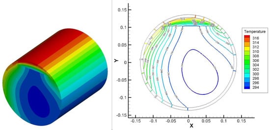
Figure 6. Temperature cloudy map and isopleth at 45° (unit: K).

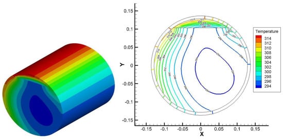
Figure 7. Temperature cloudy map and isopleth at 60° (unit: K).

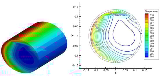
Figure 8. Temperature cloudy map and isopleth at 90° (unit: K).

2.3. Experimental Validation

As explained in this section, the experimental results were built as a reference to compare the consistency with numerical models. A laboratory experiment was carried out at the Dalian University of Technology & Bridge Research Base. To avoid the natural environment’s influence, an artificial heat source was used instead of a solar heat source. First, CFST specimens with different voids were heated in the laboratory and then the temperature data of the specimens were collected. Differences in the temperature distribution between the void and the solid CFRT were compared.

2.3.1. Experimental Scheme Design

The size of the specimens was the same as the experimental models shown in Table 3. In addition, the numbering of the specimens corresponded to a pairwise comparison of the models (e.g., Specimen 1 corresponded to Model 1). An expansion agent was added to the concrete to ensure its tightness. As shown in Figure 9, temperature sensors were placed around the middle of the CFRTs, which reduced the influence of axial external media. Point 1 was arranged at the same position of the three models to compare the effect of the temperature on specimens with a different cavity height. Points 2 and 3 were arranged at the same position of Models 1 and 2 to compare differences in the temperature distribution between the void and solid specimens. In order to study how to identify the void area accurately, measuring points were arranged at both sides of the boundary’s separation region. Considering the heating direction’s influence, two heating modes were investigated for Specimen 2, as shown in Figure 10.

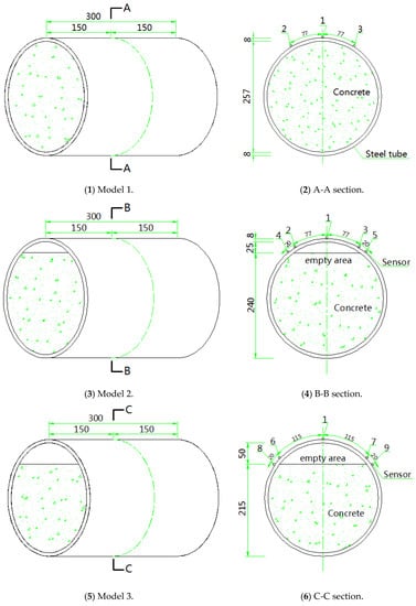
Figure 9. Specimen size and sensor layout.

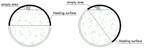
Figure 10. Heating range.

Temperature sensors used in the experiment were DS18B20 (Dallas Semi-conductor Corporation, Dallas, TX, USA) with a working temperature range of 0–50 °C, which were matched with a STA-D data acquisition module. This data acquisition module can receive a signal remotely, and the effective temperature range is −55 °C to +125 °C with a measure error of 0.1 °C. Silicone heating film was used as a heating source, whose working temperature range was from 10 °C to 120 °C. The experiment was carried out in the winter season, and the installation environment was in the laboratory. Considering the heating of the specimen, the heat exchange between the concrete-filled steel tube and the outside and the room temperature, the heating temperature was set at 40 °C. The heating time of the specimen was 55 min, which was based on the results of the first experiment. The results showed that the surface temperature of the specimen had stabilized after 55 min of heating. The testing system is shown in Figure 11.

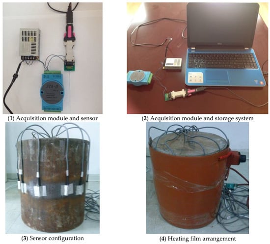
Figure 11. Testing system.

2.3.2. Experimental Procedure

Temperature sensors were pasted onto the surface of the steel tubes according to the experimental design. Then, silicone-heating film was coated onto the model’s surface to facilitate the heat flux entry. Ceramic fiber film and aluminum foil tape were used to insulate the temperature sensors to reduce the influence of the heating film on the temperature sensors. The test was carried out in accordance with the sequence described in Table 4. The temperature was recorded in the storage system. The heating time was 55 min for each experiment.

Table 4. Experimental procedure.

Experiment Number	Specimen Number	Heating Direction
①	1	upper semicircle
②	2	upper semicircle
③	3	upper semicircle
④	2	lateral heating

2.3.3. Experimental Result

Specimen-Wise Analysis

Temperature sensors were pasted onto the surface of the steel tubes according to the experimental design. Then, silicone-heating film was coated onto the model’s surface to facilitate the heat flux entry. The temperature distribution of Specimen 1 is shown in Figure 12. During the heating stage, the specimen started to warm up rapidly from room temperature (approximately 14 °C). When the temperature reached 26 °C, it stabilized and slowly rose to the maximum temperature of 27 °C. After the heating stopped at 55 min, the specimen cooled quickly and dropped to below 22 °C at 68 min.

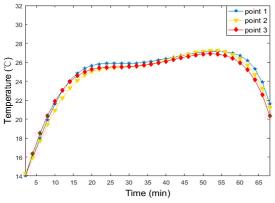
Figure 12. Temperature of each point in Experiment 1.

The temperature distribution of Specimen 2 is shown in Figure 13. points 1, 2 and 3 were located in the void area, whereas points 4 and 5 were located in the solid area. All points showed similar temperature trends.

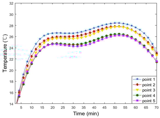
Figure 13. Temperature of each point in Experiment 2.

Affected by the height of the void, the temperature of point 1 was the highest and the temperature increase rate was the fastest. When the temperature reached 26.8 °C, the temperature increase rate decreased and slowly rose to the highest temperature of 28.1 °C. The temperature dropped to approximately 23.3 °C in 15 min during the cooling stage. The temperature distribution of points 2 and 3 were approximately equal due to symmetry. Their temperature increase rates were slightly lower than Point 1 and started to slow down at the temperature of 26 °C. The maximum temperature was 27.4 °C. It then dropped to 22.7 °C in 15 min after heating.

The temperature increase rates of points 4 and 5 were the lowest, and slowly rose to 26 °C after reaching the temperature of 24.5 °C. When heating was stopped, the temperature dropped to 21.6 °C.

This figure shows that there was a significant difference in temperature between the solid and the void areas. The mean temperature difference was 1.5 °C. Because of the existence of the void, the heat absorbed by the upper surface transferred slowly to the void area.

The temperature distribution of Specimen 3 is shown in Figure 14. At the maximum height of the void, the temperature of point 1 was the highest. It rapidly rose up to 28 °C through heating and then slowly increased to 30 °C. Because of the void’s wide range, the specimen accumulated a large amount of heat and Point 1 still maintained a high temperature for 6–7 min during the cooling stage. After 15 min, the temperature dropped to 26 °C. The temperature of points 6 and 7 were slightly lower than point 1, and the highest temperature was 29.2 °C. The position of minimum temperature was found in points 8 and 9. Heating up to 25.6 °C, the rate began to slow down and the maximum temperature could only reach 27.1 °C. The difference in temperature between the solid and the void areas was evident from this figure. The average temperature variation was more than 2 °C.

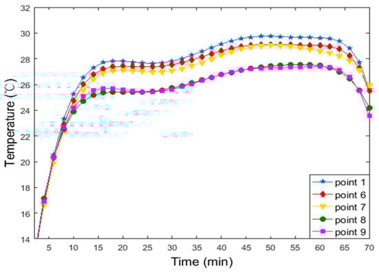
Figure 14. Temperature of each point in Experiment 3.

Changing the heating direction, the temperature distribution of Specimen 2 is shown in Figure 15. The temperature of point 1 was still the highest with the fastest rate of increase. The maximum temperature was 28 °C. The temperature dropped to 23 °C in 15 min after cooling. The temperature of points 2 and 4 located at the edge of the heating surface rose gently. The maximum temperature was 18.5 °C and 17.2 °C, respectively. Because of their low temperature, the points showed no significant cooling trend. The rising temperature trend of point 3 was similar to that of Point 5. The highest temperature was 26.7 °C and 25.6 °C, then the points cooled down to 22.5 °C and 21.8 °C, respectively.

Figure 15. Temperature of each point in Experiment 4.

Point-Wise Analysis

Figure 16 shows the temperature distribution of point 1 with different cavity heights under the same heating condition. Among them, the maximum temperature of Specimens 1–3 was 30 °C, 28.1 °C and 27 °C, respectively. Once the heating stopped, Specimens 1 and 2 began to cool immediately, whereas Specimen 3 maintained the temperature for 6 min before cooling. It is therefore clear that, when the temperature increased, the specimen temperature increased with the increasing cavity heights, and the temperature increase rate also increased. During the cooling stage, and because of the existence of the void, the temperature dropped more slowly as the volume of the void increased.

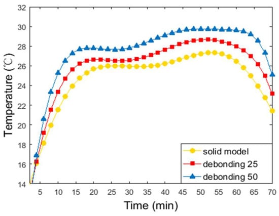
Figure 16. Temperature history of point 1.

The temperature history of the corresponding points in Specimens 1 and 2 is shown in Figure 17. The graph shows that the temperature field at points 2 and 3 was distributed symmetrically; the temperature of Specimen 2 was higher than that of Specimen 1. In the initial heating stage, the difference in temperature increase rates at point 2 was evident, having a mean temperature difference of 0.8 °C. The temperature variation at point 3 affected by the other factors was small. After heating for 30 min, the temperature difference gradually appeared, and it increased to 1.5 °C during the cooling stage.

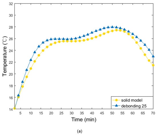
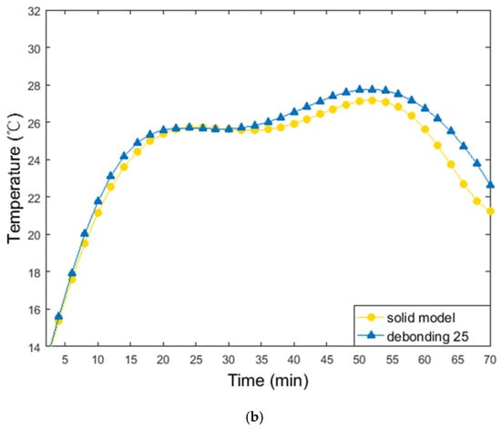
Figure 17. Temperature history of (a) point 2 and (b) point 3.

Location-Wise analysis

The temperature distribution of the void interface on both sides is shown in Figure 18. The temperature at points 2 and 3 located in the void part was higher than that at points 4 and 5 in the solid part. The difference was negligible at the beginning; however, it became significant with an average of 1.8 °C when the temperature reached approximately 24 °C. The mean temperature difference was approximately 1 °C during the cooling stage.

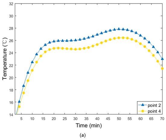
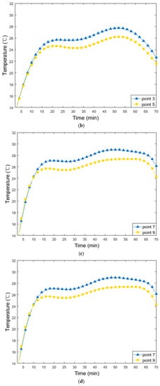
Figure 18. Temperature of the void boundary: (a,c) left side and (b,d) right side.

The temperature at points 6 and 7 located in the void part was also higher than that at points 8 and 9 in the solid part. With the increasing cavity heights, the temperature difference became larger and reached 2 °C during the heating process. During the cooling stage, the temperature remained unchanged and then decreased slowly because of the thermal storage capacity of air. The mean temperature difference was approximately 1.8 °C. It was therefore clear that the sudden change in temperature was more evident with the increasing cavity heights.

Location-Wise Analysis Under Lateral Heating

The temperature distribution of the void boundary under lateral heating is shown in Figure 19. Although the heating direction had changed, the sudden change in temperature still existed. The left side of the interface was located at the edge of the heating surface, so that the temperature of points 2 and 4 rose slowly. However, the average difference in temperature (1.8 °C) was much larger than that of points 3 and 5, which was approximately 1 °C during the heating stage and 0.6 °C during the cooling stage.

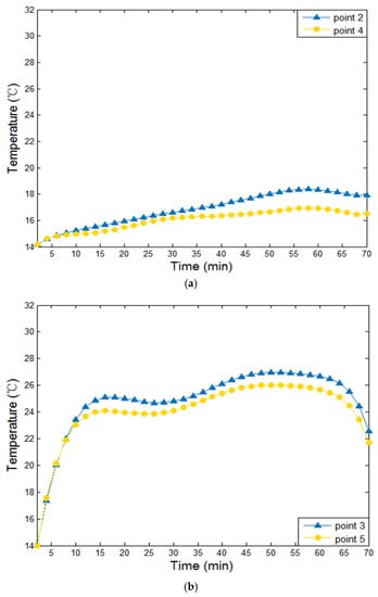
Figure 19. Temperature of the void boundary under lateral heating: (a) left side and (b) right side.

3. Conclusions

Experimental results showed that when the surface of the CFRTs was heated to approximately 26 °C, each measure point’s temperature on the surface was almost similar when the structure was in good condition. Once the void phenomenon appeared, temperature differences would occur in the void area.

For a single model, the temperature of the maximum void height was the highest, the temperature increase rate was the fastest, and the cooling rate was the slowest. The temperature of other measure points decreased with the decrease of the void height.

For the model with different void forms, the higher the void, the higher was the temperature. The average temperature difference of the measure points in the same position was above 1 °C. Because of the void’s existence, the heat absorbed by the upper surface transferred slowly into void area and then accumulated.

At the same time, there was a sudden temperature change on both sides of the interface. The temperature difference of the heating section was above 1.8 °C, and the temperature difference of the cooling section was above 1.2 °C, which were easy to identify. The more serious the void was, the wider was the gap between the void and the solid area. In addition, although the degree of temperature variation decreased after changing the heating direction, the temperature distribution could still be identified.

Numerical simulation showed that, due to the input of heat flux, the temperature difference of the concrete-filled steel tube structure between the void and the solid parts became greater, and the sudden temperature change of the interface also increased. The trend of this phenomenon was consistent with the experimental results. Moreover, the highest temperature point was also located in the largest void height. The temperature distribution of the whole model was uniform in the solid region and the temperature in the void region was higher than that in the solid region. There was an obvious and abrupt temperature change at the void interface.

In summary, the arch rib’s temperature was almost the same when the structure was good condition. However, when voids existed, the temperature difference of the surface was above 1 °C, and the temperature difference at the edge of the voids was even more serious. Therefore, the authors could evaluate the structure’s void. It is evident that the method used and based on a distributed temperature measurement is effective and feasible. This method has the advantages of low cost, the simple arrangement of sensors, and no need for a high-altitude operation. However, this method is suitable for the case of large voids in concrete-filled steel tubes, but not for the identification of voids.

In the future, researchers using this method would have to consider the natural environment’s influence and other factors, as well as the optimal placement of sensors to recognize the void interface of concrete-filled steel tubes and obtain a better qualitative and quantitative identification. Furthermore, the question of whether this method is suitable for concrete-filled steel tubular structures with surface coatings would also need further discussion.

References

- Chen, B.C.; Liu, F.Z.; Wei, J.G. Statistical analysis of 327 concrete filled steel tubular arch bridges. J. China Foreign Highw. 2011, 31, 96–103. [Google Scholar]
- Galietti, U.; Luprano, V.; Nenna, S.; Spagnolo, L.; Tundo, A. Non-destructive defect characterization of concrete structures reinforced by means of FRP. Infrared Phys. Technol. 2007, 49, 218–223. [Google Scholar] [CrossRef]
- Shams, M.; Saadeghvaziri, M.A. State of the art of concrete-filled steel tubular columns. ACI Struct. J. 1997, 94, 558–571. [Google Scholar]
- Chen, S.M.; Zhang, H.F. Numerical analysis of the axially loaded concrete filled steel tubecolumns with debonding separation at the steel-concrete interface. Steel Compos. Struct. 2012, 13, 277–293. [Google Scholar] [CrossRef]
- Fu, W.S.; Tian, H.S.; Sun, Z. Assessment of Deteriorations of Main Arch Ribs of CFST Arch Bridge Based on Inspection Results. Bridge Constr. 2013, 43, 47–51. [Google Scholar]
- Yang, J.; Han, X.; Yang, K.; Du, Y. Review on the research of void nondestructive testing technology for concrete filled steel tubular. J. China Foreign Highw. 2012, 5, 189–191. [Google Scholar]
- Lu, X.W.; Xu, R.; Wang, G.L. Common Defects in the Concrete-filled Steel Tube and Its Detection Methods. Constr. Technol. 2011, S1, 46–48. [Google Scholar]
- Pan, S.S.; Zhao, X.F.; Zhang, Z. Autoexcitation-based accelerometer array for interface separation detection of concrete-filled steel tubular arch bridge. Appl. Mech. Mater. 2014, 578–579, 995–999. [Google Scholar] [CrossRef]
- Khaira, A.; Srivastava, S.; Suhane, A. Analysis of relation between ultrasonic testing and microstructure: A step towards highly reliable fault detection. Eng. Rev. 2015, 35, 87–96. [Google Scholar]
- Petrovic, M.; Mihailovic, P.; Brajovic, L. Intensity fiber-optic sensor for structural health monitoring calibrated by impact tester. IEEE Sens. J. 2016, 16, 3047–3053. [Google Scholar] [CrossRef]
- Szymanik, B.; Chady, T.; Frankowski, P. Inspection of reinforcement concrete structures with active infrared thermography. AIP Conf. Proc. 2017, 1806. [Google Scholar] [CrossRef]
- Islam, M.A.; Kharkovsky, S. Detection and monitoring of gap in concrete-based composite structures using microwave dual waveguide sensor. IEEE Sens. J. 2017, 17, 986–993. [Google Scholar] [CrossRef]
- Fan, C.L.; Sun, F.R.; Yang, L. A quantitative identification technique for a two-dimensional subsurface defect based on surface temperature measurement. Heat Transf.-Asian Res. 2009, 38, 223–233. [Google Scholar] [CrossRef]
- Wang, J.T.; Huang, X.G.; Ding, M.Y.; Li, G.C. Wavelet analysis method of surface wave detection for steel tube concrete. Chin. J. Rock Mech. Eng. 2003, 11, 1878–1880. [Google Scholar]
- Pan, S.S.; Zhao, X.F.; Lv, X.J. Experiment on interface separation detection of concrete-filled steel tubular arch bridge using accelerometer array. Biotechnol. Indian J. 2013, 8, 1311–1317. [Google Scholar]
- Zhao, H.L.; Pan, S.S. Qualitative identification of interface separation of concrete-filled steel tube based on acceleration sensor. J. Shenyang Univ. 2014, 26, 230–233. [Google Scholar]
- Fu, B. Application Research on Quantitative Detection of Defect in Cfst Arch Bridge with Ultrasonic Detecting Technology. Master’s Thesis, Chongqing Jiaotong University, Chongqing, China, 2008. [Google Scholar]
- Mutlib, N.K.; Baharom, S.B.; El-Shafie, A.; Nuawi, Z.M. Ultrasonic health monitoring in structural engineering: buildings and bridges. Struct. Control Health Monit. 2016, 23, 409–422. [Google Scholar] [CrossRef]
- Ding, R.; Liu, H.W.; Luo, F.L.; Mu, T.M.; Hou, J. An investigation on optical fiber sensing of interface disengaging of steel tube confined concrete in arch bridges. J. Exp. Mech. 2004, 4, 493–499. [Google Scholar]
- Gifford, D.K.; Metrey, D.R.; Froggatt, M.E.; Rogers, M.E.; Sang, A.K. Monitoring strain during composite manufacturing using embedded distributed optical fiber sensing. In Proceedings of the International SAMPE Technical Conference, Aachen, Germany, 17–20 October 2011. [Google Scholar]
- Shang, Y.N. Application of infrared thermal diagnose technique in construction engineering detection. Shaanxi Archit. 2008, 156, 39–43. [Google Scholar]
- Chen, D.P.; Mao, H.X.; Xiao, Z.H. Infrared thermography NDT and its development. Comput. Meas. Control 2016, 24, 1–6. [Google Scholar]
- Gagnon, M.A.; Fortin, V.; Vallée, R.; Farley, V.; Lagueux, P.; Guyot, É.; Marcotte, F. Non-destructive testing of mid-IR optical fiber using infrared imaging. In Proceedings of the SPIE-The International Society for Optical Engineering, Baltimore, MA, USA, 18–21 April 2016. [Google Scholar]
- Cheng, C.C.; Cheng, T.M.; Chiang, C.H. Defect detection of concrete structures using both infrared thermography and elastic waves. Autom. Constr. 2008, 18, 87–92. [Google Scholar] [CrossRef]
- Khan, F.; Mohammad, B.; Antonios, K.; Ahmad, H.; Ivan, B. Modeling and experimental implementation of infrared thermography on concrete masonry structures. Infrared Phys. Technol. 2015, 69, 228–237. [Google Scholar] [CrossRef]
- Liu, Z.Y. Research on temperature field of cfst debonding members. China J. Highw. Transp. 2009, 22, 82–89. [Google Scholar]
- Chen, K.; Li, Y.D. Test and finite element calculation of solar temperature field of section of cfst arch rib. J. Highw. Transp. Res. Dev. 2012, 9, 77–84. [Google Scholar]
- Jeong, W.W.; Seong, J.H. Comparison of effects on technical variances of computational fluid dynamics (CFD) software based on finite element and finite volume methods. Int. J. Mech. Sci. 2014, 78, 19–26. [Google Scholar] [CrossRef]
- Tan, J.Y.; Zhao, J.M.; Liu, L.H. Meshless Method for Geometry Boundary Identification Problem of Heat Conduction. Numer. Heat Transf. B 2009, 55, 135–154. [Google Scholar] [CrossRef]
- Rus, G.; Gallego, R. Optimization algorithm for identification inverse problems with the boundary element method. Eng. Anal. Bound. Elem. 2002, 26, 315–327. [Google Scholar] [CrossRef]
© 2018 by the authors. Licensee MDPI, Basel, Switzerland. This article is an open access article distributed under the terms and conditions of the Creative Commons Attribution (CC BY) license (http://creativecommons.org/licenses/by/4.0/).