A Hybrid Fuzzy Analysis Network Process (FANP) and the Technique for Order of Preference by Similarity to Ideal Solution (TOPSIS) Approaches for Solid Waste to Energy Plant Location Selection in Vietnam

Abstract

Many research studies have applied the multi-criteria decision making (MCDM) approach to various fields of science and engineering, and this trend has been increasing for many years. One of the fields that the MCDM model has been employed is for location selection, yet very few studies consider this problem under fuzzy environmental conditions. In this research, the authors propose an MCDM approach, including fuzzy analysis network process (FANP), and the technique for order of preference by similarity to ideal solution (TOPSIS), for solid waste to energy plant location selection in Vietnam. In the first stage of this research, the ANP approach with fuzzy logic is applied to determine the weight of criteria. In the FANP model, the value of the criteria is provided by the experts so that the disadvantages of this model are that the input data, expressed in linguistic terms, depends on the experience of experts, and thus involves subjectivity. This is a reason why TOPSIS model was proposed for ranking alternatives in the final stage. Analysis shows that Hau Giang (Decision Making Unit 8 (DMU 8)) is the best location for building solid waste to energy plant, because it has the shortest geometric distance from the positive ideal solution (PIS) and the longest geometric distance from the negative ideal solution (NIS). The contribution of this research is a proposed hybrid FANP and TOPSIS approach for solid waste to energy plant location selection in Vietnam under fuzzy environmental conditions. This paper is also part of an evolution of a new hybrid model that is flexible and practical for decision makers. In addition, the research also provides a special, useful guideline in solid waste to energy plant location selection in many countries, as well as provides a guideline for location selection in other industries. Thus, this research makes significant contributions on both academic and practical fronts.

1. Introduction

Presently, the main energy resources in Vietnam are hydropower and thermal power. Vietnam’s fossil fuel resources have been exhausted due to overexploitation. Moreover, the plan to develop atomic energy has been halted. Vietnam has been importing materials and primary energy for electricity production, and the development of renewable energy will aid Vietnam to diversify and establish self-reliant power supply and environmental protection. Therefore, the government of Vietnam encourages the development of renewable energy, intelligent grid technology, and new energy technologies, as well as studies on how to exploit renewable energy sources. According to Vietnam’s Ministry of Natural Resources and Environment, the total domestic solid waste is approximately 12.8 million tons/year. In Vietnam, solid waste is mainly handled by landfilling and burning, which increases the cost of waste treatments and affects the environment. However, environmental pollution caused by waste incineration may raise concerns over the resident population coming down with the Not-In-My-Backyard (NIMBY) syndrome [1]. Therefore, the construction of solid waste to energy plant is needed in Vietnam.

The Resource Conservation and Recovery Act (RCRA) states that “solid waste” refers to any garbage or refuse, sludge from a wastewater treatment plant, water supply treatment plant, or air pollution control facility and other discarded material, resulting from industrial, commercial, mining, and agricultural operations, and from community activities. Nearly everything we do leaves behind some kind of waste. It is important to note that the definition of solid waste is not limited to waste that is physically solid. Many solid wastes are liquid, semi-solid, or contain gaseous material [2]. Hence, solid waste is one of the main causes of environmental pollution in developing countries [3,4,5]. There are many technologies for gaseous emission treatment [6,7].

A solid waste to energy plant is a waste management facility that combusts wastes to produce electricity. This type of power plant is sometimes referred to as a trash-to-energy, municipal waste incineration, energy recovery, or resource recovery plant [8]. The advantages of solid waste to energy is the use of closed process, energy production, reduction of greenhouse gases, and saving of land, and it being, essentially, a renewable energy [9].

Solid waste to energy technology is widely used in developing countries. The typical range of net electrical energy that can be produced is approximately 500–600 kWh per ton of waste incinerated.

Many research studies have applied the multi-criteria decision making (MCDM) approaches to various fields of science and engineering, a trend that has been increasing for many years. One of the fields that the MCDM model has been employed is in the location selection problem. Mahmoud A. Hassaan [10] proposed a geographic information systems (GIS) approach for siting a municipal solid waste incineration power plant in Egypt. Tavares et al. [11] used the analytical hierarchy process (AHP) and GIS for siting of an incineration plant for municipal solid waste. H. Y. Yap and J. D. Nixon [12] proposed a multi-criteria analysis of alternatives for energy recovery from municipal solid waste in India and the United Kingdom. Amy H. I. Lee et al. [13] presented a hybrid FAHP – Assurance Region (AR) – Data Envelopment Analysis (DEA) to assess the efficiencies of PV solar plant site candidates. Chia-Nan Wang et al. [14] proposed a hybrid model including DEA–FAHP–TOPSIS for solar power plant location selection in Vietnam. P. Aragonés-Beltrán et al. [15] used ANP for selection of photovoltaic (PV) solar power plant investment projects.

Ali et al. [16] proposed a hybrid GIS and MCDM approach to define the best place for wind farm location. Suh and Brownson [17] proposed GIS and AHP approaches to select PV solar plant sites. Noorollahi et al. [18] combined GIS and fuzzy AHP for land analyses in solar farm site. Audrius Čereška et al. [19] used MCDM for analyzing of steel wire rope diagnostic data.

A generic process of MCDM is shown in Figure 1.

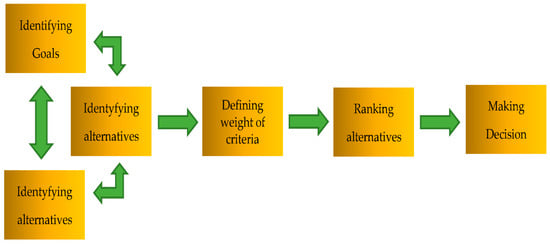
Figure 1. A generic process of multi-criteria decision making (MCDM).

Decision makers should follow a four-stage procedure when making location selection. These steps are as follows and as shown in Figure 2 [20,21].

Figure 2. General methodology of location selection problem.

Step 1: Identify location attributes. In this stage, all attributes that affect the organization will be considered.

Step 2: Identify alternatives. Once decision makers know what attributes affect the organization, they can define alternatives that satisfy the selected attributes.

Step 3: Evaluate alternatives. After a set of alternatives are built, all potential alternatives will be evaluated and ranked by quantitative or qualitative methods.

Step 4: Make a decision. The best alternative will be defined base on the highest-ranking score in the final step.

Gan et al. [22] used integrated Triangular Fuzzy Numbers (TFN)-AHP-DEA approaches for renewable energy projects analyzed economic feasibility. Liu et al. [23] proposed a hybrid MCDM model by combining data envelopment analysis (DEA) and the Malmquist model for evaluating the total factor energy efficiency. Asad Asadzadel et al. [24] proposed TOPSIS model for assessing site selection of new towns. Maria Rashidi et al. [25] presented the developed decision support system for asset management of steel bridges within acceptable limits of safety, functionality, and sustainability by using AHP model.

This research proposes a MCDM model including FANP and TOPSIS for solid waste to energy plant location selection in Vietnam under uncertain environmental conditions. In the first stage of this research, FANP is applied to determine the weight of criteria. The steps for implementing the FANP model are as follows:

Step 1: Building FANP model.

Step 2: Set up pair comparison matrix.

Step 3: Calculate maximum individual value.

Step 4: Check consistency. Calculate the vector of the matrix.

Step 5: Form the super matrix.

In the FANP, AHP, or FAHP model, the value of the criteria is provided by the experts, so the disadvantage of the model is that the input data, expressed in linguistic terms, depends on the experience of experts, and thus involves subjectivity. This is a reason why the TOPSIS model is proposed for ranking alternatives in the final stage. The TOPSIS model was employed to rank potential sites. Optimal options have the shortest geometric distance from the positive ideal solution (PIS) and the longest geometric distance from the negative ideal solution (NIS). The advantage of this method is its simplicity and ability to yield an indisputable preference order [26,27]. There are six steps in TOPSIS process, as follows:

Step 1: Determining the normalized decision matrix.

Step 2: Calculating the weight normalized value.

Step 3: Calculating the PIS ($D^{+}$) and PIS ($D^{-}$).

Step 4: Determining a distance of the PIS $\left(Q_x^{+}\right).$

Step 5: Determining the relationship proximal.

Step 6: Determining the best option with the maximum value of $C_a$.

The remainder of the article provides background materials to assist in developing the MCDM model. Then, a hybrid FANP–TOPSIS approach is presented to select the best location for building of a solid waste to energy plant from among eight potential locations in Vietnam. The results, discussion, and the contributions are presented at the end of the paper.

2. Material and Methodology

2.1. Research Development

In this research, we present a hybrid fuzzy ANP and TOPSIS approaches to select the best site for building a solid waste to energy plant in Vietnam. There are three steps in this study, as shown in Figure 3:

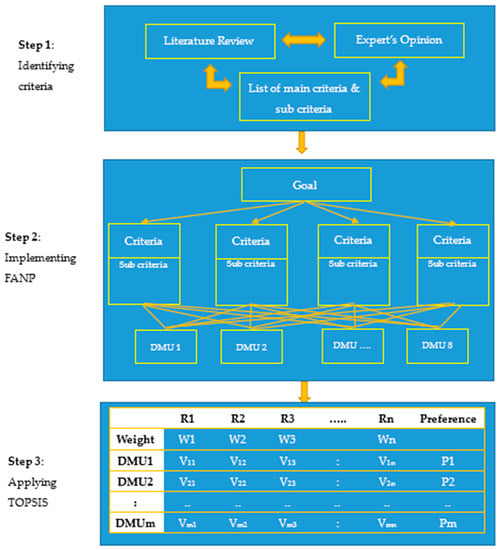
Figure 3. Research methodologies.

Step 1: Identify criteria. In this stage, the criteria for selecting the best location for building solid waste to energy plant will be defined by expert’s interviews and literature review from others’ research. All of the attributes are shown in Figure 3.

Step 2: Implement fuzzy analysis network process model (FANP). The FANP model is the most effective tool for defining the weight of the criteria. The weight of criteria will be calculated based on economic factors, technical requirements factors, environment factors, and social factors. The weight of all criteria will be used in TOPSIS model.

Step 3: Apply the technique for order of preference by similarity to the ideal solution (TOPSIS) model. The TOPSIS approach is used to rank potential locations. The optimal alternatives will have the shortest geometric distance from the positive ideal solution (PIS) and the longest geometric distance from the negative ideal solution (NIS).

2.2. Methodology

2.2.1. Fuzzy Analytic Network Process (FANP)

(1) Analytic Network Process (ANP)

The ANP model was developed to overcome the limitations of AHP, taking into account the hierarchy and interactions between the selection criteria. Moreover, the dynamics and complexity of the majority of decision making environments make ANP an effective tool in addressing such situations. According to Sarkis, ANP is a powerful decision making technique for analyzing key issues related to green supply chain management and environmental business operations, but both AHP and ANP require a resolution. Strategic planning ANP is a combination of two parts [28,29]:

-

Primary and secondary criteria that control the interactions.

-

The grid effect of elements and clusters.

The goal of the ANP is to use qualitative methods to rank qualitative decisions and to select one or more alternatives that meet the criteria.

(2) Fuzzy Analytic Network Process

Zadeh (1965) [30] introduced the theory to deal with uncertainty due to imprecision and vagueness. There are many forms of fuzzy numbers, such as trapezoidal fuzzy numbers, triangular fuzzy numbers, etc. However triangular fuzzy numbers are often used by efficiency and ease of use. In this study, vendor evaluations were made based on triangular fuzzy numbers, so this fuzzy number was studied [31,32,33,34,35]. The fuzzy triangular numbers are shown in Figure 4.

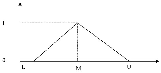
Figure 4. Fuzzy triangular number.

$$\mu \left(x\right)=\{\begin{array}{c}\frac{x -L}{M -L}, L\le x\le M\\ \frac{U -x}{U -M}, M\le x\le U\\ 0, otherwise\end{array}$$

(1)

If L = M = U, the fuzzy number A becomes real number. Thus, real numbers are special cases of fuzzy numbers [36].

Fuzzy set theory is a perfect means for modeling uncertainty (or imprecision) arising from mental phenomena, which are neither random nor stochastic. This attitude towards the uncertainty of human behavior led to the study of a relatively new decision analysis field: fuzzy analytical network process [37].

The procedure for implementing the FANP method is as follows:

Step 1: Building FANP model.

Construction of the FANP model structure. Set the hierarchy and define the relationship between the criteria as well as the supplier.

Step 2: Set up pair comparison matrix.

A pairwise comparison of fuzzy numbers is used to perform a pairwise comparison between criteria. The pair comparison matrix is presented as follows:

$$\widetilde{A^k}=\left[\begin{array}{ccc}\widetilde{a_{11}^k}& \widetilde{a_{12}^k}& \cdots \\ \begin{array}{c}\widetilde{a_{21}^k}\\ \cdots \end{array}& \begin{array}{c}\widetilde{a_{22}^k}\\ \cdots \end{array}& \begin{array}{c}\cdots \\ \cdots \end{array}\\ \widetilde{a_{n1}^k}& \widetilde{a_{n2}^k}& \cdots \end{array} \begin{array}{c}\widetilde{a_{1n}^k}\\ \widetilde{a_{2n}^k}\\ \begin{array}{c}\cdots \\ \widetilde{a_{nn}^k}\end{array}\end{array}\right],$$

(2)

where

$\widetilde{A^k}$ is called a pairwise comparative matrix of fuzzy elements,

$\widetilde{a_{nn}^{k }}$ is the triangular fuzzy mean value when comparing the pair of priorities between the elements.

Converting fuzzy numbers to real numbers, triangular fuzzy trigonometric methods are presented as follows [38]:

$$\begin{gathered} t_{\alpha ,\beta }\left({\overline{\alpha }}_{ij}\right)=\left[\beta f_{\alpha }\right(L_{ij})+(1-\beta \left)f_{\alpha }\right(U_{ij}\left)\right]; \\ 0\le \beta \le 1,0\le \alpha \le 1 \end{gathered}$$

(3)

where

$$f_{\alpha }\left(L_{ij}\right)=(M_{ij}-L_{ij})\alpha +L_{ij}$$

(4)

$$f_{\alpha }\left(U_{ij}\right)=U_{ij}-(U_{ij}-M_{ij})\alpha .$$

(5)

When matching the diagonal matrix, we have

$$\begin{gathered} t_{\alpha ,\beta }({\overline{\alpha }}_{ij})=\frac{1}{t_{\alpha ,\beta }\left({\overline{\alpha }}_{ij}\right)} \\ 0\le \beta \le 1,0\le \alpha \le 1, i>j. \end{gathered}$$

(6)

After comparing the fuzzy pairwise comparison matrix, we obtain a matrix that compares the real numbers. This comparison is made between pairs of indicators and is combined into a matrix of n lines and n columns (n: is the number of indicators). Element shows the importance of the indicator i versus the column criteria.

$$A={\left(m_{ij}\right)}_{n\times n}=\left[\begin{array}{cc}\begin{array}{cc}1& m_{12}\\ m_{21}& 1\end{array}& \begin{array}{cc}\dots & m_{1n}\\ \dots & m_{2n}\end{array}\\ \begin{array}{cc}⋮& ⋮\\ m_{n1}& m_{n2}\end{array}& \begin{array}{cc}⋮& ⋮\\ \dots & 1\end{array}\end{array}\right]$$

(7)

To evaluate the priority in the FANP model, we use the scale presented in the Table 1 as follows.

Table 1. Fuzzy conversion scale [39].

Intensity of Fuzzy Scale	Linguistic Variables for Relative Weights of Criteria
$\tilde{1}=\left(1,1,1\right)$	Equally important
$\tilde{3}=\left(2,3,4\right)$	Moderately important
$\tilde{5}=\left(4,5,6\right)$	Strongly important
$\tilde{7}=\left(7,8,9\right)$	Very strongly important
$\tilde{9}=\left(9,9,9\right)$	Extremely strongly important
$\tilde{2},\tilde{4}\widetilde{,6},\tilde{8}$	Intermediate values between two adjacent judgments; $\tilde{2}=\left(1,2,3\right)$; $\tilde{4}=\left(3,4,5\right)$; $\tilde{6}=\left(5,6,7\right)$; $\tilde{8}=\left(7,8,9\right)$;

After the fuzzy decomposition, in the form of the real comparison matrix. The scale that was suggested by Saaty for AHP and ANP can be used. These scales are shown in Table 2 [40].

Table 2. Priority rating scale.

Priority Level	Number
Equally preferred	1
Moderately preferred	3
Strongly preferred	5
Very strongly preferred	7
Extremely preferred	9
Intermediate judgment values	2, 4, 6, 8

Step 3: Calculate maximum individual value.

To calculate the maximum specific value for the indicator. In particular, the most widely used is lambda max (max) by Saaty’s proposition [40]:

$$\left|A-{\lambda }_{\max }.I\right|=0,$$

(8)

where

• ${\lambda }_{\max }$: the maximum value of the matrix.
• A: Comparative matrix of pairs of elements.
• I: unit matrix of the same level with matrix A.

Step 4: Check consistency. Calculate the vector of the matrix.

After calculating maximum individual value, Saaty [40] can use the consistency ratio (CR). This ratio compares the degree of consistency with the (random) objectivity of the data:

$$CR=\frac{CI}{RI},$$

(9)

where

• CI: consistency index,
• RI: random index.

If CR $\le 0.1$ is satisfactory, otherwise if CR $\ge$ 0.1 then we must conduct a reevaluation of the pair comparison matrix.

$$CI=\frac{{\lambda }_{\max }-n}{n-1},$$

(10)

where

• ${\lambda }_{\max }$ is the maximum value of the matrix,
• n is the number of indicators.

For each n-level comparison matrix, Saaty [40] tested the creation of random matrices and calculated the RI (random index) corresponding to the number of indicators as shown in the Table 3.

Table 3. Randomized index values corresponding to indicators.

N	1	2	3	4	5	6	7	8	9	10
R	0	0	0.52	0.90	1.12	1.24	1.32	1.41	1.45	1.49

Step 5: Form the super matrix

After completing the above steps, a super matrix is formed in Table 4 as follows:

Table 4. Super matrix.

0	U12	0
U21	U22	U23
0	0	0

where

-

U₁₂ is a matrix formed from the matrix’s own vector when comparing the choices for each criterion.

-

U₂₁ is a matrix formed from its own vector when comparing the criteria for each choice.

-

U₂₂ is a matrix formed from its own vector when comparing the interaction effect between the criteria.

-

U₂₃ is a matrix formed from the matrix’s own vector when comparing the criteria with each other.

2.2.2. TOPSIS Model

TOPSIS model was proposed Hwang and Yoon [41]. The main concept of TOPSIS is that the best options should have the shortest geometric distance from the positive ideal solution (PIS) and the longest geometric distance from the negative ideal solution (NIS) [42]. There are m alternatives and n criteria, and the result of TOPSIS model shows the score of each option [43]. There are six steps of TOPSIS process, as below:

Step 1: Determining the normalized decision matrix, raw values (a_ij) are transferred to normalized values (n_ij) by

$$k_{xy}=\frac{b_{xy}}{\sqrt{{{\displaystyle \sum }}_x^e{b}_{xy}^2}}, x=1,\dots ,e;y=1,\dots ,k.$$

(11)

Step 2: Calculating the weight normalized value (v_ij), by

$$f_{xy}=P_{xy}{h}_{xy}, x=1,\dots .,e;y=1,\dots ,k.$$

(12)

where Pj is the weight of the $x^{tk}$ criterion and ${{\displaystyle \sum }}_{y=1}^k{p}_p=1$.

Step 3: Calculating the PIS ($D^{+}$) and PIS ($D^{-}$), where $l_x^{+}$ indicate the maximum values of $f_{xy}$ and $f_x^{-}$ indicates the minimum value $f_{xy}$:

$$D^{+}=\left\{f_1^{+},\dots ,f_h^{+}\right\}=\left\{\left(\underset{y}{\max }{f}_{xy}|x\in A\right),\left(\underset{y}{\min }{f}_{xy}|x\in A\right)\right\},$$

(13)

$$D^{-}=\left\{f_1^{-},\dots ,f_n^{-}\right\}=\left\{\left(\underset{y}{\min }{f}_{xy}|x\in A\right),\left(\underset{y}{\max }{f}_{xy}|y\in B\right)\right\},$$

(14)

Step 4: Determining a distance of the PIS $\left(Q_x^{+}\right)$ separately by

$$Q_x^{+}={\left\{{\displaystyle \sum }_{y=1}^k{\left(f_{xy}-f_y^{+}\right)}^2\right\}}^{\frac{1}{2}}, x=1, \dots , e$$

(15)

Similarly, the separation from the NIS $\left(Q_i^{-}\right)$ is given as

$$Q_x^{-}={\left\{{{\displaystyle \sum }}_{y=1}^k{\left(f_{xy}-f_y^{-}\right)}^2\right\}}^{\frac{1}{2}}, x=1, \dots , e.$$

(16)

Step 5: Determining the relationship proximal to the problem-solving model:

$$C_x=\frac{Q_x^{-}}{Q_x^{+}+Q_x^{-}}, x=1,\dots ,e.$$

(17)

Step 6: Determining the best option with the maximum value of $C_a$.

3. Case Study

The impact of the industrialization and modernization has resulted in ever-increasing solid waste. Vietnam is among five countries in the world with the most solid waste discarded into the ocean. Solid waste in Vietnam includes garbage, construction debris, commercial refuse, hospital waste, etc. A summary of solid waste in Vietnam is shown in Figure 5.

Figure 5. Solid waste in Vietnam.

In this research, the authors analyzed eight potential locations for a solid waste to energy plant in Vietnam. The information about eight potential locations is shown in Table 5.

Table 5. Potential locations for building a solid waste to energy plant.

No	Potential Location	Decision Making Unit (DMU)
1	Long An	DMU 1
2	Tien Giang	DMU 2
3	Can Tho	DMU 3
4	Ben Tre	DMU 4
5	An Giang	DMU 5
6	Vinh Long	DMU 6
7	Dong Thap	DMU 7
8	Hau Giang	DMU 8

The geographical location of eight of potential locations (DMU) are shown in Figure 6.

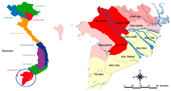
Figure 6. The geographical location of DMU. (Source: UN Development Programme.)

Based on the results of Expert’s interviews and literature review, the hierarchical structures of the FANP was contracture, as shown in Figure 7.

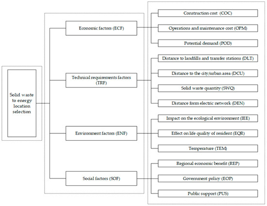
Figure 7. The hierarchical structures of the fuzzy analysis network process (FANP).

A fuzzy comparison matrix for all criteria from FANP model is shown in Table 6.

Table 6. Fuzzy comparison matrices for criteria.

Criteria	EFC	ENF	SOF	TRF
ECF	(1,1,1)	(2,3,4)	(1,2,3)	(3,4,5)
ENF	(1/4,1/3,1/2)	(1,1,1)	(1/4,1/3,1/2)	(1,1,1)
SOF	(1/3,1/2,1)	(2,3,4)	(1,1,1)	(4,5,6)
TRF	(1/5,1/4,1/3)	(1,1,1)	(1/6,1/5,1/4)	(1,1,1)

We used the triangular fuzzy number to convert the fuzzy numbers to real numbers. During the defuzzification, the authors obtain the coefficients α = 0.5 and β = 0.5.

$${\mathrm{g}}_{0.5,0.5}\left(\overline{a_{ECF,ENF}}\right)=\left[\right(0.5\times 2.5)+(1-0.5)\times 3.5]=3$$

f_0.5(L_EFC,ENF) = (3 − 2) × 0.5 + 2 = 2.5

f_0.5(U_EFC,ENF) = 4 − (4 − 3) × 0.5 = 3.5

$${\mathrm{g}}_{0.5,0.5}\left(\overline{a_{ENF,EFC}}\right)=1/3$$

The remaining calculations are similar to the above calculation, as well as the fuzzy number priority point. The real number priority when comparing the main criteria pairs is presented in Table 7.

Table 7. Real number priority.

Criteria	ECF	ENF	SOF	TRF
ECF	1	3	2	4
ENF	1/3	1	1/3	1
SOF	1/2	3	1	5
TRF	1/4	1	1/5	1

To calculate the maximum individual value as follows:

AM1 = (1 × 3 × 2 × 4)^1/4 = 2.21

AM2 = (1/3 × 1 × 1/3 × 1)^1/4 = 0.58

AM3 = (1/2 × 3 × 1 × 5)^1/4 = 1.64

AM4 = (1/4 × 1 × 1/5 × 1)^1/4 = 0.47

$$\sum \mathrm{AM}=\mathrm{AM}1+\mathrm{AM}2+\mathrm{AM}3+\mathrm{AM}4+\mathrm{AM}5=4.9$$

$${\omega }_1=\frac{2.21}{4.9}=0.45$$

$${\omega }_2=\frac{0.58}{4.9}=0.12$$

$${\omega }_3=\frac{1.64}{4.9}=0.33$$

$${\omega }_4=\frac{0.47}{4.9}=0.1$$

$$\left[\begin{array}{cccc}1& 3& 2& 4\\ 1/3& 1& 1/3& 1\\ 1/2& 3& 1& 5\\ 1/4& 1& 1/5& 1\end{array}\right]\times \left[\begin{array}{c}0.45\\ 0.12\\ 0.33\\ 0.1\end{array}\right]=\left[\begin{array}{c}1.87\\ 0.48\\ 1.42\\ 0.4\end{array}\right]$$

$$\left[\begin{array}{c}1.87\\ 0.48\\ 1.42\\ 0.4\end{array}\right]/\left[\begin{array}{c}0.45\\ 0.12\\ 0.33\\ 0.1\end{array}\right]=\left[\begin{array}{c}4.16\\ 4\\ 4.30\\ 4\end{array}\right]$$

With the number of criteria is 4, we get n = 4, λ_max and CI are calculated as follows:

$${\lambda }_{\max }=\frac{4.16+4+4.30+4}{4}=4.12$$

$$CI=\frac{{\lambda }_{\max }-n}{n-1}=\frac{4.12-4}{4-1}=0.04$$

For CR, with n = 4 we get RI = 0.9.

$$CR=\frac{CI}{RI}=\frac{0.04}{0.9}=0.044$$

We have CR = 0.09598 ≤ 0.1, so the pairwise comparison data is consistent and need not to be re-evaluated. The results of the pair comparison between the main criteria are presented in Table 8.

Table 8. Fuzzy comparison matrices for criteria.

Criteria	ECF	ENF	SOF	TRF	Weight
ECF	(1,1,1)	(2,3,4)	(1,2,3)	(3,4,5)	0.45
ENF	(1/4,1/3,1/2)	(1,1,1)	(1/4,1/3,1/2)	(1,1,1)	0.12
SOF	(1/3,1/2,1)	(2,3,4)	(1,1,1)	(4,5,6)	0.33
TRF	(1/5,1/4,1/3)	(1,1,1)	(1/6,1/5,1/4)	(1,1,1)	0.1
Total					1
CR = 0.044

All the remaining calculation are shown in Appendix A.

The weight of all subcriteria calculated in FANP model are shown in Table 9.

Table 9. The weight of 13 subcriteria.

No	Subcriteria	Weight
1	COC	0.09995
2	DCU	0.07521
3	DEN	0.0473
4	DLT	0.03181
5	EOP	0.03948
6	EQR	0.15249
7	IEE	0.16369
8	OPM	0.10082
9	POD	0.10397
10	PUS	0.03423
11	REP	0.04143
12	SWQ	0.06067
13	TEM	0.04896

TOPSIS model is then applied for ranking all the potential locations. The normalized weight matrix (TOPSIS) are shown in Table 10.

Table 10. Normalized weight matrix (TOPSIS).

Subcriteria	DMUs
	DMU 1	DMU 2	DMU 3	DMU 4	DMU 5	DMU 6	DMU 7	DMU 8
COC	0.0260	0.0390	0.0520	0.0260	0.0390	0.0260	0.0390	0.0260
OPM	0.0472	0.0236	0.0236	0.0472	0.0472	0.0354	0.0236	0.0236
POD	0.0466	0.0362	0.0310	0.0414	0.0259	0.0414	0.0310	0.0362
DLT	0.0106	0.0106	0.0106	0.0106	0.0141	0.0071	0.0106	0.0141
DCU	0.0272	0.0272	0.0272	0.0272	0.0272	0.0362	0.0181	0.0181
SWQ	0.0182	0.0243	0.0213	0.0243	0.0243	0.0182	0.0213	0.0182
DEN	0.0168	0.0168	0.0112	0.0225	0.0112	0.0225	0.0112	0.0168
IEE	0.0452	0.0226	0.0339	0.0565	0.0565	0.0565	0.0565	0.1017
EQR	0.0490	0.0490	0.0490	0.0588	0.0294	0.0392	0.0490	0.0882
TEM	0.0183	0.0138	0.0183	0.0160	0.0206	0.0160	0.0160	0.0183
REP	0.0174	0.0116	0.0135	0.0155	0.0155	0.0135	0.0174	0.0116
EOP	0.0168	0.0168	0.0131	0.0150	0.0112	0.0131	0.0131	0.0112
PUS	0.0124	0.0124	0.0108	0.0093	0.0139	0.0139	0.0124	0.0108

4. Results and Discussion

Solid waste to energy plant location selection has been identified as an important problem which could affect to the economic and social characteristics of a society. It can be seen that location selection is complicated, in that decision makers must have broad perspectives concerning qualitative and quantitative factors.

As an empirical study, the authors collect data from 8 potential locations in Vietnam. A hierarchical structure to select the best place was built with four main criteria (including 13 subcriteria). Completion of a questionnaire for analyzing in FANP model were done by expert opinion and literature reviews from other research. The ANP model was combined with fuzzy logic to define a priority of each potential location. Then, the TOPSIS model is used for ranking location.

In Figure 8, Hau Giang (DMU 8) has the shortest geometric distance from the PIS and the longest geometric distance from the NIS.

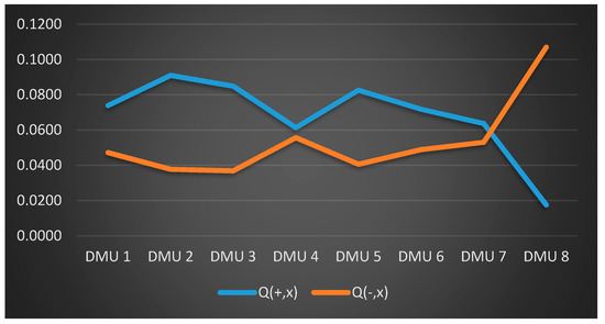
Figure 8. Geometric distance from positive ideal solution (PIS) and negative ideal solution (NIS).

The results of TOPSIS model are shown in Figure 9; based on the final performance score C_x, the final locations ranking list are DMU 8, DMU 4, DMU 7, DMU 6, DMU 1, DMU 5, DMU 3, and DMU 2. The results show that DMU 8 (Hau Giang) is the best location for building a solid waste to energy plant in Vietnam.

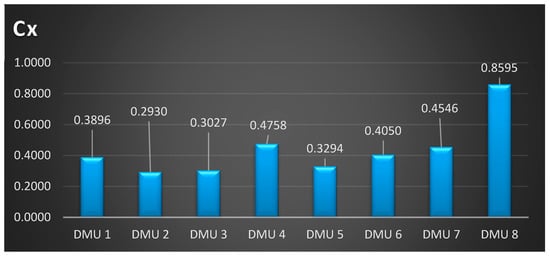
Figure 9. Final performance in technique for order of preference by similarity to ideal solution (TOPSIS) model.

5. Conclusions

Renewable energy plant location selection requires involvement of different decision makers who must evaluate both qualitative and quantitative factors. The fact that economic factors, technical requirements factors, environment factors, and social factors for solid waste to energy plant location selection are considered makes the process more complex. Many studies have applied the MCDM approach to various fields of science and engineering, and this trend has been increasing for many years. One of the fields that the MCDM model has been employed is for location selection, yet very few studies consider this problem under fuzzy environmental conditions. Besides, there is no research that applies the MCDM model for solid waste to energy plant location selection in Vietnam. This is a reason why we proposed a hybrid fuzzy analysis network process (FANP) and the technique for order of preference by similarity to ideal solution (TOPSIS) for solid waste to energy plant location selection in Vietnam.

In the first stage of this research, FANP is applied to determine the weight of criteria. In the FANP model, the value of the criteria is given by the experts, so the disadvantage is that the input data, expressed in linguistic terms, depends on the experience of experts, and is thus subjective. This is a reason why the TOPSIS model was proposed for ranking alternatives in the final stage. The best place for building solid waste to energy plant was concluded to be Hau Giang (DMU 8), because it has the shortest geometric distance from the positive ideal solution (PIS) and the longest geometric distance from the negative ideal solution (NIS).

The contribution of this research is a proposed hybrid FANP and TOPSIS for renewable energy plant location selection in Vietnam under fuzzy environment conditions. Building solid waste to energy plant brings many economic and environmental benefits. Building solid waste to energy plant also creates a new source of renewable energy. This paper also part of the evolution of a new approach that is flexible and practicable to the decision maker. This research provides a useful guideline for solid waste to energy plant location selection in many countries, as well as a guideline for location selection in other industries. Thus, this research has great contributions on academic and practical fronts.

In future research, this hybrid model can be employed to many different countries. In addition, different methods, such as data envelopment analysis (DEA) or the preference ranking organization method for enrichment of evaluations (PROMETHEE), etc., could also be combined for evaluating and selecting locations.

References

- Hou, H.; Li, S.; Lu, Q. Gaseous emission of monocombustion of sewage sludge in a circulating fluidized bed. Ind. Eng. Chem. Res. 2013, 52, 5556–5562. [Google Scholar] [CrossRef]
- United States Environmental Protection Agency. Criteria for the Definition of Solid Waste and Solid and Hazardous Waste Exclusions; EPA: Washington, DC, USA, 2018.
- Costi, P.; Minciardi, R.; Robba, M.; Rovatti, M.; Sacile, R. An environmentally sustainable decision model for urban solid waste management. Waste Manag. 2004, 24, 277–295. [Google Scholar] [CrossRef]
- Fiorucci, P.; Minciardi, R.; Robba, M.; Sacile, R. Solid waste management in urban areas: Development and application of a decision support system. Resour. Conserv. Recycl. 2003, 37, 301–328. [Google Scholar] [CrossRef]
- Nakhla, D.A.; Hassan, M.G.; Haggar, S.E. Impact of biomass in egypt on climate change. Nat. Sci. 2013, 5, 678–684. [Google Scholar] [CrossRef]
- Cheung, W.H.; Lee, V.K.C.; McKay, G. Minimizing dioxin emissions from integrated msw thermal treatment. Environ. Sci. Technol. 2007, 41, 2001–2007. [Google Scholar] [CrossRef] [PubMed]
- Lancia, A.; Karatza, D.; Musmarra, D.; Pepe, F. Adsorption of mercuric chloride from simulated incinerator exhaust gas by means of sorbalittm particles. J. Chem. Eng. Jpn. 1996, 29, 939–946. [Google Scholar] [CrossRef]
- Weinstein, P.E. Waste-to-Energy as a Key Component of Integrated Solid Waste Management for Santiago, Chile: A Cost-Benefit Analysis; Fu Foundation School of Engineering and Applied Science, Columbia University: New York, NY, USA, 2006. [Google Scholar]
- Psomopoulos, C.; Bourka, A.; Themelis, N.J. Waste-to-energy: A review of the status and benefits in USA. Waste Manag. 2009, 29, 1718–1724. [Google Scholar] [CrossRef] [PubMed]
- Hassaan, M.A. A gis-based suitability analysis for siting a solid waste incineration power plant in an urban area case study: Alexandria governorate, Egypt. J. Geogr. Inform. Syst. 2015, 7, 643–657. [Google Scholar] [CrossRef]
- Tavares, G.; Zsigraiová, Z.; Semiao, V. Multi-criteria gis-based siting of an incineration plant for municipal solid waste. Waste Manag. 2011, 31, 1960–1972. [Google Scholar] [CrossRef] [PubMed]
- Yap, H.Y.; Nixon, J.D. A multi-criteria analysis of options for energy recovery from municipal solid waste in India and the UK. Waste Manag. 2015, 46, 265–277. [Google Scholar] [CrossRef] [PubMed]
- Lee, A.H.I.; Kang, H.-Y.; Lin, C.-Y.; Shen, K.-C. An integrated decision-making model for the location of a pv solar plant. Sustainability 2015, 7, 13522–13541. [Google Scholar] [CrossRef]
- Wang, C.-N.; Nguyen, V.T.; Thai, H.T.N.; Duong, D.H. Multi-criteria decision making (MCDM) approaches for solar power plant location selection in viet nam. Energies 2018, 11, 1504. [Google Scholar] [CrossRef]
- Aragonés-Beltrán, P.; Chaparro-González, F.; Ferrando, J.P.P.; García-Melón, M. Selection of photovoltaic solar power plant investment projects-an anp approach. Int. J. Environ. Chem. Ecol. Geol. Geophys. Eng. 2008, 128–136. [Google Scholar] [CrossRef]
- Ali, S.; Lee, S.-M.; Jang, C.-M. Determination of the most optimal on-shore wind farm site location using a GIS-MCDM methodology: Evaluating the case of south korea. Energies 2017, 10, 2072. [Google Scholar] [CrossRef]
- Suh, J.; Brownson, J.R.S. Solar farm suitability using geographic information system fuzzy sets and analytic hierarchy processes: Case study of ulleung island, Korea. Energies 2016, 9, 648. [Google Scholar] [CrossRef]
- Noorollahi, E.; Fadai, D.; Shirazi, M.A.; Ghodsipour, S.H. Land suitability analysis for solar farms exploitation using gis and fuzzy analytic hierarchy process (FAHP)—A case study of Iran. Energies 2016, 9, 643. [Google Scholar] [CrossRef]
- ˇCereška, A.; Zavadskas, E.K.; Bucinskas, V.; Podvezko, V.; Sutinys, E. Analysis of steel wire rope diagnostic data applying multi-criteria methods. Appl. Sci. 2018, 8, 260. [Google Scholar] [CrossRef]
- Reid, R.D.; Sanders, N.R. Operations Management; Wiley: Hoboken, NJ, USA, 2009. [Google Scholar]
- Belton, V.; Stewart, T. Multiple Criteria Decision Analysis: An Integrated Approach; Kluwer Academic: Boston, MA, USA, 2002. [Google Scholar]
- Gan, L.; Xu, D.; Hu, L.; Wang, L. Economic feasibility analysis for renewable energy project using an integrated TFN–AHP–DEA approach on the basis of consumer utility. Energies 2017, 10, 2089. [Google Scholar] [CrossRef]
- Liu, J.-P.; Yang, Q.-R.; He, L. Total-factor energy efficiency (TFEE) evaluation on thermal power industry with DEA, malmquist and multiple regression techniques. Energies 2017, 10, 1039. [Google Scholar] [CrossRef]
- Asadzadeh, A.; Sikder, S.K.; Mahmoudi, F.; Kötter, T. Assessing site selection of new towns using topsis method under entropy logic: A case study: New towns of tehran metropolitan region (TMR). Environ. Manag. Sustain. Dev. 2014, 3, 123–137. [Google Scholar] [CrossRef]
- Rashidi, M.; Ghodrat, M.; Samali, B.; Kendall, B.; Zhang, C. Remedial modelling of steel bridges through application of analytical hierarchy process (AHP). Appl. Sci. 2017, 7, 168. [Google Scholar] [CrossRef]
- Feng, C.-M.; Wang, R.-T. Performance evaluation for airlines including the consideration of financial ratios. J. Air. Transp. Manag. 2000, 6, 133–142. [Google Scholar] [CrossRef]
- Sen, P.; Yang, J.-B. Multiple Criteria Decision Support in Engineering Design; Springer: London, UK, 1998. [Google Scholar]
- Sarkis, J. A strategic decision framework for green supply chain management. J. Clean. Prod. 2003, 11, 397–409. [Google Scholar] [CrossRef]
- Saaty, T.L. Decision Making with Dependence and Feedback: The Analytic Network Process; Rws Publications: Pittsburgh, PA, USA, 1996. [Google Scholar]
- Zadeh, L.A. Fuzzy sets. Inform. Control. 1965, 8, 338–353. [Google Scholar] [CrossRef]
- Lee, A.H.I. A fuzzy supplier selection model with the consideration of benefits, opportunities, costs and risks. Expert. Syst. Appl. 2009, 36, 2879–2893. [Google Scholar] [CrossRef]
- Lee, A.H.I.; Kang, H.-Y.; Hsu, C.-F.; Hung, H.-C. A green supplier selection model for high-tech industry. Expert. Syst. Appl. 2009, 36, 7917–7927. [Google Scholar] [CrossRef]
- Lee, A.H.I.; Kang, H.-Y.; Chang, C.-T. Fuzzy multiple goal programming applied to tft-lcd supplier selection by downstream manufacturers. Expert. Syst. Appl. 2009, 36, 6318–6325. [Google Scholar] [CrossRef]
- Lee, A.H.I.; Kang, H.-Y.; Wang, W.-P. Analysis of priority mix planning for the fabrication of semiconductors under uncertainty. Int. J. Adv. Manuf. Technol. 2006, 28, 351–361. [Google Scholar] [CrossRef]
- Cheng, C.-H. Evaluating weapon systems using ranking fuzzy numbers. Fuzzy Sets Syst. 1999, 107, 25–35. [Google Scholar] [CrossRef]
- Dehghani, M.; Esmaeilian, M.; Tavakkoli-Moghaddam, R. Employing fuzzy anp for green supplier selection and order allocations: A case study. Int. J. Econ. Manag. Soc. Sci. 2013, 2, 565–575. [Google Scholar]
- Kahraman, C.; Ertay, T.; Büyüközkan, G. A fuzzy optimization model for QFD planning process using analytic network approach. Eur. J. Oper. Res. 2006, 171, 390–411. [Google Scholar] [CrossRef]
- Lin, R.; Lin, J.S.-J.; Chang, J.; Tang, D.; Chao, H.; Julian, P.C. Note on group consistency in Analytic Hierarchy Process. Eur. J. Oper. Res. 2008, 190, 672–678. [Google Scholar] [CrossRef]
- Kuswandari, R. Assessment of Different Methods for Measuring the Sustainability of Forest Management Retno Kuswandari; University of Twente: Enschede, The Netherlands, 2004. [Google Scholar]
- Saaty, T.L. The Analytic Hierarchy Process: Planning, Priority Setting, Resources Allocation; McGraw-Hill: New York, NY, USA, 1980. [Google Scholar]
- Hwang, C.-L.; Yoon, K. Multiple Attribute Decision Making: Methods and Applications a State-of-the-Art Survey; Springer: Berlin/Heidelberg, Germany, 1981. [Google Scholar]
- Assari, A.; Maheshand, T.M.; Assari, E. Role of public participation in sustainability of historical city: Usage of topsis method. Indian J. Sci. Technol. 2012, 5, 2289–2294. [Google Scholar]
- Jahanshahloo, G.R.; Lotfi, F.H.; Izadikhah, M. Extension of the topsis method for decision-making problems with fuzzy data. Appl. Math. Comput. 2006, 181, 1544–1551. [Google Scholar] [CrossRef]
© 2018 by the authors. Licensee MDPI, Basel, Switzerland. This article is an open access article distributed under the terms and conditions of the Creative Commons Attribution (CC BY) license (http://creativecommons.org/licenses/by/4.0/).