Renewable Energy Output Tracking Control Algorithm Based on the Temperature Control Load State-Queuing Model

Abstract

With poor peak load regulating capacity, renewable energy generation is intermittent and fluctuating, which results in the insufficient acceptance capacity of the power grid. Based on the state-queuing model of aggregate air conditioning loads, this paper develops a control algorithm to achieve renewable energy consumption and output tracking. The load curves of the aggregate air conditioning loads can be controlled by changing the initial temperature distribution. Under different temperature distributions, the load curves represent a fixed fluctuation, which is the basis of output tracking. A virtual load curve set is established based on the state-queuing model. Regarding the load curves as basic signals, the expected renewable energy output can be tracked via an optimal combination of the basic load curves. The validity of the algorithm is testified by numerical emulation data.

1. Introduction

Insufficient peak load regulating capacity of the power grid leads to low utilization of renewable energy. The reason is that the diversity of the power supply is insufficient in some areas, so an amount of renewable energy cannot be consumed efficiently. The demand-side load has strong scheduling potential due to its very large quantity. Therefore, the problem of renewable energy consumption can be solved if the demand-side loads consume renewable energy actively. On the one hand, air conditioning loads, electric water heaters, and other thermostatically-controlled loads have great potential for scheduling [1,2,3,4], and they can temporarily store electrical energy in the form of thermal energy [5,6,7,8,9,10]. On the other hand, for the users, fine-tuning the working time and temperature, the thermal control loads have little impact on user comfort; on the power supply side, they can quickly respond to power dispatching [11]. Recently, there have been a large amount of studies on renewable energy consumption by thermostatically-controlled loads [12,13,14,15,16,17].

Pourmousavi et al. proposed a tracking method that does not need to provide status information of thermostatically-controlled loads to the central control system in real-time, but it is unsuitable for high-precision tracking [8]. In addition, demand-side loads can also provide a variety of ancillary services for the power supply side [18]. A two-level optimization dispatching model has been established in Gao [19]. This paper aims to maximize the benefits of ancillary services and minimize the dispatching costs.

Before the demand-side loads are used for renewable energy consumption or ancillary services, they need to be aggregated firstly. At present, there are two main kinds of control methods for aggregating loads. One is switch control, which changes the power consumption by controlling the switching of the aggregate load. The other is temperature control, i.e., changing the power consumption by the adjustment of temperature settings. Lu has developed a state-queuing model of thermostatically-controlled loads (TCLs) [20]. Based on the state-queuing model, it controls the aggregate loads by switching TCLs. An improved state-queuing model is proposed in [21], enhancing the stability of the model. Switch control is easy to operate and has great potential to participate in power dispatching. However, the method has many drawbacks, notably its load fluctuation. The different temperature settings will cause the load fluctuation. In a steady state, a small variation of the temperature settings will cause load state diversity loss and cause a significant load fluctuation. Additionally, switch control has a large influence on the users’ comfort. Thus, the stability of this control method needs to be improved and the impact on the users should be taken into account as an important factor. Callaway proposed an approach that adjusts the air conditioning loads’ temperature settings in real-time to change the load with an application to wind energy. It realizes renewable energy consumption and tracking ancillary services in a new way [22]. Based on [22], Bashash established a bilinear differential equation model for the aggregate loads and designed a sliding mode controller to realize wind power tracking based on the existing load model [23]. This control method is highly accurate and has little effect on user comfort. However, it needs to obtain information extracted from the states of loads and constantly adjust the deviation. This is a closed-loop control and the method is too complicated [21].

This paper develops a control algorithm based on state-queuing model of aggregate air conditioning loads on the power grid, with the goal of consuming renewable energy and tracking renewable energy output. We establish a virtual load curves set based on the state-queuing model. Then we regard the load curves as basic signals and the renewable energy output as the target signal, we select the optimal load curves for linear combination by a control algorithm to track renewable energy output.

This paper introduces the state-queuing model in Section 2 and presents the control algorithm for providing tracking service in Section 3. The modeling results are discussed in Section 4. The discussion and conclusion are summarized in Section 5.

2. State-Queuing Model of Thermostatically-Controlled Loads

In this section, a state-queuing model of thermostatically-controlled appliances is developed. Taking air conditionings as an example, Section 2.1 introduces the equivalent thermal parameters (ETP) model of a single air conditioning; in Section 2.2, a state-queuing model of air conditioning loads is established based on Section 2.1, in which the relationship between load and setting temperature range can be simulated; in Section 2.3, the characteristics of the state-queuing model are analyzed in detail. Section 2 will then use the characteristics to develop a tracking control algorithm.

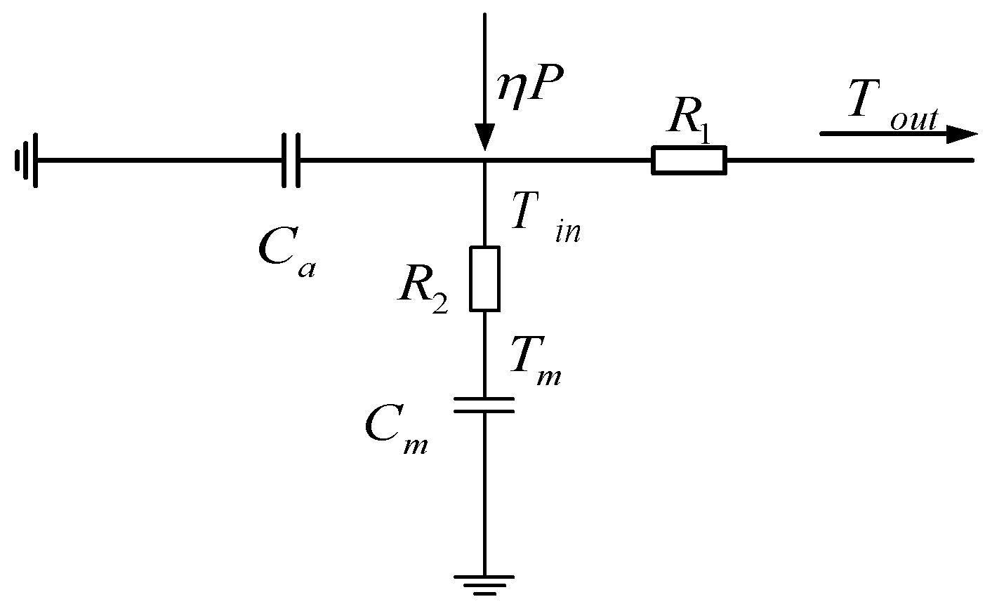
2.1. Thermodynamic Model of Single Air Conditioning

An equivalent thermal parameters (ETP) model of air conditioning is shown in Figure 1 [24].

$C_a$: air heat capacity ($J/°C$);

$C_m$: mass heat capacity ($J/°C$);

$P$: rated power for air conditioning ($W$);

$\eta$: energy efficiency ratio of air conditioning;

$R_1$: ambient thermal resistance ($°C/W$);

$R_2$: mass thermal resistance ($°C/W$);

$T_{out}$: ambient temperature ($°C$);

$T_{in}$: air temperature inside the house ($°C$);

$T_m$: mass temperature inside the house ($°C$);

Based on the Newton’s cooling law [18,19], the ETP model is simplified to construct a thermodynamic model of a single air conditioning [18,19]. Equation (1) is the thermodynamic model of an air conditioning in a closed state and Equation (2) is the thermodynamic model of an air conditioning in an operating state:

$$T_{in}^{t+1}=T_{out}^{t+1}+(T_{in}^t-T_{out}^{t+1}){\epsilon }^{\Delta t}$$

(1)

$$T_{in}^t=T_{out}^{t+1}-\eta P/UA+[T_{in}^{t+1}-(T_{out}^{t+1}-\eta P/UA)]{\epsilon }^{\Delta t}$$

(2)

where:

${\epsilon }^{\Delta t}$: heat dissipation function, $\epsilon {=\mathrm{e}}^{\frac{-1}{RC}}$;

$t$: time (minute);

$\Delta t$: time step (1 min);

$UA$: standby heat loss coefficient ($W/°C$);

$C$: equivalent heat capacity ($J/°C$);

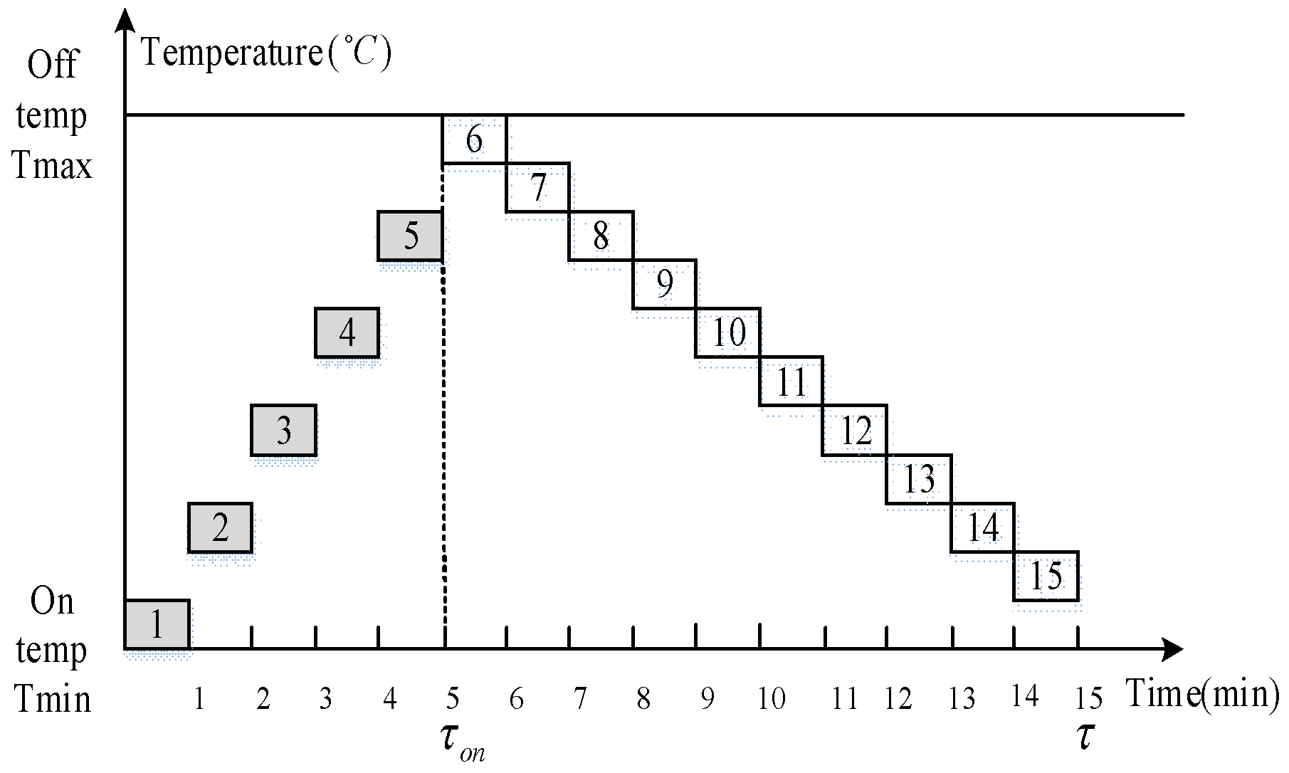
2.2. A State-Queuing Model of Aggregate Air Conditionings

When demand-side resources participate in tracking renewable energy output, user comfort should not be affected. Thus, we convert the user’s usage requirements into parameters and incorporate them into the model [25].

We set the temperature range required by users to be $\left[T_{min},T_{max}\right]$. Combined with the temperature range, Equations (3) and (4) can be derived from Equations (1) and (2) if an air conditioning is in the heating mode. $\overline{P}$ is the average power of an air conditioning.

$$T_{min}=T_{out}+(T_{max}-T_{out}){\epsilon }^{{\tau }_{off}}$$

(3)

$$T_{min}=T_{out}-\eta \overline{P}/UA+\left(T_{max}-T_{out}+\eta \overline{P}/UA\right){\epsilon }^{{\tau }_{on}}$$

(4)

$$\tau ={\tau }_{on}+{\tau }_{off}$$

(5)

Equation (5) represents a cycling time of aggregate air conditionings, where ${\tau }_{on}$ is an “on” period and ${\tau }_{off}$ is an “off” period.

There are n air conditionings divided into $\tau$ groups, one of which operates without interference, as shown in Figure 2. The state of the air conditioning changes once per minute. The air conditionings are turned on in the first ${\tau }_{on}$ minutes and turned off in the next ${\tau }_{off}$ minutes. Each state of the air conditionings corresponds to a temperature range.

Assuming that the control period is 15 min, the “on” period is five minutes and the “off” is 10 min. The state distribution of the $\tau$ groups of loads in one control period is shown in

Table 1. Fifteen groups of load temperature state distributions.

State	1	2	3	4	5	6	7	8	9	10	11	12	13	14	15	on
1	1	2	3	4	5	6	7	8	9	10	11	12	13	14	15	5
2	2	3	4	5	6	7	8	9	10	11	12	13	14	15	1	5
3	3	4	5	6	7	8	9	10	11	12	13	14	15	1	2	5
4	4	5	6	7	8	9	10	11	12	13	14	15	1	2	3	5
5	5	6	7	8	9	10	11	12	13	14	15	1	2	3	4	5
6	6	7	8	9	10	11	12	13	14	15	1	2	3	4	5	5
7	7	8	9	10	11	12	13	14	15	1	2	3	4	5	6	5
8	8	9	10	11	12	13	14	15	1	2	3	4	5	6	7	5
9	9	10	11	12	13	14	15	1	2	3	4	5	6	7	8	5
10	10	11	12	13	14	15	1	2	3	4	5	6	7	8	9	5
11	11	12	13	14	15	1	2	3	4	5	6	7	8	9	10	5
12	12	13	14	15	1	2	3	4	5	6	7	8	9	10	11	5
13	13	14	15	1	2	3	4	5	6	7	8	9	10	11	12	5
14	14	15	1	2	3	4	5	6	7	8	9	10	11	12	13	5
15	15	1	2	3	4	5	6	7	8	9	10	11	12	13	14	5
16	1	2	3	4	5	6	7	8	9	10	11	12	13	14	15	5

. ${\tau }_{on}/\tau$ represents the proportion of air conditionings in the “on” state. It can be found that the proportion is constant if the temperature range is not changed during the control period. The load capacity of air conditionings during the x-period is shown by Equation (6).

$$P_x=\frac{{\tau }_{on}}{\tau }nP$$

(6)

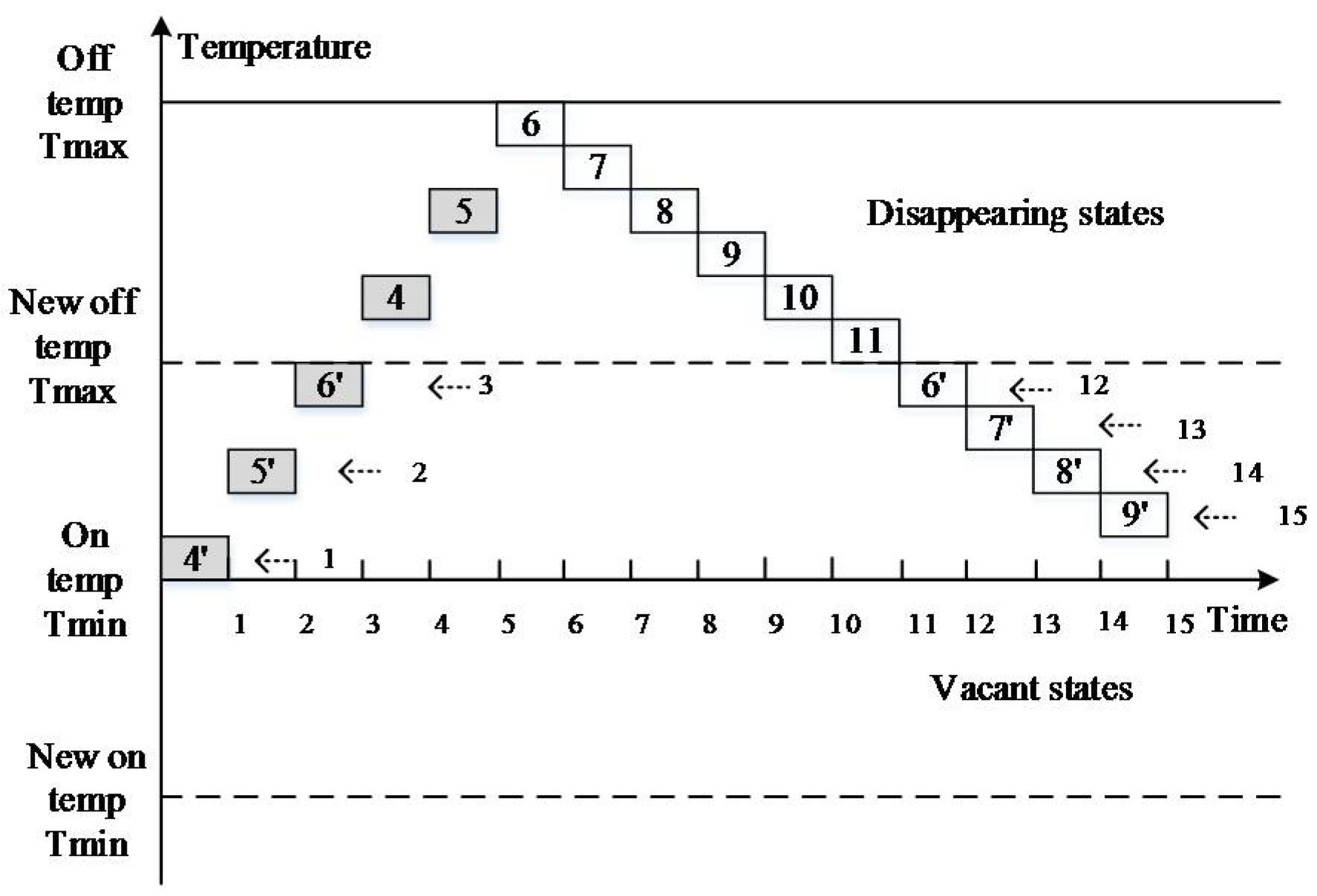
2.3. Characteristics of the State-Queuing Model

The state-queuing aggregation model of the air conditionings per minute is constant without the temperature range setting changing. However, the temperature setting range sometimes has to change in practice. Therefore, the relationship between the temperature setting range and the output characteristics of the state-queuing model needs to be analyzed. The temperature range is divided into ${\tau }_{off}$ = 10 segments and the temperature interval of each segment is called a temperature unit. When the control temperature range is lowered by six units, that is, the temperature space becomes $\left[T_{min}-\frac{3}{5}(T_{max}-T_{min}),T_{max}-\frac{3}{5}(T_{max}-T_{min})\right]$, the state changing process of a group is shown in Figure 3. From Figure 3, it can be seen that some states of the air conditionings have disappeared and become vacant. There is a state transition phenomenon. State 1 is changed into state 4; state2 is changed into state 5; state 3 is changed into state 6; states 4–11 disappear; state 12 is changed into state 6; state 13 is changed into state 7; state 14 is changed into state 8; state 15 is changed into state 9; and states 10–15 appear vacant.

Table 2. Fifteen groups of load state distributions after temperature adjustment.

State	1	2	3	4	5	6	7	8	9	10	11	12	13	14	15	on
1	4	5	6	off	off	off	off	off	off	off	off	6	7	8	9	2
2	5	6	7	off	off	off	off	off	off	off	6	7	8	9	10	1
3	6	7	8	6	off	off	off	off	off	6	7	8	9	10	11	0
4	7	8	9	7	off	off	off	off	6	7	8	9	10	11	12	0
5	8	9	10	8	6	off	off	6	7	8	9	10	11	12	13	0
6	9	10	11	9	7	off	6	7	8	9	10	11	12	13	14	0
7	10	11	12	10	8	6	7	8	9	10	11	12	13	14	15	0
8	11	12	13	11	9	7	8	9	10	11	12	13	14	15	1	1
9	12	13	14	12	10	8	9	10	11	12	13	14	15	1	2	2
10	13	14	15	13	11	9	10	11	12	13	14	15	1	2	3	3
11	14	15	1	14	12	10	11	12	13	14	15	1	2	3	4	5
12	15	1	2	15	13	11	12	13	14	15	1	2	3	4	5	7
13	1	2	3	1	14	12	13	14	15	1	2	3	4	5	6	9
14	2	3	4	2	15	13	14	15	1	2	3	4	5	6	7	9
15	3	4	5	3	1	14	15	1	2	3	4	5	6	7	8	10
16	4	5	6	4	2	15	1	2	3	4	5	6	7	8	9	9
17	5	6	7	5	3	1	2	3	4	5	6	7	8	9	10	8
18	6	7	8	6	4	2	3	4	5	6	7	8	9	10	11	5
19	7	8	9	7	5	3	4	5	6	7	8	9	10	11	12	4
20	8	9	10	8	6	4	5	6	7	8	9	10	11	12	13	2
21	9	10	11	9	7	5	6	7	8	9	10	11	12	13	14	1

shows the distribution of load states after six units of temperature settle down. The shaded part indicates that the air conditioning’s state is on. It can be seen that the proportion of air conditionings in the “on” state is no longer equal in each time period. The load of air-conditioning fluctuates during a control period. If the air conditionings sustain operation for multiple control periods, it is not difficult to determine that such load fluctuations are periodic. The core of this phenomenon is that air conditionings which meet the new temperature range are insufficient, thus, a transition period is needed. When the new temperature range has air conditionings in all temperature states, it reaches a stable stage. However, ${\tau }_{on}/\tau$ in each time period is no longer equal, that is, the proportion of air conditionings in the “on” state are no longer equal.

Figure 4 shows the air conditionings’ load curves when the temperature range moves up and down six units, respectively. The red curve represents an upward change in the temperature, and the blue curve represents a downward change in the temperature. Different temperature adjustments correspond to different load curves. The diversity of load curves can remain abundant. In practical applications, this can be achieved only by knowing the temperature range instead of adjusting the temperature if a certain fluctuating load curve is obtained. The corresponding loads are selected according to the load temperature state distribution table. Different initial temperature distributions correspond to different load curves. If such a load curve is regarded as a basic signal, a target signal can be obtained by superimposing basic signals of different amplitudes and different frequencies according to the principle of signal decomposition. Therefore, we can make use of the periodic fluctuations of the air conditioning load to achieve renewable energy output tracking.

3. Control Algorithm

Based on the above, the load curves of the aggregate air conditionings can be controlled by changing the initial temperature distribution of the air conditionings. The corresponding load curve can be extended by one cycle to obtain a periodically fluctuating load curve. Therefore, a virtual load curve set Q is established based on the controllable air conditioning loads’ temperature states’ distribution table. The load curves are used as the basic signals, and the renewable energy output is used as the target signal. According to the signal decomposition principle, signals with different amplitudes and frequencies can be superimposed to obtain the desired target signal, that is, in accordance with the actual demand of renewable energy consumption, we select the appropriate load curves to superimpose in order to track renewable energy output. This control algorithm tracks the energy output in each period. The redistribution of load resources at each stage can effectively mobilize the load resources while maintaining the state diversity of the load resources. Load control is more accurate because of adequate load status.

The first part of this section establishes the objective function based on the actual tracking requirements; the objective function is divided into two parts: the solving coefficients and the target optimization. The second part describes in detail that how to solve the unknown coefficients of the objective function with fixed load curves combination, so as to minimize the objective function. The third part expands the scope of the solution. Under the condition that the load curve combination is unknown, the optimal load curve combination is selected in the Q, so that the objective function is minimized.

Thus, this paper establishes a renewable energy output tracking control algorithm based on the state-queuing model of thermostatically controlled loads.

3.1. Objective Function

The error during the tracking process is the difference $\gamma$ between the renewable energy output and the aggregate air conditioning loads, as shown in Equation (7). Then we establish an objective function with the goal of minimizing overall tracking error, as described by Equations (8) and (9):

$$Y_o=Y_s+\gamma$$

(7)

$$F=\min {\displaystyle \sum _{j=1}^{\tau }{[Y_o(j)-Y_s(j)]}^2}$$

(8)

$$Y_s(j)={\displaystyle \sum _{i=1}^m\beta (i)Y(j)(i)}$$

(9)

$$m<\tau$$

The cycling time of the tracking process is $\tau$. $Y_o\in R^{\tau \times 1}$ is the renewable energy output during $\tau$ minutes. The fitting vector is $Y_s\in R^{\tau \times 1}$, which represents the aggregate air conditioning loads within $\tau$ minutes. Load curve combination is $Y\in R^{\tau \times m}$. It represents the m groups of selected load curves. The coefficient $\beta \in R^{m\times 1}$ is the multiplier of the m groups load curves, representing the number of controlled air conditionings in each group.

$Y_s$ is a $\tau \times m$ order equation. $\tau$ is the number of equations and m is the number of unknown variables. If there are sufficiently abundant load curves in set Q, the objective function is essentially an over-determined equation, i.e., $m<\tau$. The least square method is an effective method for solving over-determined equations. Therefore, this paper uses the least square method to solve unknown coefficients.

Actually, the fitted value of the controlled loads should not exceed the actual renewable energy output so as to make no burden on the power grid, and $Y_s$ should be less than $Y_o$ (i.e., load deviation $\gamma >0$). Moreover, the multiplier of the load curve represents the required number of loads for each group and must be non-negative. The constraints can be described as follows:

$$\beta \left(i\right)\ge 0,i\in [1,m]$$

(10)

$$Y_s\left(j\right)\le Y_o\left(j\right),j\in [1,\tau ]$$

(11)

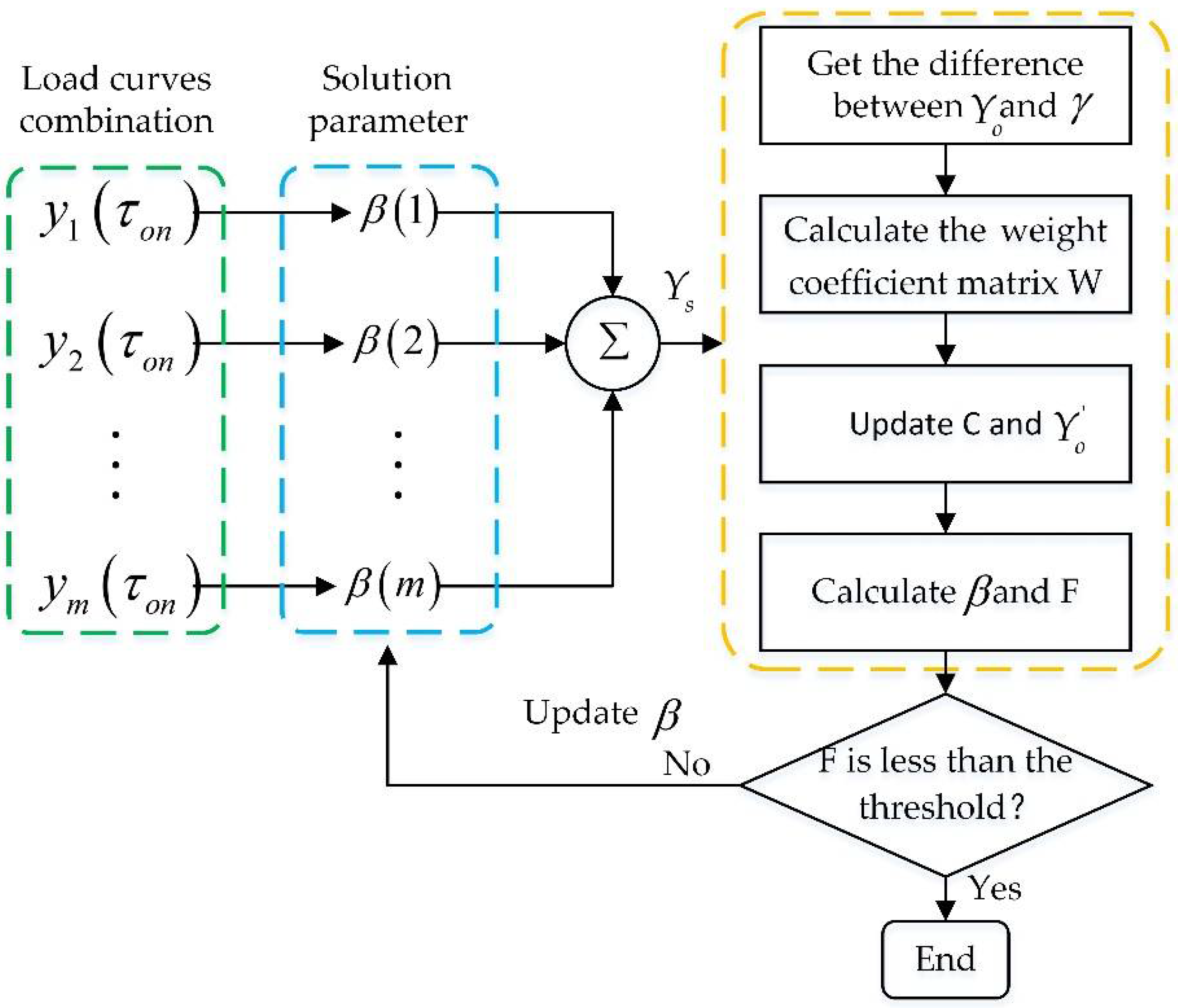
3.2. Solution of the Objective Function

Since the actual data is heteroskedastic, this paper uses the weighted least squares method to solve the objective function and eliminate the influence of heteroscedasticity. By doing so, the solution parameter $\beta$ satisfies the Markov estimation [26,27]. Compared with the basic least squares method, the weighted least squares method adds a weighting factor $\omega$ to the objective function, which is the reciprocal of the square of the load deviation at the corresponding point. The improved objective function and $\omega$ are:

$$\omega \left(j\right)=\frac{1}{{\left(Y_o\left(j\right)-Y_s\left(j\right)\right)}^2},j\in [1,\tau ]$$

(12)

$$\{\begin{array}{c}F=min{\displaystyle \sum _{j=1}^{\tau }\omega (j){[Y_o(j)-Y_s(j)]}^2}\\ \omega \left(j\right)=\frac{1}{{\left(Y_o\left(j\right)-Y_s\left(j\right)\right)}^2},j\in [1,\tau ]\\ Y_s(j)={\displaystyle \sum _{i=1}^m\beta (i)Y(j)(i)}\\ \beta \left(i\right)\ge 0,i\in [1,m]\\ Y_s\left(j\right)\le Y_o\left(j\right),j\in [1,\tau ]\\ m<\tau \end{array}$$

(13)

The weight coefficient matrix W is:

$$\left(\begin{array}{cccc}{\omega }_1& 0& \cdots & 0\\ 0& {\omega }_2& \cdots & 0\\ ⋮& ⋮& ⋮& ⋮\\ 0& 0& \cdots & {\omega }_{\tau }\end{array}\right)$$

(14)

Then, using Equation (14), the objective function is recast as:

$$\begin{array}{l}F=minW{\left(Y_o-Y_s\right)}^2=min{\left(\sqrt{W}{Y}_o-\sqrt{W}{Y}_s\right)}^2\\ =min{\left(Y_o^{\prime }-Y_s^{\prime }\right)}^2=min{\left(Y_o^{\prime }-C·B\right)}^2\end{array}$$

(15)

$$Y_s=Y·\left(\begin{array}{c}{\beta }_1\\ {\beta }_2\\ ⋮\\ {\beta }_m\end{array}\right)=Y·B$$

(16)

$$C=\sqrt{W}Y$$

(17)

where $Y_o^{\prime }$ and $Y_s^{\prime }$ are, respectively, the target vector and fitting vector considering the weight coefficient W. $Y_s$ can be recast as Equation (16). In addition the load curve combination $Y$ is treated as the coefficient matrix.

Finally, a new parameter relationship can be obtained, as shown in Equations (18) and (19):

$$\sqrt{W}{Y}_o=\sqrt{W}Y·B+\gamma$$

(18)

$$Y_o^{\prime }=Y_s^{\prime }+\gamma =C·B+\gamma$$

(19)

The process of solving the objective function with weight coefficients is shown in Figure 5. At the beginning, $\beta$ needs to be initialized. In order to improve the convergence rate of the solution process, the initial $\beta$ is set as a weighted least squares solution with inequality constraints and the weight coefficient is initialized to 1. It can be seen that the load curves are respectively multiplied with the corresponding $\beta$, and the fitting curve $Y_s$ is obtained by superposition. Next, $Y_s$ is compared with the target curve $Y_o^{\prime }$ to obtain the load deviation and the weight coefficient matrix W. Then, update the matrix $C$ and the target vector $Y_o^{\prime }$ according to W. Finally, we calculate the least squares solution of the objective function F with constraints and determine whether the end condition is satisfied. If not, we update $\beta$ using the value obtained by this cycle calculation and repeat the above process.

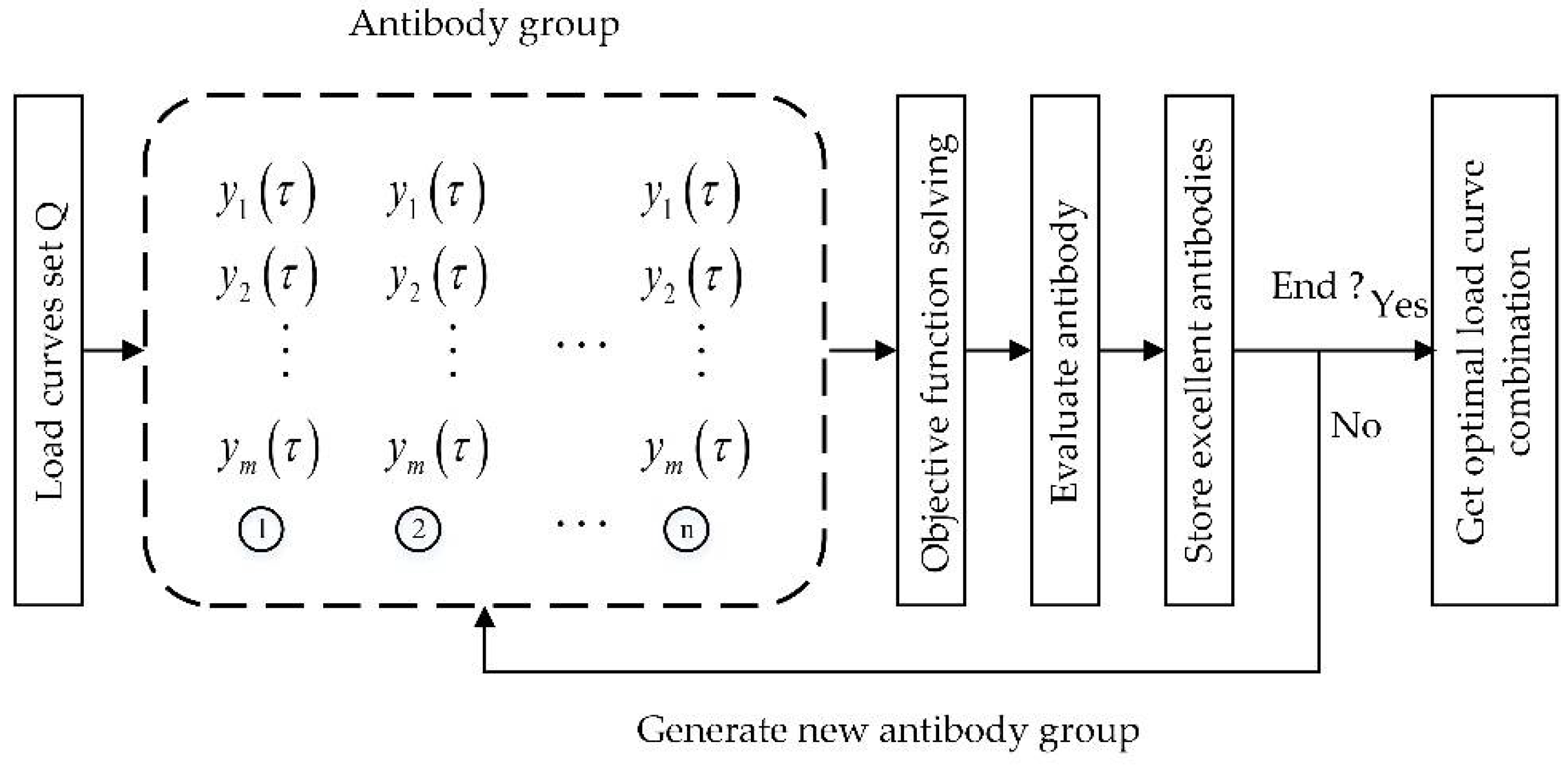
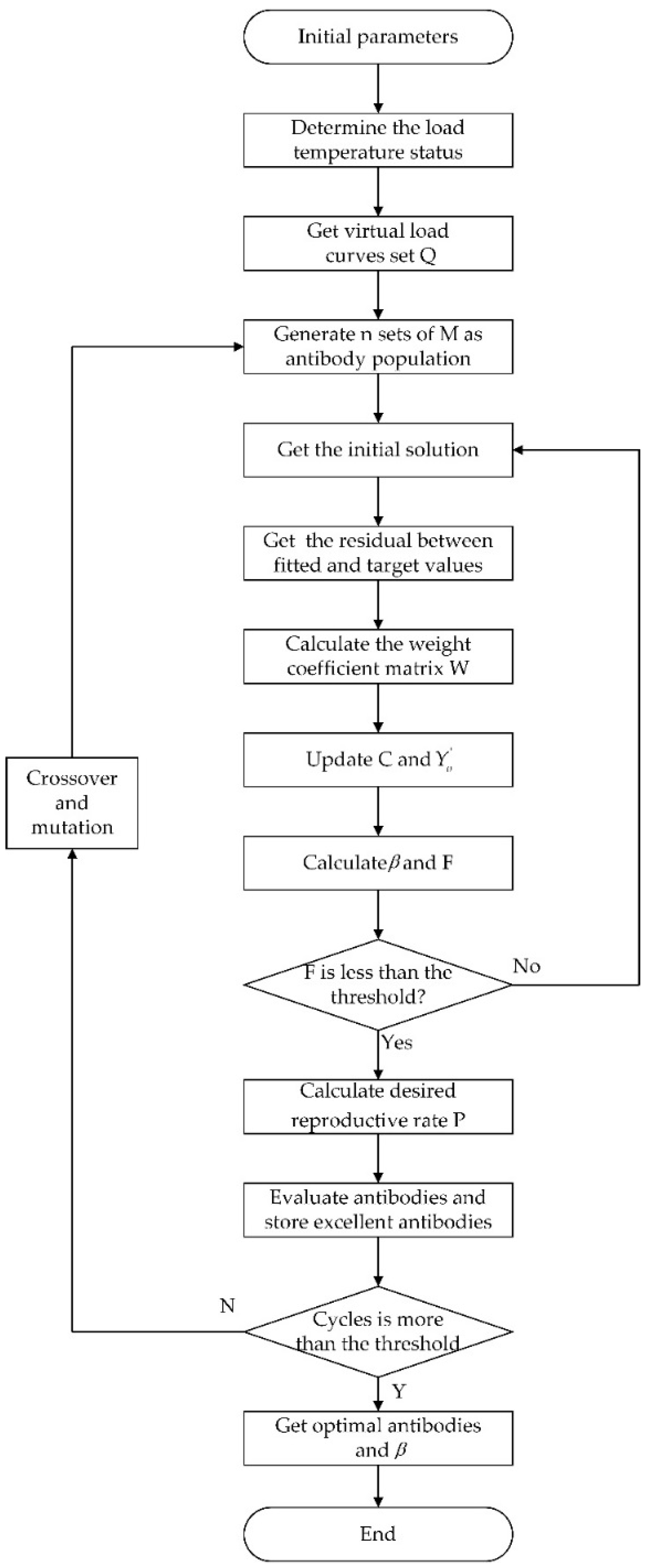
3.3. The Process of Optimization

The coefficient $\beta$ can be obtained by solving the above objective function. The number of load curves selected from Q is m. Since the number of load curves in Q is much larger than m, the next problem is how to select appropriate curves from the set so that the objective function is minimized. By the optimized solution algorithm, the optimal load curve combination and $\beta$ can be obtained.

Compared with other optimization algorithms, the artificial immune algorithm has good parallelism and can be perfectly combined with other algorithms. Additionally, if a comprehensive evaluation system is used to evaluate the individuals involved in optimization, the generation of new individuals will be more complex. This can ensure the diversity of the individuals involved in optimization, and avoid falling into the local optimal, thus, the overall convergence of the algorithm is excellent and the operation efficiency is high [28,29,30,31,32,33].

Figure 6 shows the process of objective function optimization. The combination of the load curves is set to M and the number of load curves contained is m. Firstly, based on the load curve set Q, an antibody population with size n is randomly generated, and each antibody represents a load curve combination M. Then, the objective function solution model is used to obtain $\beta$. We then calculate the antibody evaluation coefficient and evaluate the antibody according to $\beta$. Excellent antibodies are used as the parent antibodies and are preserved. Then we determine whether the optimization end condition is met. If the iteration continues, a good antibody is used to generate a new antibody population through crossover and mutation methods until the best load curve combination is obtained.

In this paper, each antibody is evaluated by comparing the individual’s desired reproductive rate. In Equation (20), $\alpha$ is a constant and reproductive rate P is affected by antibody concentration and antibody affinity. $A_v$ is the affinity between the antibody and antigen, which takes the reciprocal of the objective function F. As shown in Equation (21), the smaller the objective function is, the higher the affinity becomes. This indicates that the higher the antibody’s recognition of the antigen is, the better the selected combination M of load curves is. $C_v$ is the antibody concentration, which represents the proportion of similar antibodies in the antibody population. In other word, it is the similar degree between the different load curve combinations M. Obviously, a high antibody concentration will increase the individual reproductive rate, but it is not conducive to the diversity of antibody population. Thus, Equation (21) plays a role in inhibiting high-concentration individuals and ensures antibody diversity:

$$P=\alpha \frac{A_v}{{\displaystyle \sum A_v}}+\left(1-\alpha \right)\frac{C_v}{{\displaystyle \sum C_v}}$$

(20)

$$A_v=\frac{1}{F}=\frac{1}{{\displaystyle \sum _{j=1}^{\tau }w\left(j\right){\left[y_o\left(j\right)-y_s\left(j\right)\right]}^2}}$$

(21)

$C_v$ is obtained by the affinity $S_{v,s}$ shown in Equations (22) and (23). In Equation (23), $k_{v,s}$ is the number of the same elements between the antibody v and s; the length of the antibody is m:

$$C_v=\frac{1}{n}{\displaystyle \sum _{i\in n}{S}_{v,s}}$$

(22)

$$S_{v,s}=\frac{k_{v,s}}{m}$$

(23)

Figure 7 shows the overall flow of the proposed algorithm. According to the temperature state distribution table of air conditioning loads, a virtual load curve set Q is obtained. On this basis, the artificial immune algorithm is used to select the optimal load curve combination. At the same time, the target function is solved by the weighted least square method, and $\beta$ is obtained. The fitting curve is obtained by optimal load curves and $\beta$, which can ensure the minimum load deviation from the target curve. The algorithm can be effectively applied to track renewable energy output.

4. Experimental Results and Simulation

In this section, we obtain the performance of the proposed control algorithm in three parts. Firstly, we set the target value and simulation parameters. We use the 24-h wind power output data as the target value. Secondly, according to control algorithm in Section 3, we use a real wind power trajectory within 15 min to simulate in detail, and a tracking trajectory over the period of a day is provided. Finally, this paper analyzes the simulation error and the performance of the control algorithm.

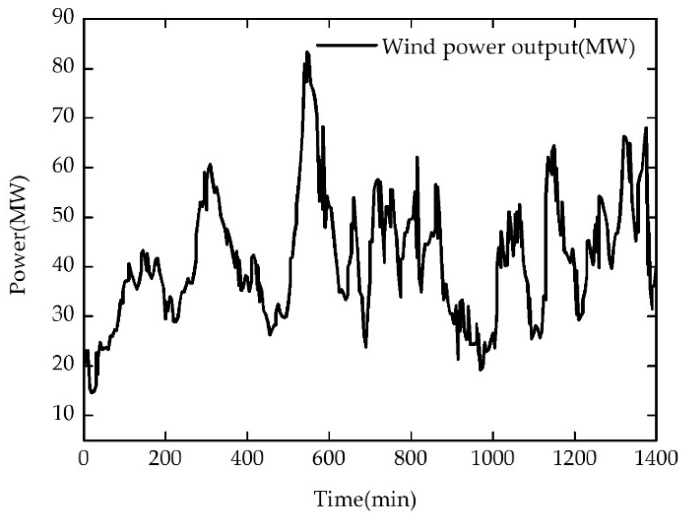
4.1. Target Value and Simulation Parameter Setting

The wind power output data was obtained from a wind farm with an installed capacity of 90 MW. The wind power trajectory is shown in Figure 8.

According to Section 3, the initial parameters of the control algorithm are shown in

Table 3. Initialization parameters.

Parameters	Values	Formula
Population size	50	—
Memory capacity	15	—
Cycle times	50	—
Crossover probability	0.4	—
Mutation probability	0.5	—
Diversity parameter	0.95	—
Reproductive rate	—	Equation (16)
$A_v$	—	Equation (13)
$S_v$	—	Equation (15)
Antibody concentration	—	Equation (14)

.

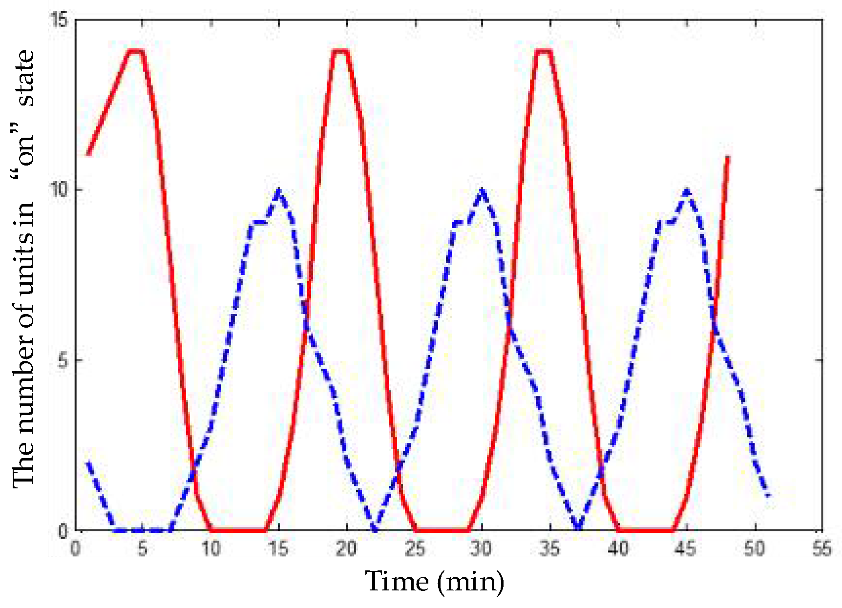
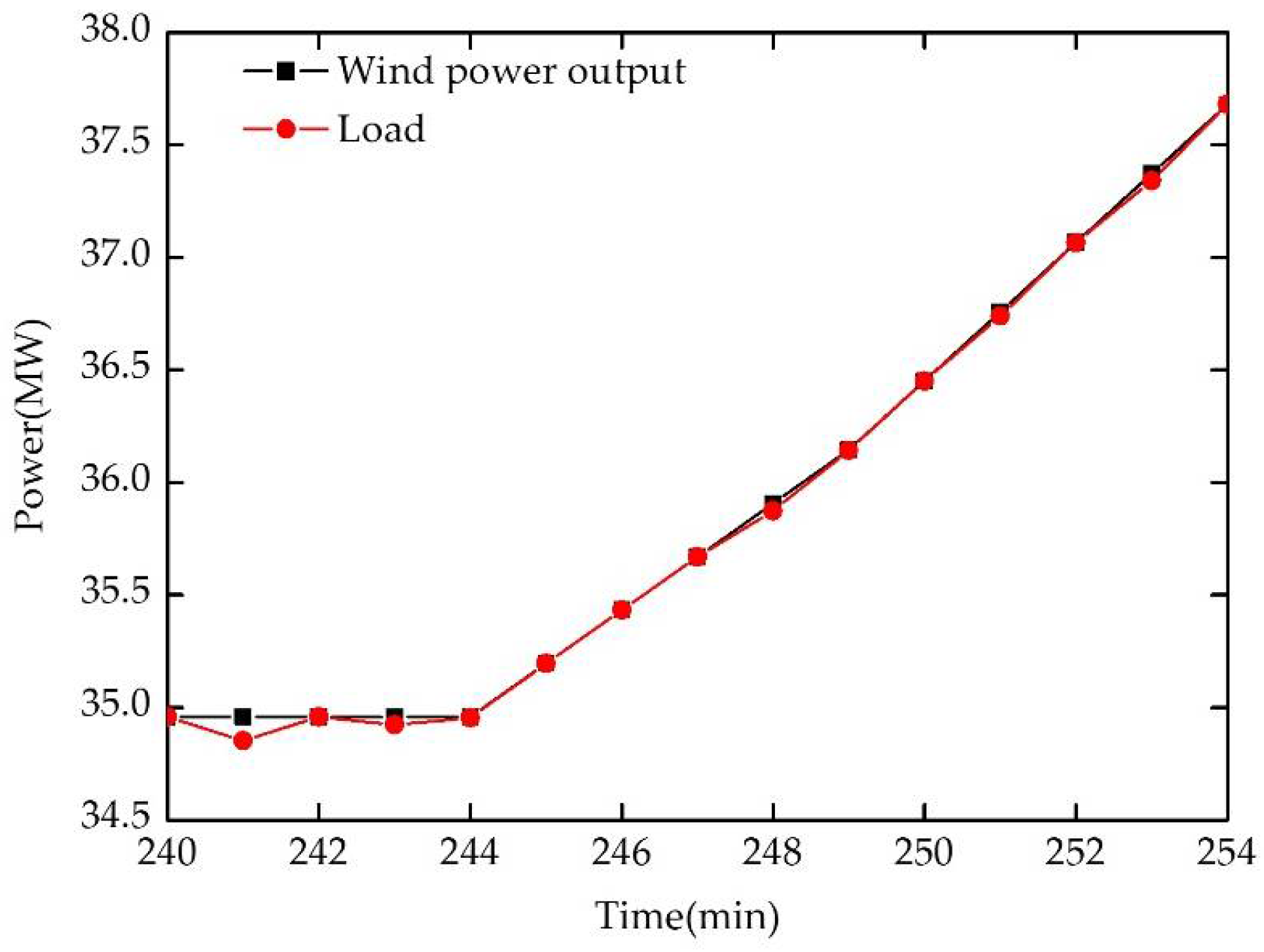
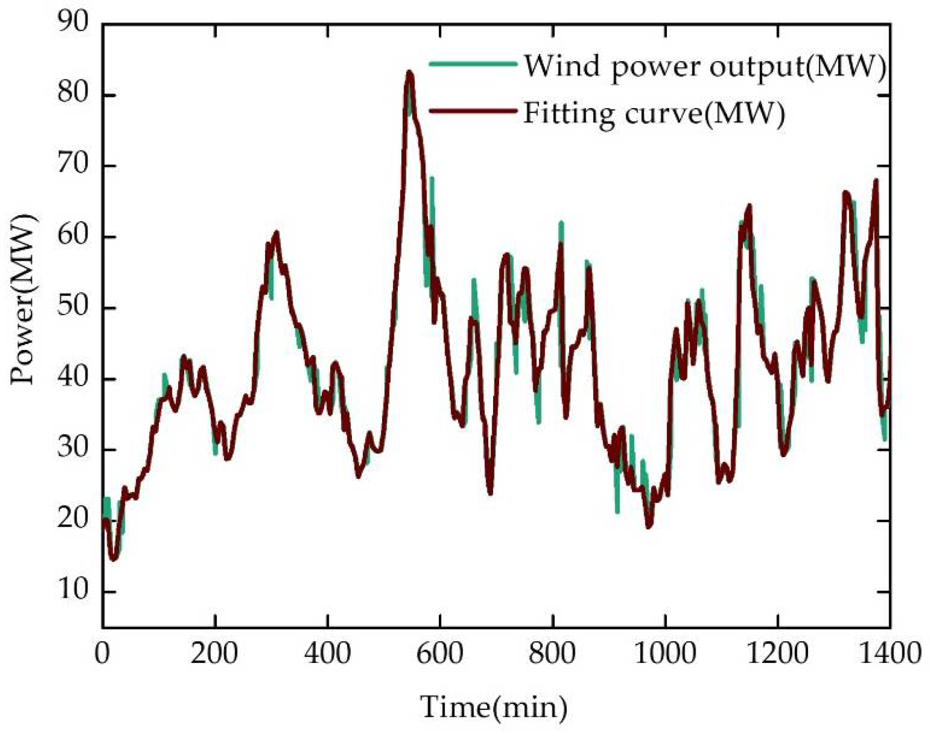
4.2. Load Control and Tracking Results

Based on the control algorithm in Section 3, the optimal load curve combination can be obtained from the load curve set. The simulation control period is set as 15 min. Taking the tracking from 4:00 a.m. to 04:15 a.m. as an example,

Table 4. Load curve amplitude.

Time	Groups
	4	9	20	21	24	26	58	67	77	83
1	6	14	0	0	0	0	2	9	4	1
2	11	12	0	0	0	0	3	10	2	0
3	14	8	0	0	0	1	5	9	1	0
4	14	4	0	0	1	3	7	8	0	0
5	12	1	0	1	3	6	9	5	1	0
6	8	0	1	3	6	11	9	4	2	0
7	4	0	3	6	11	14	10	2	3	0
8	1	0	6	11	14	14	9	1	5	0
9	0	0	11	14	14	12	8	0	7	0
10	0	0	14	14	12	8	5	1	9	1
11	0	1	14	12	8	4	4	2	9	3
12	0	3	12	8	4	1	2	3	10	5
13	0	6	8	4	1	0	1	5	9	7
14	1	11	4	1	0	0	0	7	8	8
15	3	14	1	0	0	0	1	9	5	9

shows the load curve combination calculated by the control algorithm. The value of coefficient vector $\beta$ is [0.0282, 0, 0.0049, 0, 0, 0.0154, 1.556, 1.5218, 1.5829, 0.0022]. This means that it needs 14, 0, 2, 0, 0, 8, 778, 761, 792 and 1 groups, respectively, if the unit power of a group of loads is 2 kW.

Figure 9 shows the fitted load curve from 4:00 a.m. to 04:15 a.m. After entering the next control period, the air conditioning loads in the last period will no longer be controlled and it will work at its original temperature settings. The diversity of the air conditioning temperature states can be kept abundant. The wind power curve should be handled in advance. After reducing the basic consumption of other loads, the remaining part will be tracked by air conditioning loads. The fitted load curve can fit well with the wind power curve. This indicates that the algorithm proposed in this paper is effective.

The 24-h wind power output tracking is shown in Figure 10. From Figure 10, the wind power trajectory over a long period can also be tracked well and effectively.

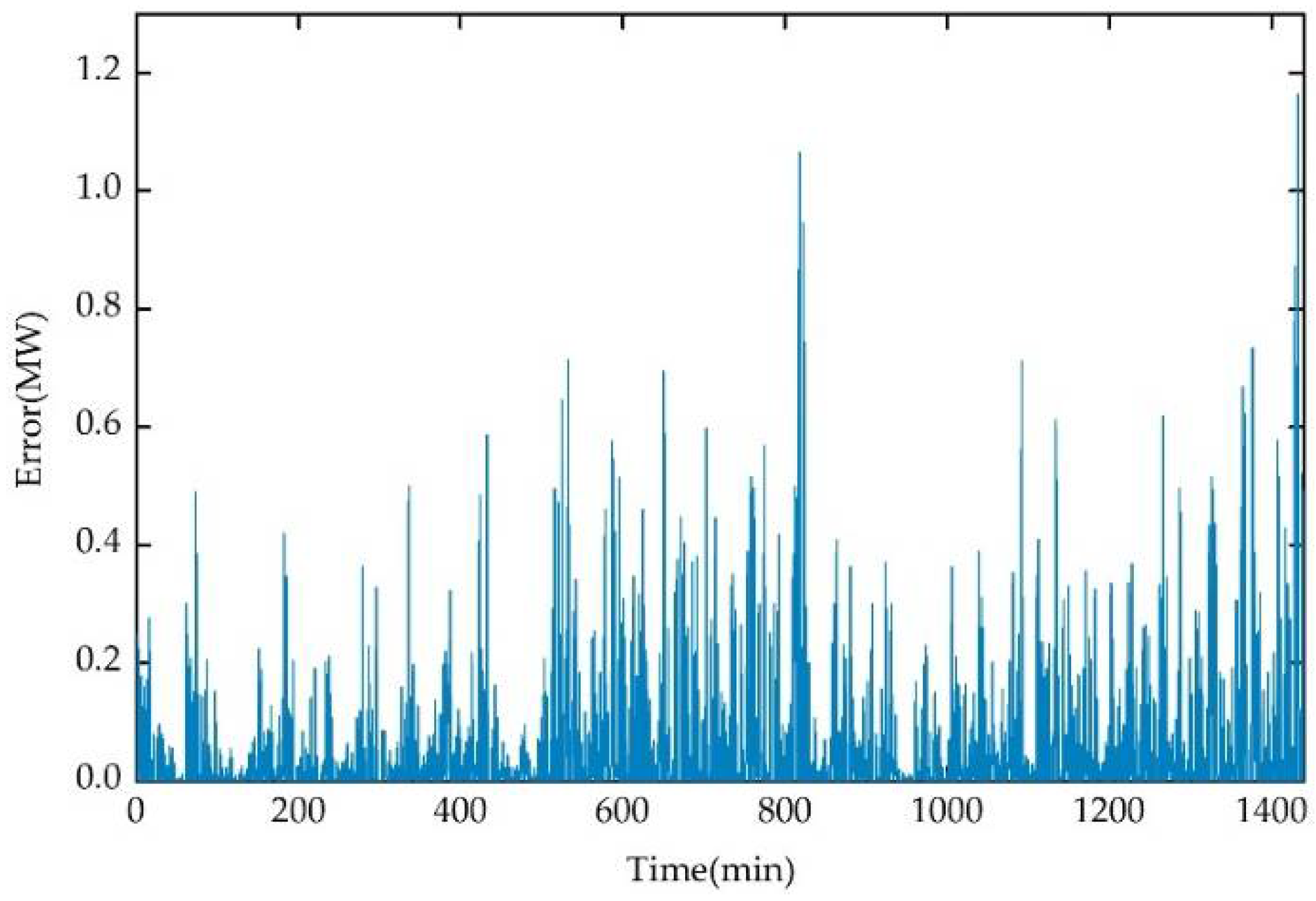
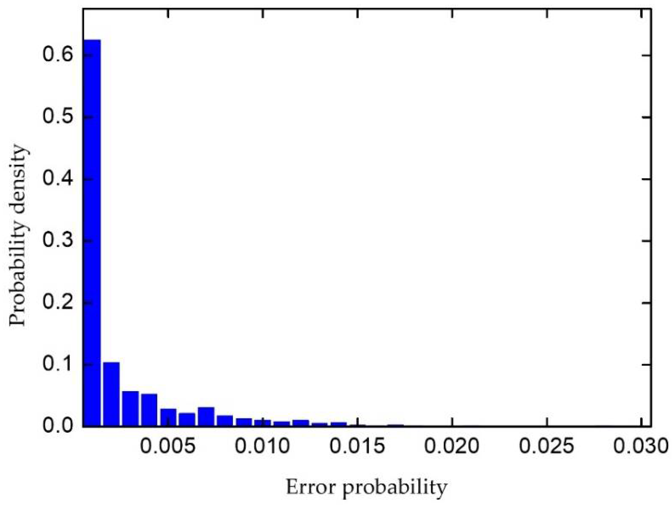
4.3. Error Evaluation of Experimental Results

Figure 11 shows the tracking error for 24 h. Figure 12 shows the error probability density for wind power tracking. As can be seen, the error probability is mostly concentrated around 0, and the error probability distribution in [0, 0.0007] is up to 60%, the maximum error range within 3%. Therefore, the wind tracking control algorithm proposed in this paper has an ideal accuracy rate. In addition, compared with other tracking methods, the algorithm has a more convenient control process and the diversity of loads can be maintained. Bashash et al. [23] proposed controlling the loads by adjusting the temperature settings of the air conditioning loads, whose error probability is controlled within 5%. However, when the load similarity is high, fine-tuning the temperature settings will cause the loss of load diversity, and the cluster load will fluctuate greatly. In addition, this method is a process of closed-loop control. It is necessary to adjust the control signal in real-time and constantly correct it. The information feedback channel is indispensable and the control cost is too high. However, our phased plan control method does not require real-time regulation of the load. Compared with [23], the accuracy of our algorithm is higher with the error controlled within 3%. The diversity of load states are always abundant and it makes the control process more stable. At the same time, our method is more convenient to realize. It can be used to track the output of renewable energy, which is of great significance to load control decision-making.

5. Discussion

Based on the state-queuing model, this paper presents a control algorithm to consume renewable energy and track renewable energy output. Firstly, a state-queuing model of air conditioning loads is developed. The aggregate air conditioning load fluctuates after the distribution of the air conditioning temperature states change. Then, we establish a virtual load curves set based on the state-queuing model and regard the load curves as basic signals, with the renewable energy output as the target signal. Secondly, by artificial immune algorithm optimization and weighted least squares, the control algorithm can select and calculate the optimal load curves for linear combination. Finally, the performance of the renewable energy output tracking control algorithm is simulated based on the 24-h wind power output of a wind farm. Simulation results show that the fitting curve can track the wind power output curve well and the tracking control algorithm proposed in this paper has an ideal accuracy rate. In addition, the error probability can be controlled within 3%. The tracking control algorithm proposed in this paper can be applied in tracking and consuming renewable energy and it provides a new idea for demand-side loads to participate in renewable energy consumption.

In order to make the demand-side loads involved in scheduling coordinate with each other well, our further work will focus on the combination of different kinds of demand-side loads to enhance the model stability and the prediction of the load curves.

References

1. Su, H.; Zhang, T.; Qian, L.; Wang, Z.; Cai, Q.; Wang, B. Consensus control strategy of inverter air conditioning group for renewable energy consumption based on distributed adaptive system. In Proceedings of the 2017 IEEE 2nd Information Technology, Networking, Electronic and Automation Control Conference (ITNEC), Chengdu, China, 15–17 December 2017; pp. 92–96. [Google Scholar]
2. Mahdavi, N.; Braslavsky, J.H.; Seron, M.M. Model predictive control of distributed air-conditioning loads to compensate fluctuations in solar power. IEEE Trans. Smart Grid. 2017, 8, 3055–3065. [Google Scholar] [CrossRef]
3. Al Jabery, K.; Xu, Z.; Yu, W. Demand-side management of domestic electric water heaters using approximate dynamic programming. IEEE Trans. Comput.-Aided Des. Integr. Circuits Syst. 2017, 36, 775–788. [Google Scholar] [CrossRef]
4. Xu, Z.; Diao, R.; Lu, S. Modeling of electric water heaters for demand response: A baseline PED model. IEEE Trans. Smart Grid. 2014, 5, 2203–2210. [Google Scholar] [CrossRef]
5. Sossan, F.; Kosek, A.M.; Martinenas, S. Scheduling of domestic water heater power demand for maximizing PV self-consumption using model predictive control. In Proceedings of the 2013 IEEE Innovative Smart Grid Technologies Europe, Lyngby, Denmark, 6–9 October 2013; pp. 1–5. [Google Scholar]
6. Shah, J.J.; Nielsen, M.C.; Shaffer, T.S. Cost-optimal consumption-aware electric water heating via thermal storage under time-of-use pricing. IEEE Trans. Smart Grid. 2016, 7, 592–599. [Google Scholar] [CrossRef]
7. Kondoh, J.; Lu, N.; Hammerstrom, D.J. An Evaluation of the water heater load potential for providing regulation service. In Proceedings of the 2011 IEEE Power and Energy Society General Meeting, Detroit, MI, USA, 24–29 July 2011; Volume 26, pp. 1309–1316. [Google Scholar]
8. Pourmousavi, S.A.; Patrick, S.N.; Nehrir, M.H. Real-time demand response through aggregate electric water heaters for load shifting and balancing wind generation. In Proceedings of the 2014 IEEE PES General Meeting|Conference & Exposition, National Harbor, MD, USA, 27–31 July 2014; Volume 5, pp. 769–778. [Google Scholar]
9. Goya, T.; Senjyu, T.; Yona, A. Optimal operation of controllable load and battery considering transmission constraint in smart grid. In Proceedings of the 2010 Conference Proceedings, Singapore, 27–29 October 2010. [Google Scholar]
10. Liu, M.; Quilumba, F.L.; Lee, W.J. A collaborative design of aggregated residential appliances and renewable energy for demand response participation. IEEE Trans. Ind. Appl. 2015, 51, 3561–3569. [Google Scholar] [CrossRef]
11. Qingqi, Z.; Ming, L.; Huaguang, Z. Dispatching strategy of responsive load using ant colony algorithm. Proc. CSEE 2006, 26, 15–21. [Google Scholar]
12. Lingling, S.; Ciwei, G.; Jian, T. Load aggregation technology and its applications. Autom. Electr. Power Syst. 2017, 41, 159–167. [Google Scholar]
13. Melhem, F.Y.; Grunder, O.; Hammoudan, Z. Optimization and energy management in smart home considering photovoltaic, wind, and battery storage system with integration of electric vehicles. Can. J. Electr. Comput. Eng. 2017, 40, 128–138. [Google Scholar]
14. Takigawa, F.Y.K.; Fernandes, R.C.; Tenfen, D. Energy management by the consumer with photovoltaic generation: Brazilian market. IEEE Lat. Am. Trans. 2016, 14, 2226–2232. [Google Scholar] [CrossRef]
15. Wong, S.; Pinard, J.P. Opportunities for smart electric thermal storage on electric grids with renewable energy. IEEE Trans. Smart Grid. 2017, 8, 1014–1022. [Google Scholar] [CrossRef]
16. Iacovella, S.; Ruelens, F.; Vingerhoets, P. Cluster control of heterogeneous thermostatically controlled loads using tracer devices. IEEE Trans. Smart Grid. 2017, 8, 528–536. [Google Scholar] [CrossRef]
17. Soudjani, S.E.Z.; Abate, A. Aggregation and control of populations of thermostatically controlled loads by formal abstractions. IEEE Trans. Control Syst. Technol. 2015, 23, 975–990. [Google Scholar] [CrossRef]
18. Masuta, T.; Yokoyama, A. Supplementary load frequency control by use of a number of both electric vehicles and heat pump water heaters. IEEE Trans. Smart Grid. 2012, 3, 1253–1262. [Google Scholar] [CrossRef]
19. Ciwei, G.; Qianyu, L.; Yang, L. Bi-level optimal dispatch and control strategy for air-conditioning load based on direct load control. Proc. CSEE 2014, 34, 1546–1555. [Google Scholar]
20. Lu, N.; Chassin, D.P. A state-queueing model of thermostatically controlled appliances. IEEE Trans. Power Syst. 2004, 19, 1666–1673. [Google Scholar] [CrossRef]
21. Lei, Z.; Yang, L.; Ciwei, G. Improvement of temperature adjusting method for aggregated air-conditioning loads and its control stratergy. Proc. CSEE 2014, 34, 5579–5589. [Google Scholar]
22. Callaway, D.S. Tapping the energy storage potential in electric loads to deliver load following and regulation, with application to wind energy. Eng. Conver. Manag. 2009, 50, 1389–1400. [Google Scholar] [CrossRef]
23. Bashash, S.; Fathy, H.K. Modeling and control of aggregate air conditioning loads for robust renewable power management. IEEE Trans. Control Syst. Technol. 2013, 21, 1318–1327. [Google Scholar] [CrossRef]
24. Lu, N. An evaluation of the HVAC load potential for providing load balancing service. IEEE Tran. Smart Grid. 2012, 3, 1263–1270. [Google Scholar] [CrossRef]
25. Fanti, M.P.; Mangini, A.M.; Roccotelli, M.A. District energy management based on thermal comfort satisfaction and real-time power balancing. IEEE Trans. Autom. Sci. Eng. 2015, 12, 1271–1284. [Google Scholar] [CrossRef]
26. Lawson, C.L.; Hanson, R.J. Solving least square problems. Camb. Univ Pr. 1974, 77, 673–682. [Google Scholar]
27. Wenxian, Z.; Xing, F.; Jingnan, L. Weighted total least squares algorithm with inequality constraints. Acta Geod. Cartogr. Sin. 2014, 43, 1013–1018. [Google Scholar]
28. Wei, L.; Changdong, L.; Deren, S. Research on optimazation of unit commitment based on immune algorithm. Proc. CSEE 2004, 24, 241–245. [Google Scholar]
29. Liang, Z.; Song, R.; Lin, Q.A. Double-module immune algorithm for multi-objective optimization problems. Appl. Soft Comput. 2015, 35, 161–174. [Google Scholar] [CrossRef]
30. Lin, Q.; Chen, J.; Zhan, Z.H. A Hybrid Evolutionary Immune Algorithm for Multiobjective Optimization Problems. IEEE Trans. Evol. Comput. 2016, 20, 711–729. [Google Scholar] [CrossRef]
31. Peteghem, V.V.; Vanhoucke, M. An artificial immune system algorithm for the resource availability cost problem. Flex. Serv. Manuf. J. 2013, 25, 122–144. [Google Scholar] [CrossRef]
32. Bagheri, A.; Zandieh, M.; Mahdavi, I. An artificial immune algorithm for the flexible job-shop scheduling problem. Future Gener. Comput. Syst. 2010, 26, 533–541. [Google Scholar] [CrossRef]
33. Zhao, J.; Liu, Q.; Wang, W. A parallel immune algorithm for traveling salesman problem and its application on cold rolling scheduling. Inf. Sci. 2011, 181, 1212–1223. [Google Scholar] [CrossRef]
Figure 1. Air conditioning equivalent thermal parameter model.
Applsci 08 01099 g001
Figure 2. Load operation state diagram.
Applsci 08 01099 g002
Figure 3. Load state transition diagram.
Applsci 08 01099 g003
Figure 4. Load fluctuation curve.
Applsci 08 01099 g004
Figure 5. Objective function solving module.
Applsci 08 01099 g005
Figure 6. Optimization of objective function.
Applsci 08 01099 g006
Figure 7. Algorithm flow chart.
Applsci 08 01099 g007
Figure 8. Wind power output curve.
Applsci 08 01099 g008
Figure 9. Wind power tracking comparison.
Applsci 08 01099 g009
Figure 10. Twenty-four hour wind power output tracking.
Applsci 08 01099 g010
Figure 11. Distribution of the error value.
Applsci 08 01099 g011
Figure 12. Probability density distribution of the wind power tracking error.
Applsci 08 01099 g012