Energy Sharing for Interconnected Microgrids with a Battery Storage System and Renewable Energy Sources Based on the Alternating Direction Method of Multipliers


Abstract
:1. Introduction
- (1)
- An energy sharing structure is proposed to integrate the neighboring MGs into an energy sharing zone. Besides, a virtual entity called ESP, which acts as an agent for multiple MGs, is introduced to minimize power loss cost.
- (2)
- Based on the framework of ADMM, a distributed optimal scheduling model and a two-level iterative algorithm for the MGs and ESP in coalition are proposed, which minimize the total operation cost including purchasing electricity cost, energy storage cost and power loss cost in coalition. The power loss cost can be decreased by the proposed method effectively.
- (3)
- An energy sharing framework at the distribution network level is proposed. Through bidirectional interaction between MGs and ESP, the optimal scheduling can be achieved until the expected exchange power decided by MGs is equal to the adjusted expected exchange power decided by ESP. During the optimization, the shared information is limited to expected exchange power, which protects the privacy of MGs and ESP.
- (4)
- An optimal framework is proposed, which is capable of taking into account the local objectives of MGs and the objective of ESP with regard to their interaction.
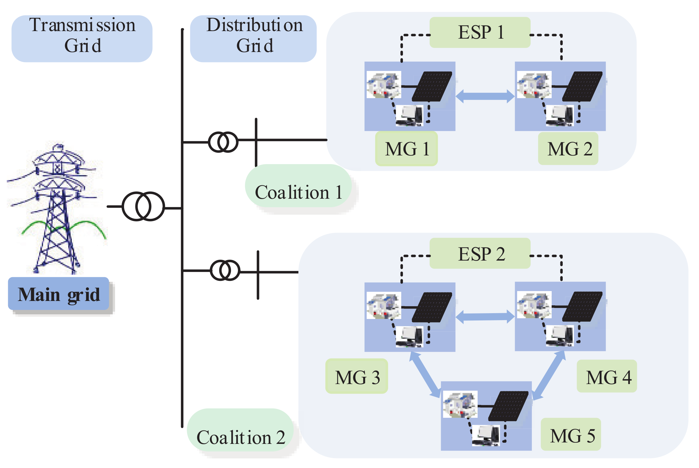
2. Energy Sharing Structure of MGs in Coalition
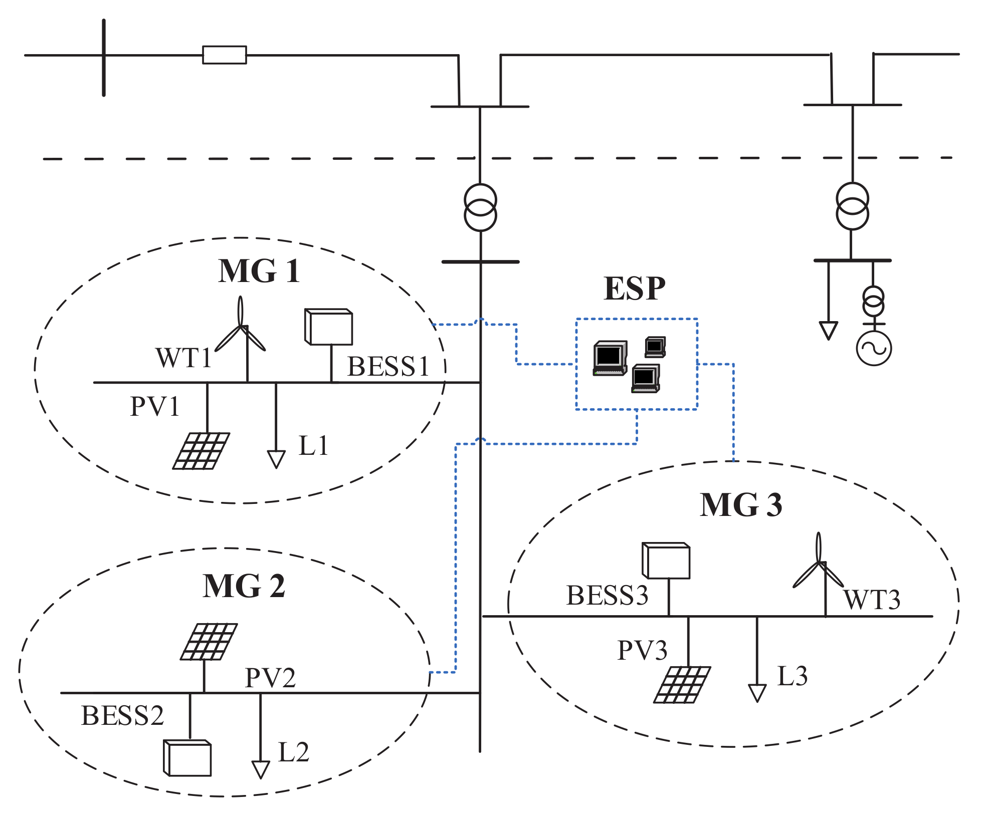
2.1. System Structure
2.2. Energy Sharing Structure of MGs
3. Optimal Dispatching Model of MGs and ESP
3.1. RESs Model
3.2. BESS Model
3.3. Model of CHP System
3.4. Power Loss Model
3.5. Optimal Dispatching Model of MG
3.6. Basic Optimal Dispatching Model of MGs and ESP
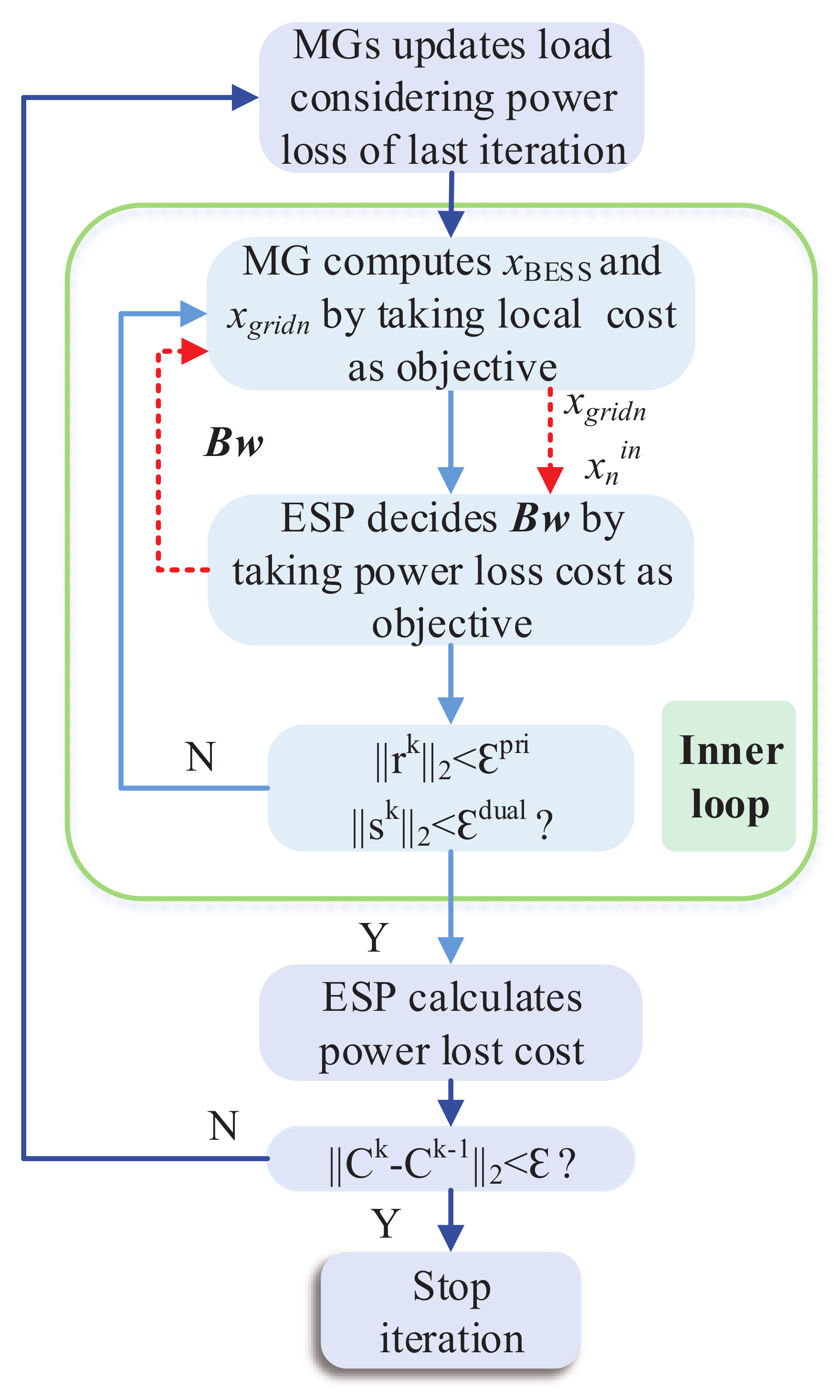
4. Distributed Optimal Dispatching Model and Algorithm of MGs and ESP Based on ADMM
4.1. Distributed Optimal Dispatching Model of MGs and ESP Based on ADMM
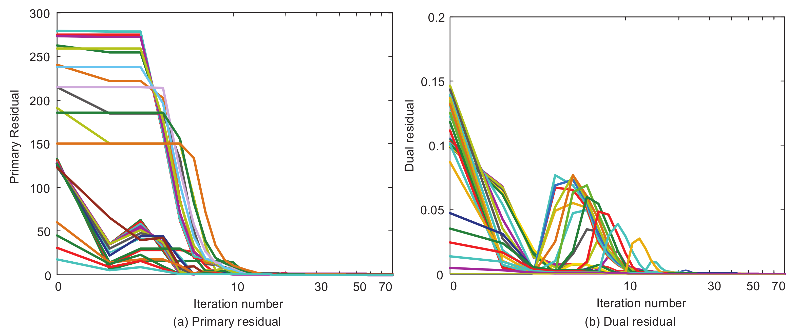
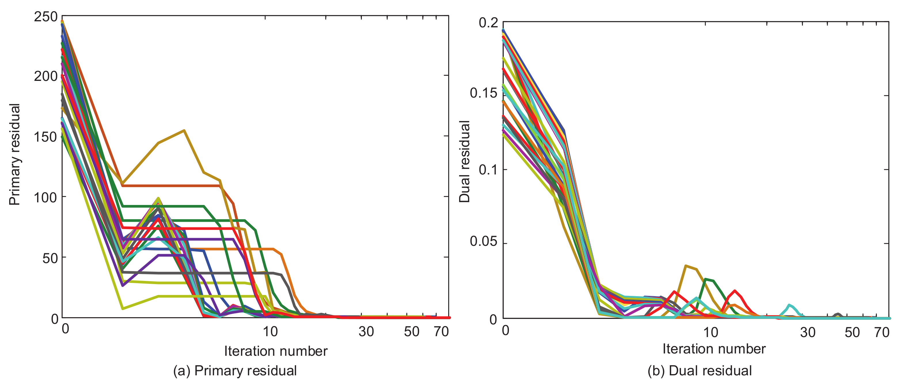
4.2. Convergence Condition and Distributed Optimal Algorithm
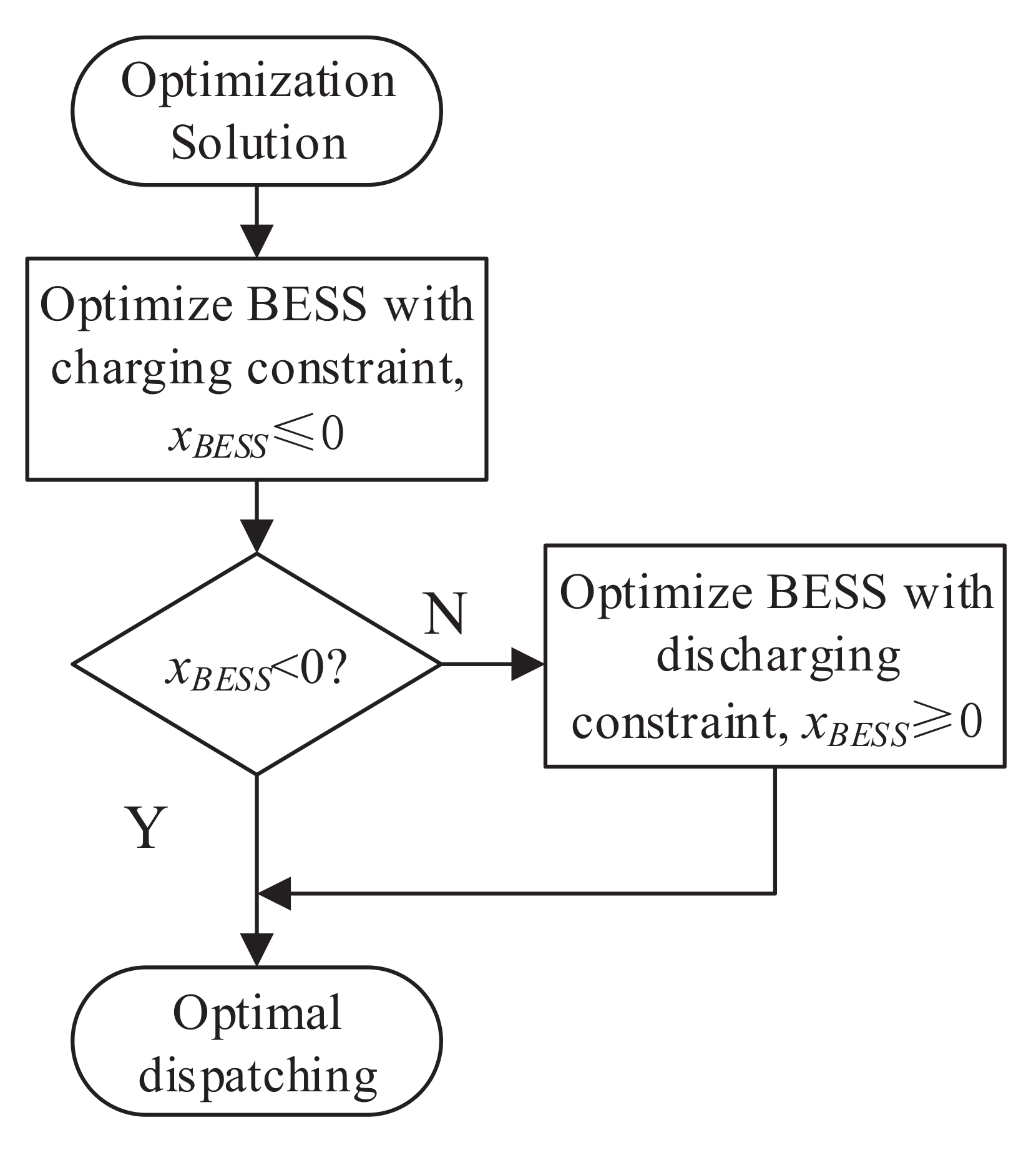
4.3. Optimization Solution of MGs in the Iteration Process
4.4. Distributed Optimal Algorithm
| Algorithm 1 Distributed optimal dispatching algorithm. |
|
5. Case Study
5.1. Scenario 1
5.1.1. Basic Data in Scenario 1
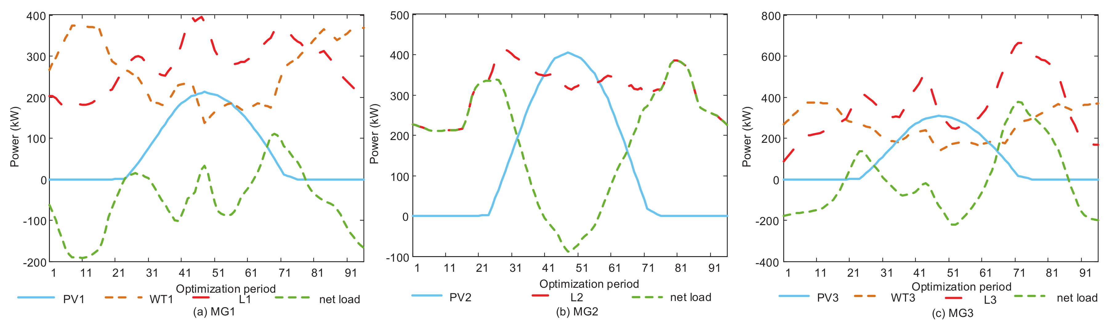
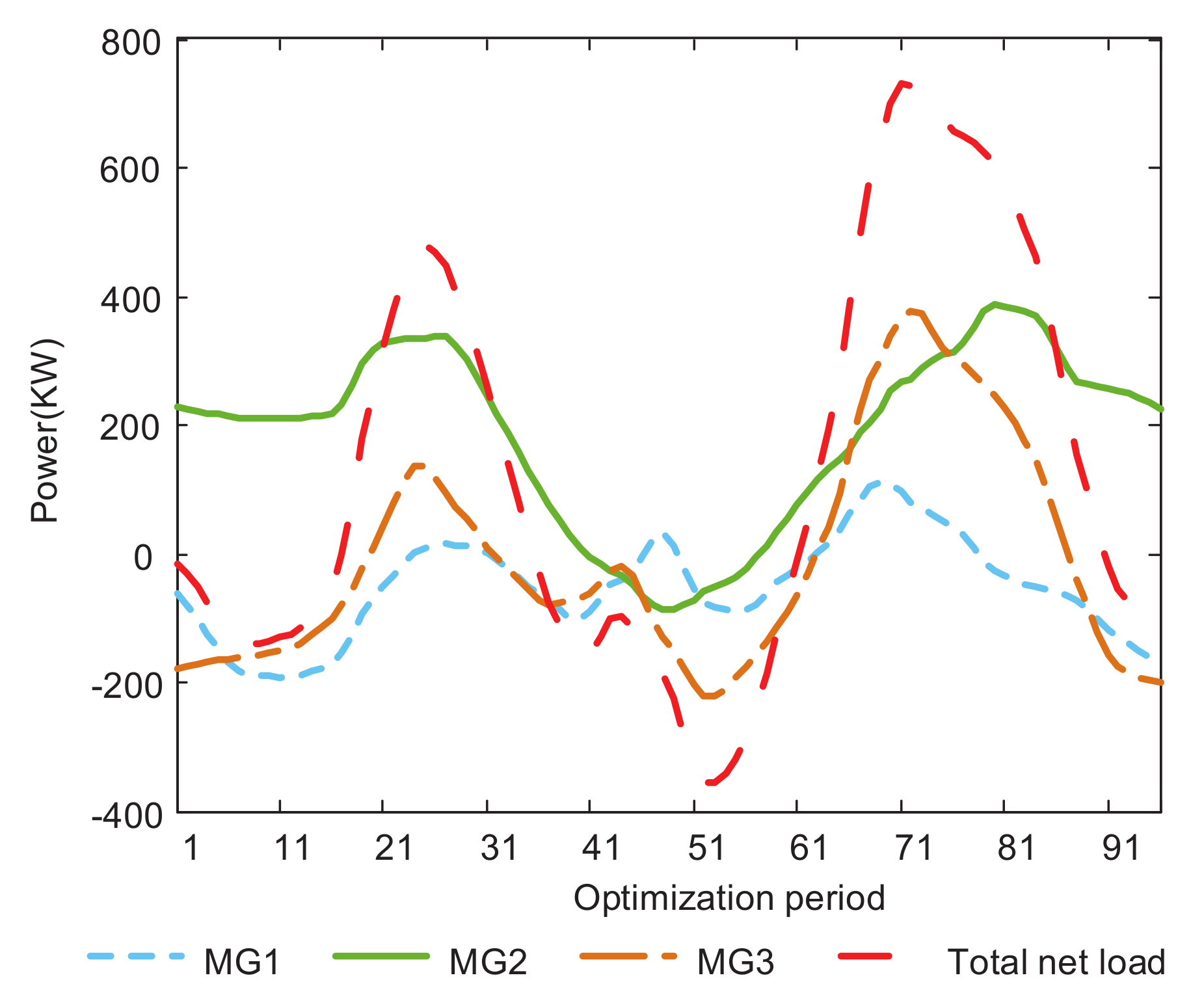
5.1.2. Optimal Results on Different Days for One Week
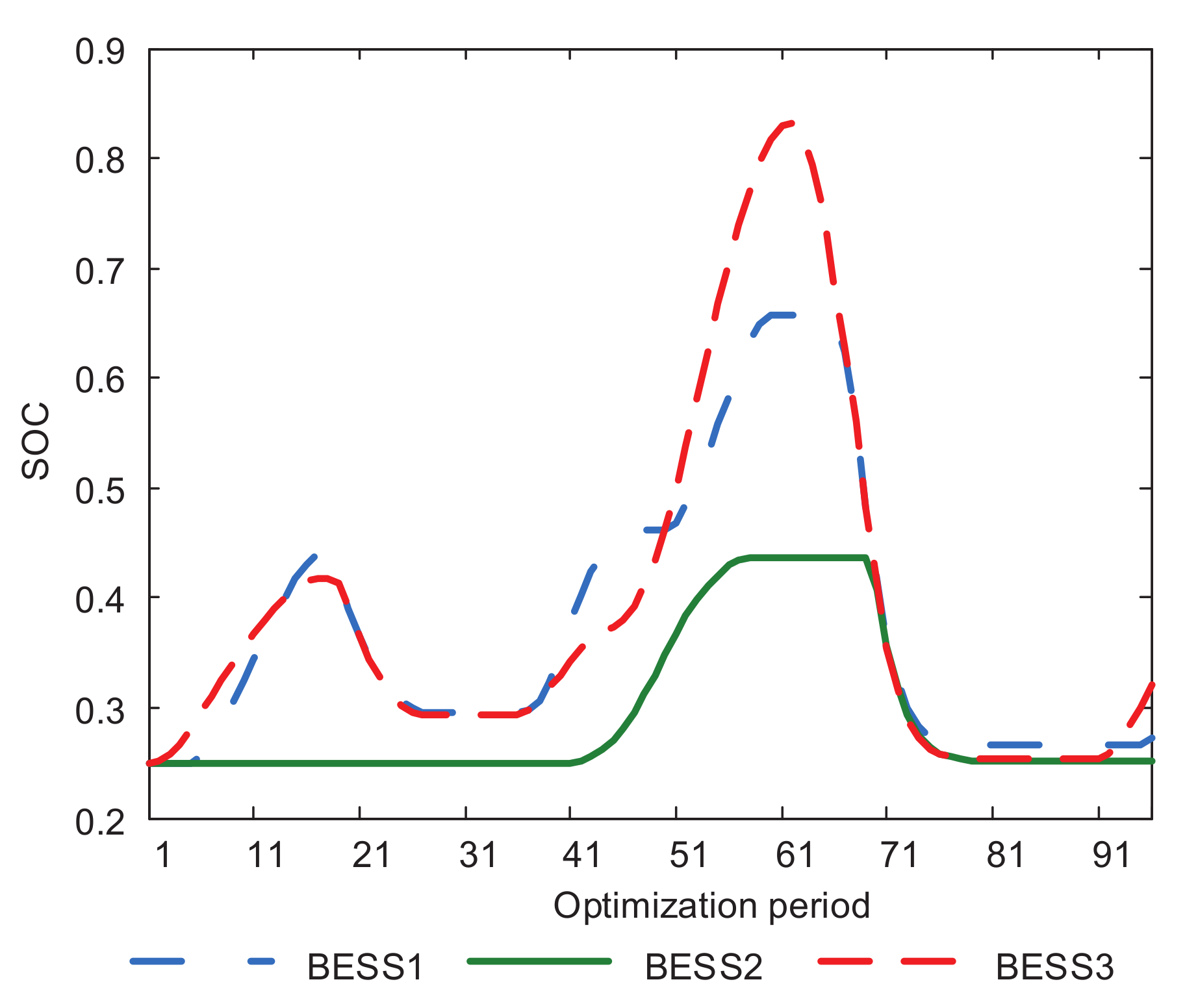
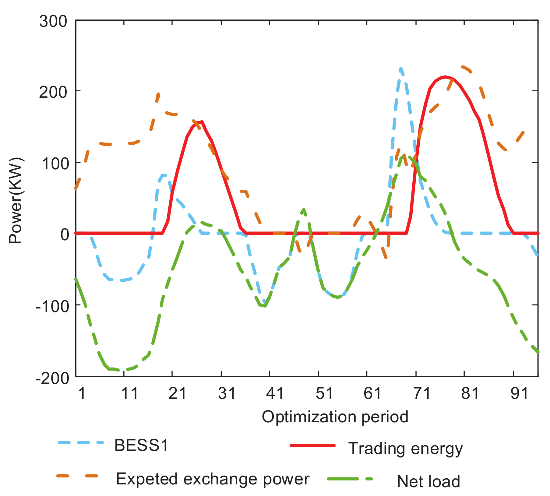
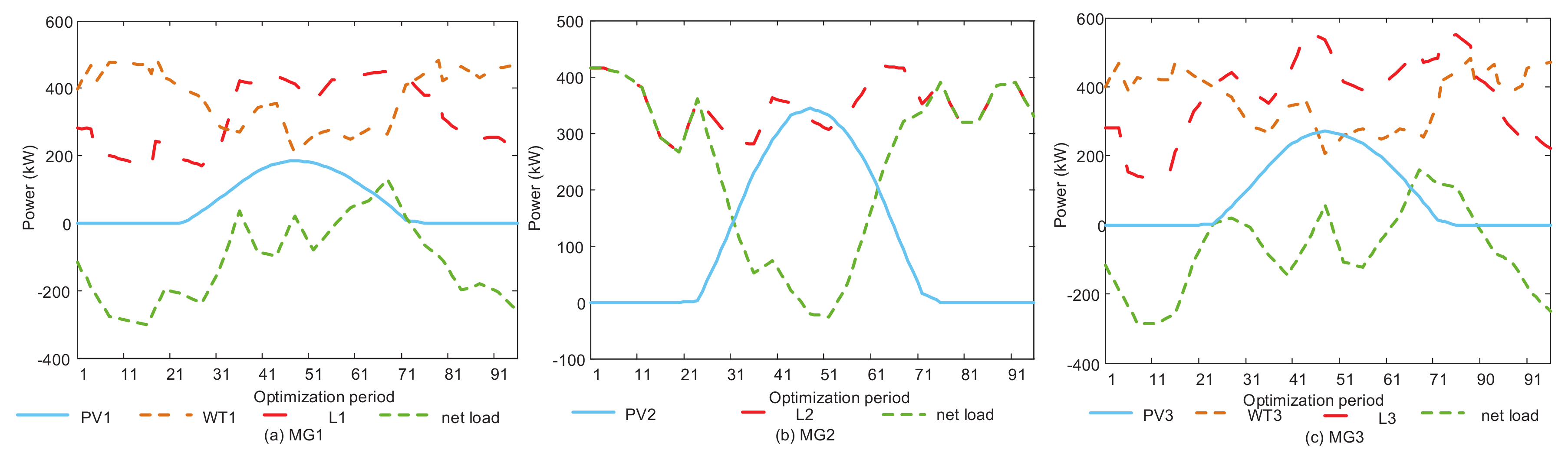
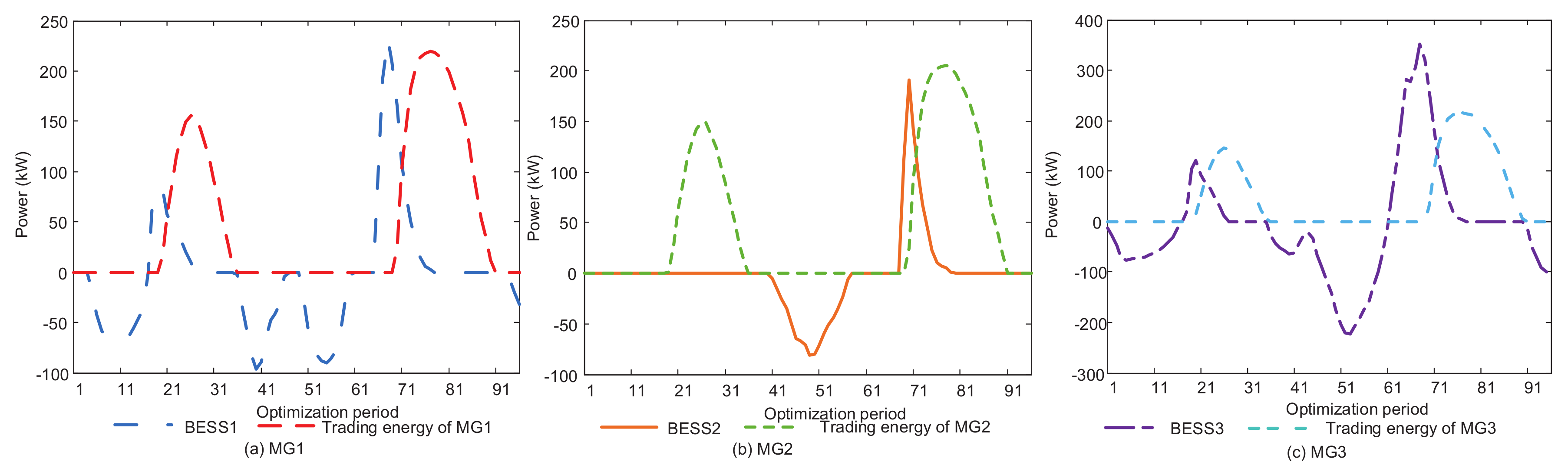
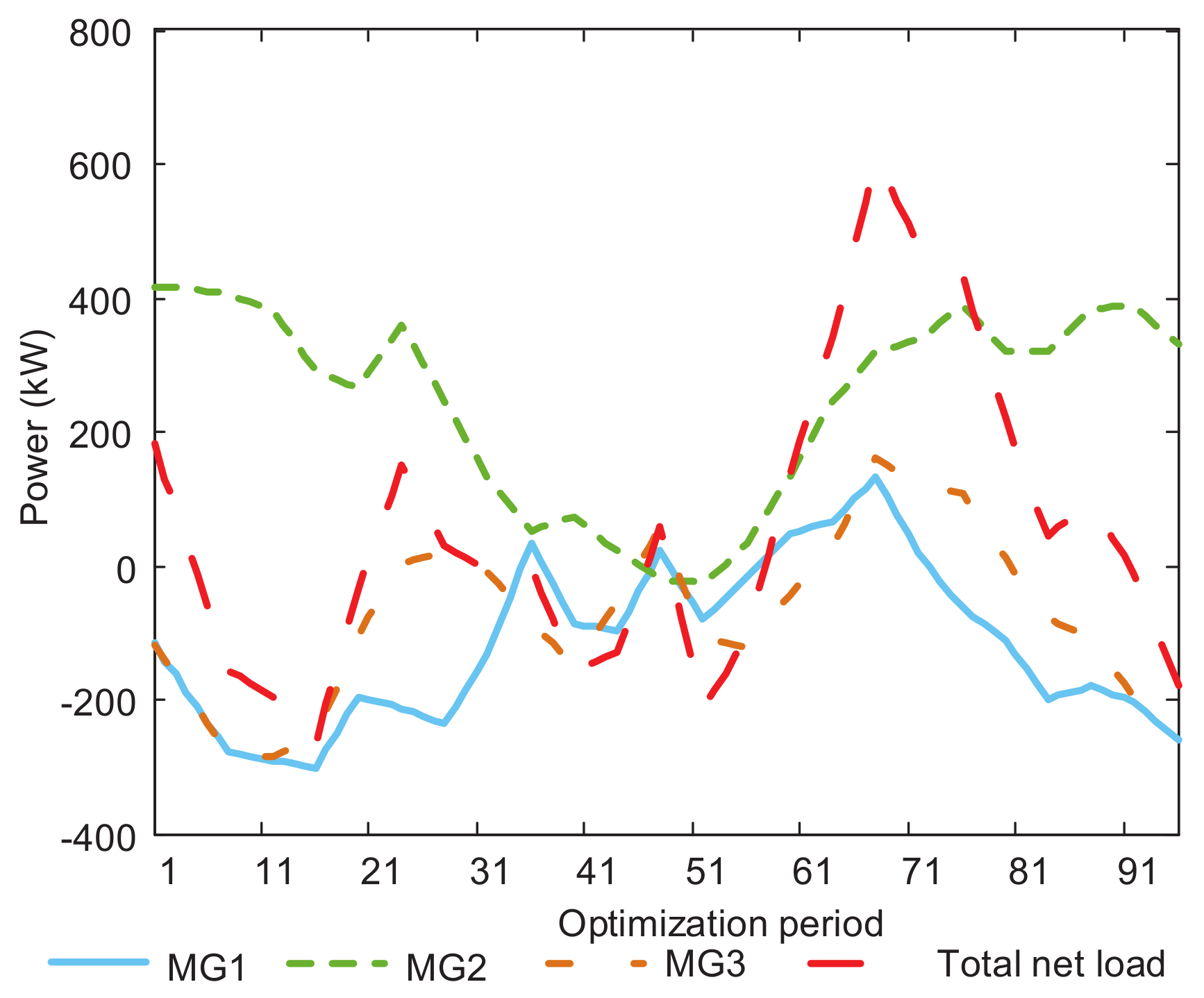
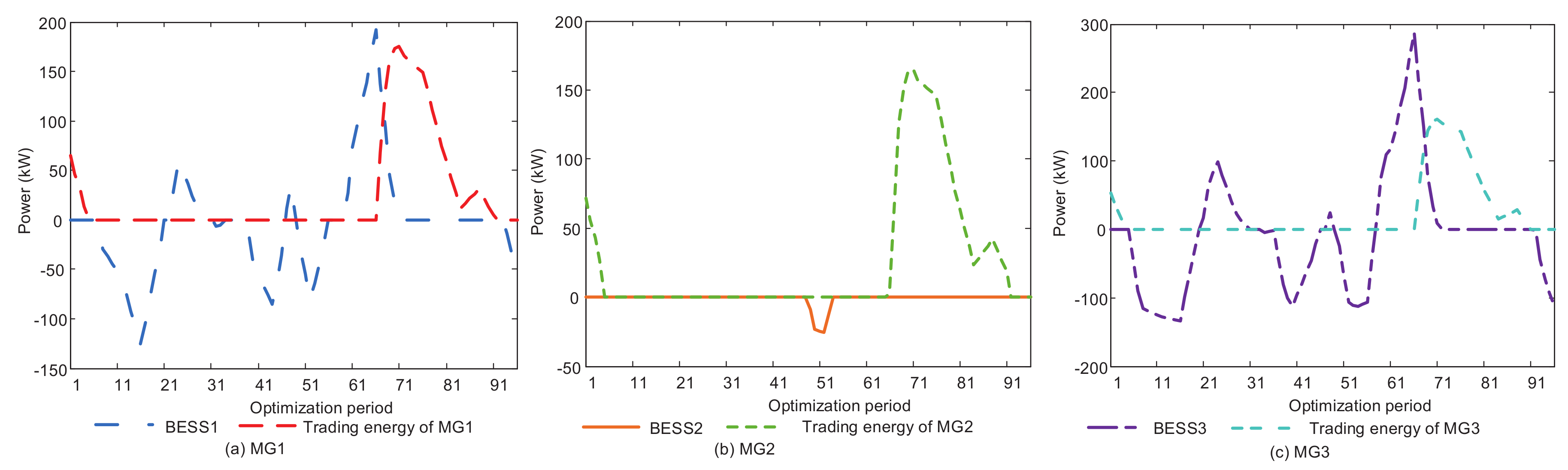
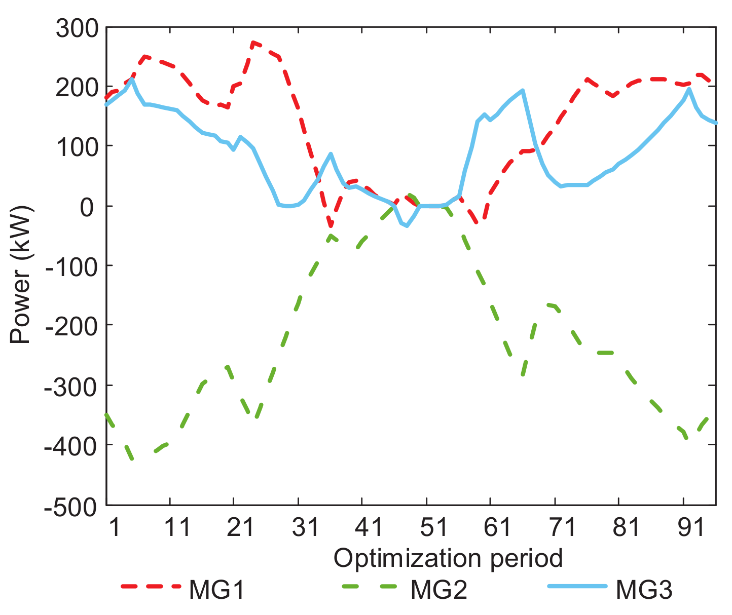
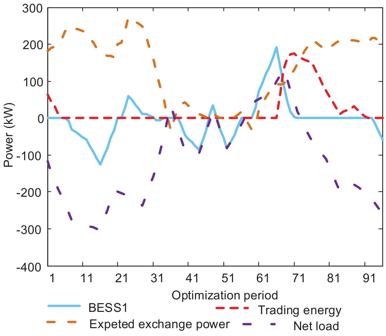
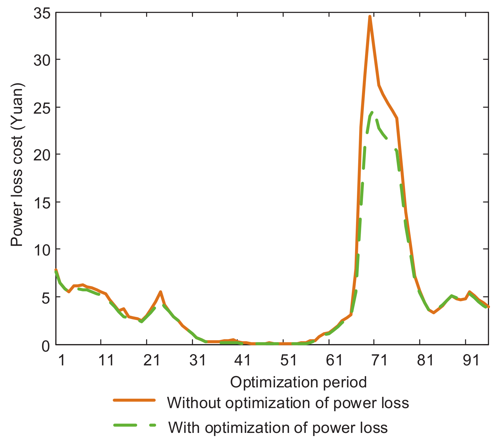
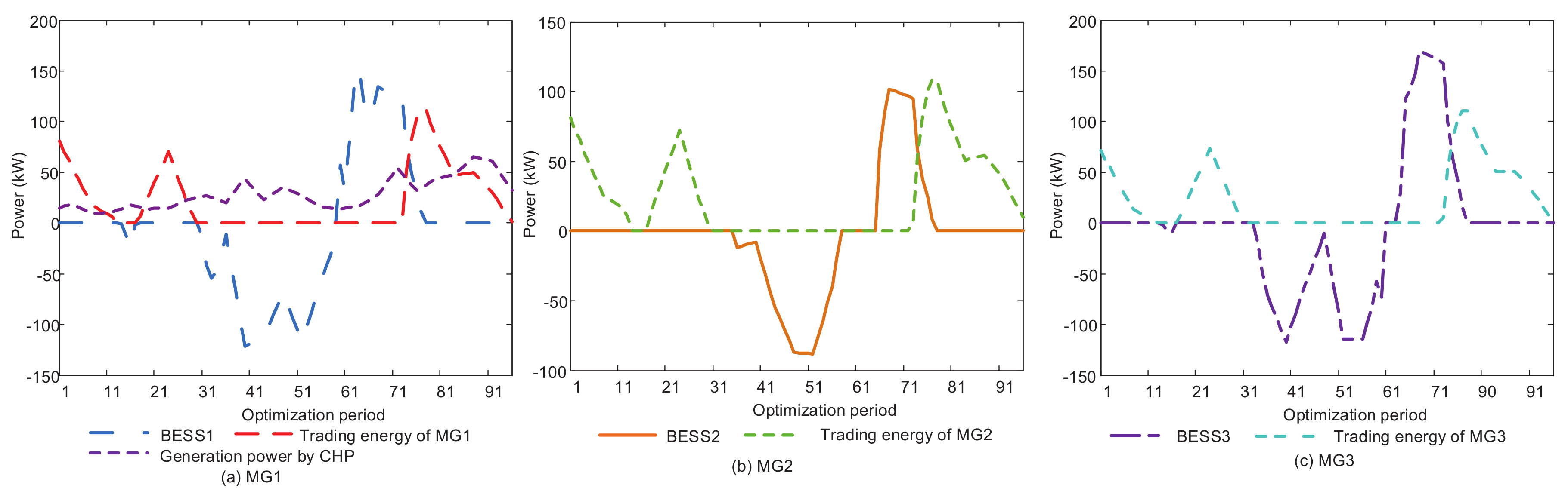
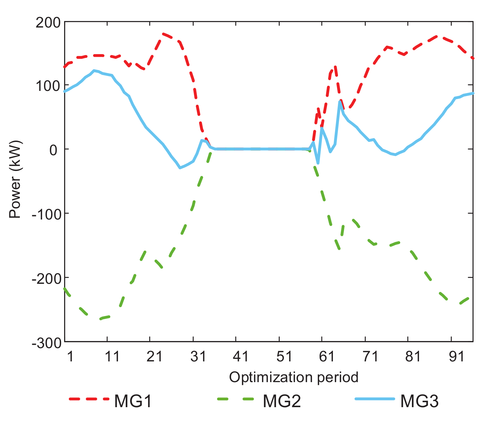
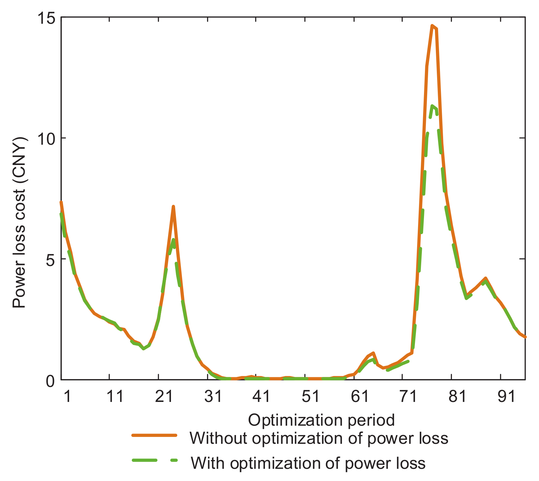
5.1.3. Results and Analysis of the Distributed Optimal Dispatching on Day 1 of Scenario 1
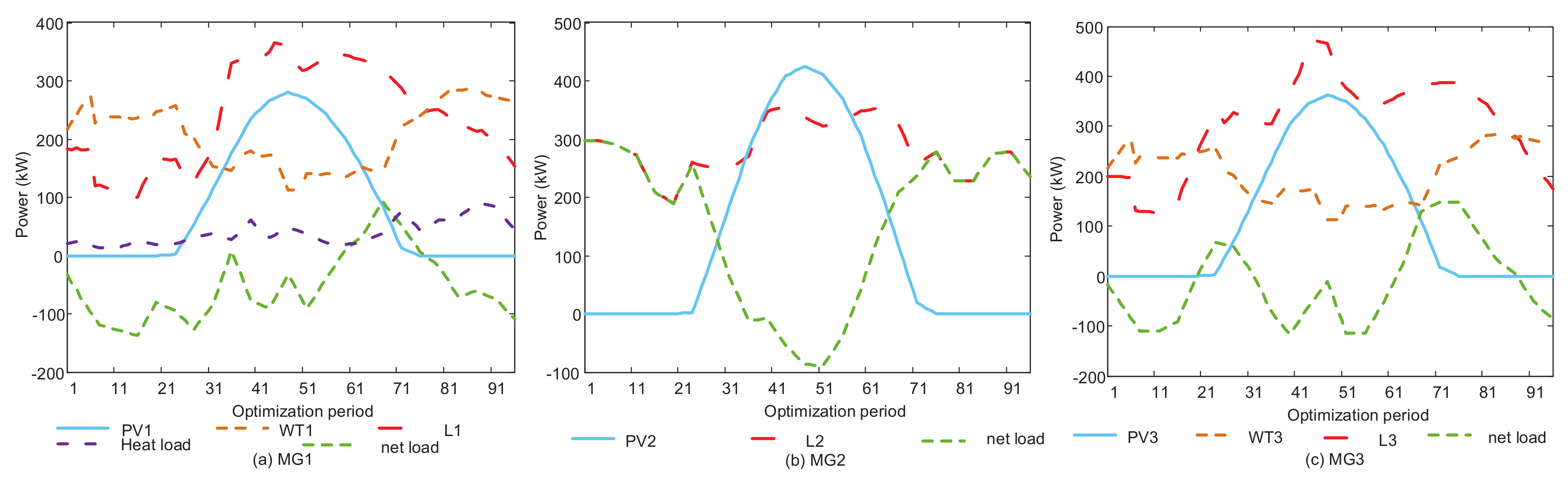
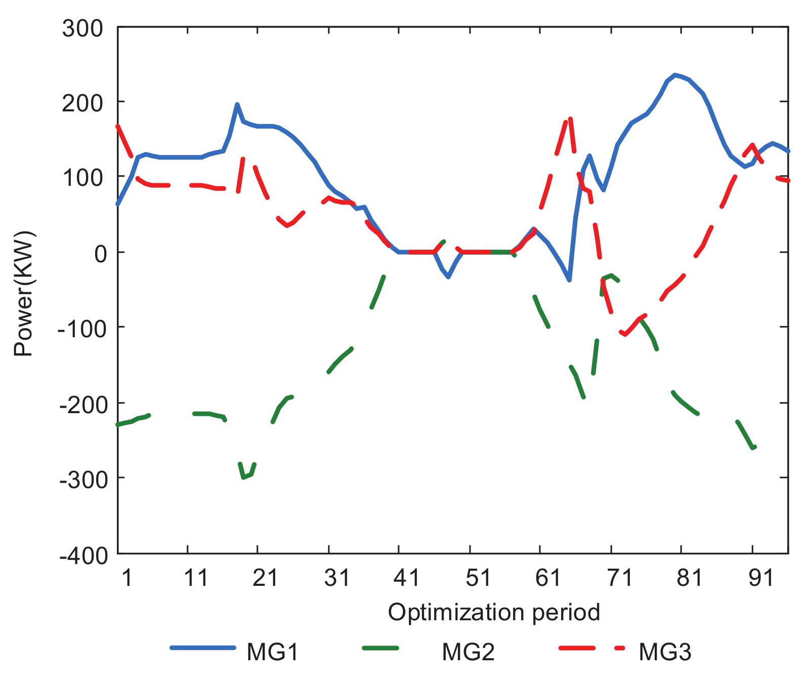
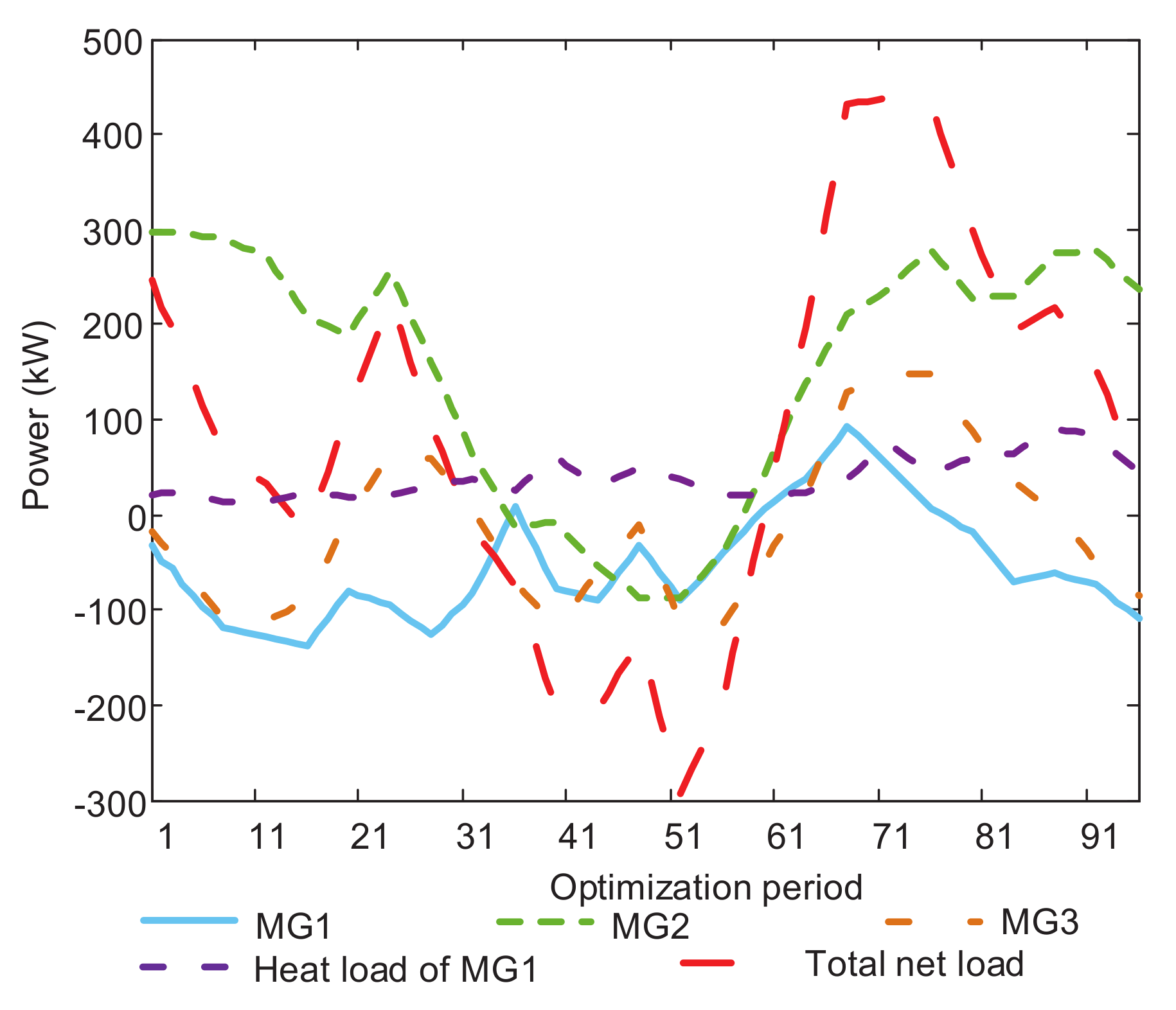
5.1.4. Results and Analysis of the Distributed Optimal Dispatching on Day 2 of Scenario 1
5.2. Scenario 2
5.2.1. Basic Data in Scenario 2
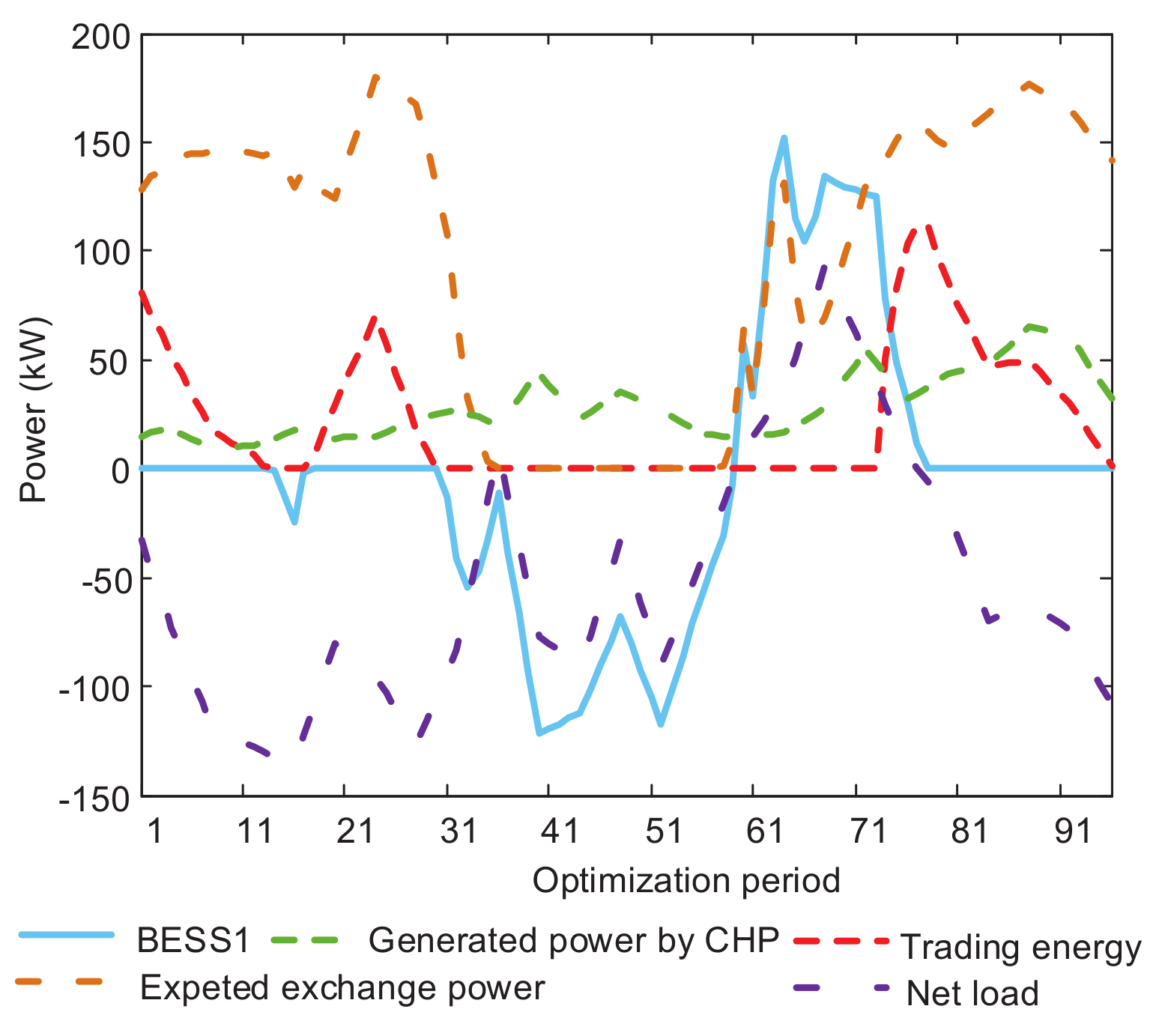
5.2.2. Results and Analysis of the Distributed Optimal Dispatching in Scenario 2
5.3. Comparison with the Related Work
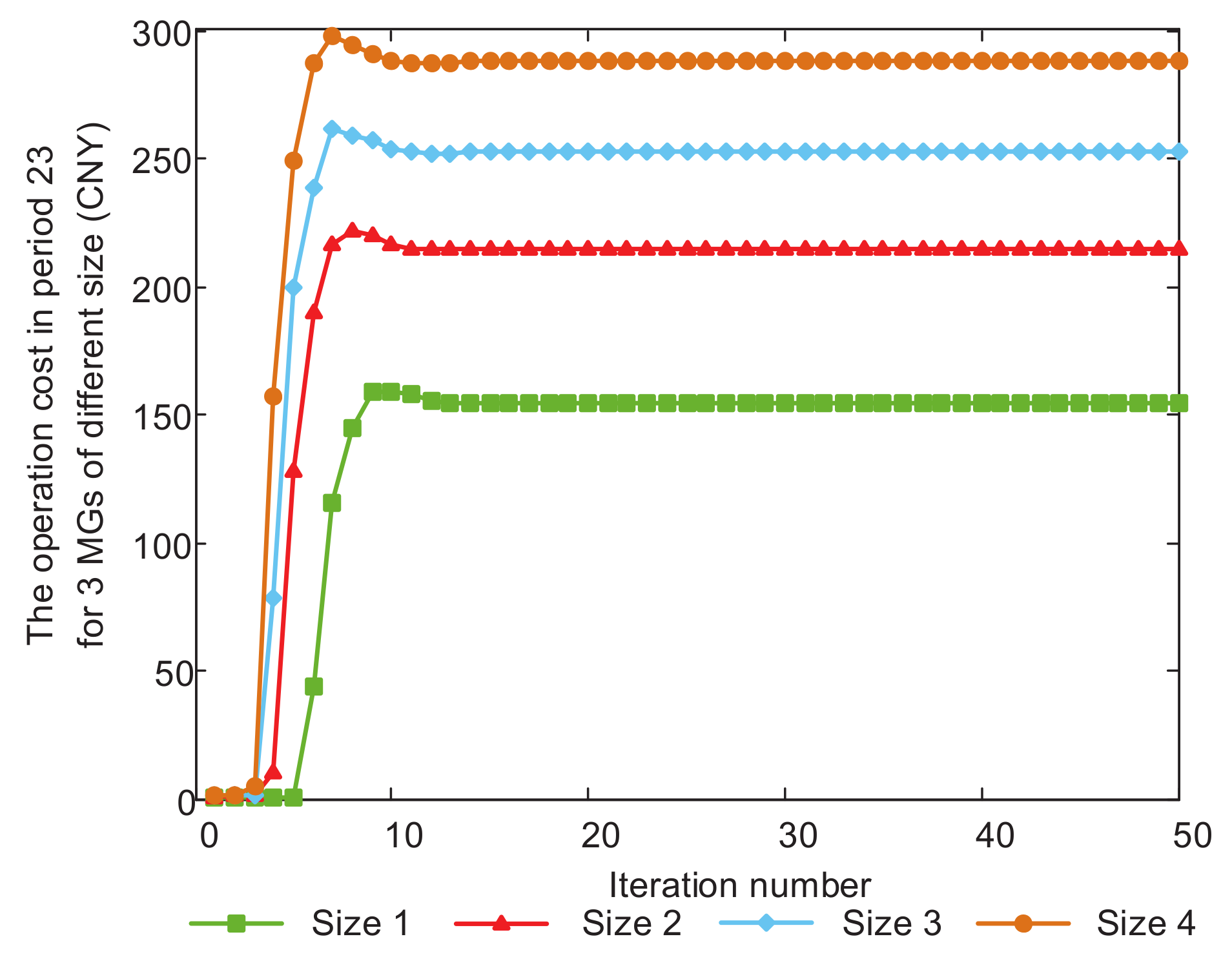
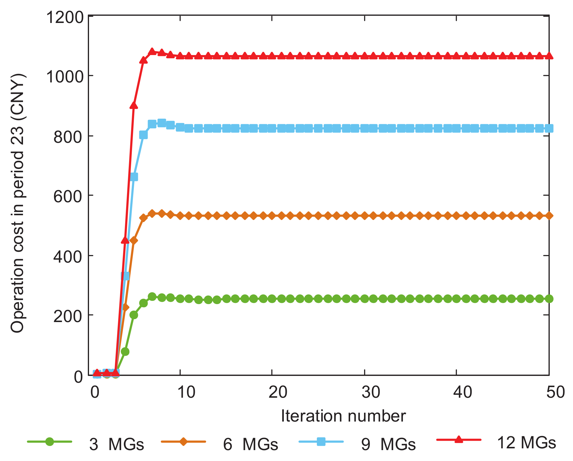
5.4. Scalability Analysis
6. Conclusions
Acknowledgments
Author Contributions
Conflicts of Interest
Nomenclature
| The output power of PV | |
| Light intensity | |
| Maximum test power under the standard testing environment | |
| Light intensity under the standard testing environment | |
| Power temperature coefficient | |
| Temperature of the photovoltaic cell | |
| Reference temperature | |
| The output power of WT | |
| Rated power of WT | |
| a, b, c, d | Fit parameters |
| Cut-in wind speed | |
| Rated wind speed | |
| Cut-out wind speed | |
| The output power of RESs | |
| I | The investment cost of BESS |
| P | The discharging power of BESS |
| The length of the time period | |
| Q | The battery capacity |
| The total cumulative Ah throughput in the life cycle | |
| The initial state of charge | |
| The fuel cost of CHP | |
| The price of natural gas | |
| The electric power of CHP | |
| Low calorific value of natural gas | |
| The heat power of CHP | |
| Heat loss coefficient | |
| Heating coefficient of the LiBr chiller | |
| The total power loss | |
| The power loss over the distributed line between MG n and MG m | |
| Power loss over the distributed line between MG n and the main grid | |
| The resistance of the distribution line between MG n and MG m | |
| The resistance of the distribution line between MG n and the main grid | |
| The total power loss cost | |
| Price per unit of power energy | |
| The charge-discharge power of BESS in MG n | |
| The exchange power between MG n and the main grid | |
| The selling price of the main grid | |
| Load demands of MG n | |
| The exchange power between MG n and other MGs | |
| Charge-discharge efficiency of BESS | |
| , | Maximum and minimum charge-discharge power |
| , | The upper and lower bounds of SOC |
| Penalty parameter | |
| , | The convergence error of the primal residual and dual residual |
References
- Meliopoulos, A.P.S.; Polymeneas, E.; Tan, Z.; Huang, R.; Zhao, D. Advanced Distribution Management System. IEEE Trans. Smart Grid 2013, 4, 2109–2117. [Google Scholar] [CrossRef]
- Kazmi, S.A.A.; Shahzad, M.K.; Khan, A.Z.; Shin, D.R. Smart Distribution Networks: A Review of Modern Distribution Concepts from a Planning Perspective. Energies 2017, 10, 501. [Google Scholar] [CrossRef]
- Zhang, D.; Evangelisti, S.; Lettieri, P.; Papageorgiou, L.G. Optimal design of CHP-based microgrids: Multiobjective optimisation and life cycle assessment. Energy 2015, 85, 181–193. [Google Scholar] [CrossRef]
- Lee, E.K.; Shi, W.; Gadh, R.; Kim, W. Design and Implementation of a Microgrid Energy Management System. Sustainability 2016, 8, 1143. [Google Scholar] [CrossRef]
- Wu, J.; Guan, X. Coordinated Multi-Microgrids Optimal Control Algorithm for Smart Distribution Management System. IEEE Trans. Smart Grid 2013, 4, 2174–2181. [Google Scholar] [CrossRef]
- Liu, N.; Yu, X.; Wang, C.; Wang, J. Energy Sharing Management for Microgrids with PV Prosumers: A Stackelberg Game Approach. IEEE Trans. Ind. Inform. 2017, 13, 1088–1098. [Google Scholar] [CrossRef]
- Tushar, M.H.K.; Assi, C. Optimal Energy Management and Marginal-Cost Electricity Pricing in Microgrid Network. IEEE Trans. Ind. Inform. 2017, 13, 3286–3298. [Google Scholar] [CrossRef]
- Aluisio, B.; Dicorato, M.; Forte, G.; Trovato, M. An optimization procedure for Microgrid day-ahead operation in the presence of CHP facilities. Sustain. Energy Grids Netw. 2017, 11, 34–45. [Google Scholar] [CrossRef]
- Liu, N.; Wang, J.; Wang, L. Distributed energy management for interconnected operation of combined heat and power-based microgrids with demand response. J. Mod. Power Syst. Clean Energy 2017, 5, 1–11. [Google Scholar] [CrossRef]
- Zhou, X.; Ai, Q.; Wang, H. Adaptive Marginal Costs-Based Distributed Economic Control of Microgrid Clusters Considering Line Loss. Energies 2017, 10, 2071. [Google Scholar] [CrossRef]
- Liu, Y.; Fang, Y.; Li, J. Interconnecting Microgrids via the Energy Router with Smart Energy Management. Energies 2017, 10, 1297. [Google Scholar] [CrossRef]
- Liu, N.; Yu, X.; Wang, C.; Li, C.; Ma, L.; Lei, J. Energy-Sharing Model with Price-Based Demand Response for Microgrids of Peer-to-Peer Prosumers. IEEE Trans. Power Syst. 2017, 32, 3569–3583. [Google Scholar] [CrossRef]
- Ma, L.; Liu, N.; Zhang, J.; Tushar, W.; Yuen, C. Energy Management for Joint Operation of CHP and PV Prosumers Inside a Grid-Connected Microgrid: A Game Theoretic Approach. IEEE Trans. Ind. Inform. 2016, 12, 1930–1942. [Google Scholar] [CrossRef]
- Wang, J.; Zhong, H.; Xia, Q.; Kang, C.; Du, E. Optimal joint-dispatch of energy and reserve for CCHP-based microgrids. IET Gener. Transm. Distrib. 2017, 11, 785–794. [Google Scholar] [CrossRef]
- Liu, N.; He, L.; Yu, X.; Ma, L. Multi-Party Energy Management for Grid-Connected Microgrids with Heat and Electricity Coupled Demand Response. IEEE Trans. Ind. Inform. 2017. [Google Scholar] [CrossRef]
- Shao, C.; Ding, Y.; Wang, J.; Song, Y. Modeling and Integration of Flexible Demand in Heat and Electricity Integrated Energy System. IEEE Trans. Sustain. Energy 2017, 9, 361–370. [Google Scholar] [CrossRef]
- Jang, Y.S.; Kim, M.K. A Dynamic Economic Dispatch Model for Uncertain Power Demands in an Interconnected Microgrid. Energies 2017, 10, 300. [Google Scholar] [CrossRef]
- Gregoratti, D.; Matamoros, J. Distributed Energy Trading: The Multiple-Microgrid Case. IEEE Trans. Ind. Electron. 2014, 62, 2551–2559. [Google Scholar] [CrossRef]
- Zhang, C.; Zhang, Y.J. Optimal distributed generation placement among interconnected cooperative microgrids. In Proceedings of the Power and Energy Society General Meeting, Boston, MA, USA, 17–21 July 2016; pp. 1–5. [Google Scholar]
- Minciardi, R.; Robba, M. A Bilevel Approach for the Stochastic Optimal Operation of Interconnected Microgrids. IEEE Trans. Autom. Sci. Eng. 2016, 14, 482–493. [Google Scholar] [CrossRef]
- Che, L.; Zhang, X.; Shahidehpour, M.; Alabdulwahab, A.; Abusorrah, A. Optimal Interconnection Planning of Community Microgrids with Renewable Energy Sources. IEEE Trans. Smart Grid 2017, 8, 1054–1063. [Google Scholar] [CrossRef]
- Mbuwir, B.; Ruelens, F.; Spiessens, F.; Deconinck, G. Battery Energy Management in a Microgrid Using Batch Reinforcement Learning. Energies 2017, 10, 1846. [Google Scholar] [CrossRef]
- Jia, K.; Chen, Y.; Bi, T.; Lin, Y.; Thomas, D.; Sumner, M. Historical data based energy management in a micro-grid with a hybrid energy storage system. IEEE Trans. Ind. Inform. 2017, 13, 2597–2605. [Google Scholar] [CrossRef]
- Liu, N.; Wang, C.; Cheng, M.; Wang, J. A Privacy-Preserving Distributed Optimal Scheduling for Interconnected Microgrids. Energies 2016, 9, 1031. [Google Scholar] [CrossRef]
- Chiu, W.Y.; Sun, H.; Poor, H.V. A Multiobjective Approach to Multimicrogrid System Design. IEEE Trans. Smart Grid 2017, 6, 2263–2272. [Google Scholar] [CrossRef]
- Tu, A.N.; Crow, M.L. Stochastic Optimization of Renewable-Based Microgrid Operation Incorporating Battery Operating Cost. IEEE Trans. Power Syst. 2016, 31, 2289–2296. [Google Scholar]
- Arefifar, S.A.; Ordonez, M.; Mohamed, A.R.I. Energy Management in Multi-Microgrid Systems—Development and Assessment. IEEE Trans. Power Syst. 2017, 32, 910–922. [Google Scholar]
- Liu, Y.; Li, Y.; Gooi, H.B.; Ye, J.; Xin, H.; Jiang, X.; Pan, J. Distributed Robust Energy Management of a Multi-Microgrid System in the Real-Time Energy Market. IEEE Trans. Sustain. Energy 2017. [Google Scholar] [CrossRef]
- Liu, N.; Chen, Q.; Liu, J.; Lu, X.; Li, P.; Lei, J.; Zhang, J. A Heuristic Operation Strategy for Commercial Building Microgrids Containing EVs and PV System. IEEE Trans. Ind. Electron. 2015, 62, 2560–2570. [Google Scholar] [CrossRef]
- Hong, Y.Y.; Yo, P.S. Novel Genetic Algorithm-Based Energy Management in a Factory Power System Considering Uncertain Photovoltaic Energies. Appl. Sci. 2017, 7, 438. [Google Scholar] [CrossRef]
- Liu, Z.; Chen, Y.; Luo, Y.; Zhao, G.; Jin, X. Optimized Planning of Power Source Capacity in Microgrid, Considering Combinations of Energy Storage Devices. Appl. Sci. 2016, 6, 416. [Google Scholar] [CrossRef]
- Bansal, M.; Dhillon, J. Market bid optimization of a hybrid solar-wind system using CAES. In Proceedings of the India International Conference on Power Electronics, Patiala, India, 17–19 November 2016; pp. 1–4. [Google Scholar]
- Chedid, R.; Akiki, H.; Rahman, S. A decision support technique for the design of hybrid solar-wind power systems. IEEE Trans. Energy Convers. 2002, 13, 76–83. [Google Scholar] [CrossRef]
- Deng, Q.; Gao, X.; Zhou, H.; Hu, W. System modeling and optimization of microgrid using genetic algorithm. In Proceedings of the International Conference on Intelligent Control and Information Processing, Harbin, China, 25–28 July 2011; pp. 540–544. [Google Scholar]
- Shi, W.; Xie, X.; Chu, C.C.; Gadh, R. Distributed Optimal Energy Management in Microgrids. IEEE Trans. Smart Grid 2015, 6, 1137–1146. [Google Scholar] [CrossRef]
- Zhao, B.; Zhang, X.; Chen, J.; Wang, C.; Guo, L. Operation optimization of standalone microgrids considering lifetime characteristics of battery energy storage system. IEEE Trans. Sustain. Energy 2013, 4, 934–943. [Google Scholar] [CrossRef]
- Saad, W.; Han, Z.; Poor, H.V. Coalitional Game Theory for Cooperative Micro-Grid Distribution Networks. In Proceedings of the 2011 IEEE International Conference on Communications Workshops (ICC), Kyoto, Japan, 5–9 June 2011; pp. 1–5. [Google Scholar]
- Fathi, M.; Bevrani, H. Statistical Cooperative Power Dispatching in Interconnected Microgrids. IEEE Trans. Sustain. Energy 2013, 4, 586–593. [Google Scholar] [CrossRef]
- Matamoros, J.; Gregoratti, D.; Dohler, M. Microgrids energy trading in islanding mode. In Proceedings of the 2012 IEEE Third International Conference on Smart Grid Communications (SmartGridComm), Tainan, Taiwan, 5–8 November 2012; pp. 49–54. [Google Scholar]
- Boyd, S.; Parikh, N.; Chu, E.; Peleato, B.; Eckstein, J. Distributed Optimization and Statistical Learning via the Alternating Direction Method of Multipliers. Found. Trends Mach. Learn. 2010, 3, 1–122. [Google Scholar] [CrossRef]
- Liu, N.; Tang, Q.; Zhang, J.; Fan, W.; Liu, J. A hybrid forecasting model with parameter optimization for short-term load forecasting of micro-grids. Appl. Energy 2014, 129, 336–345. [Google Scholar] [CrossRef]
- Li, Y.; Liu, N.; Zhang, J. Jointly optimization and distributed control for interconnected operation of autonomous microgrids. In Proceedings of the Innovative Smart Grid Technologies—Asia, Bangkok, Thailand, 3–6 November 2016; pp. 1–6. [Google Scholar]


| RES | Rated Capacity (kW) |
|---|---|
| WT1 | 500 |
| PV1 | 500 |
| PV2 | 800 |
| WT3 | 500 |
| PV3 | 800 |
| BESS | Rated Power (kW) | Rated Capacity (kWh) | I (Yuan) |
|---|---|---|---|
| BESS1 | 250 | 800 | 800,000 |
| BESS2 | 350 | 1000 | 1,000,000 |
| BESS3 | 400 | 1200 | 1,200,000 |
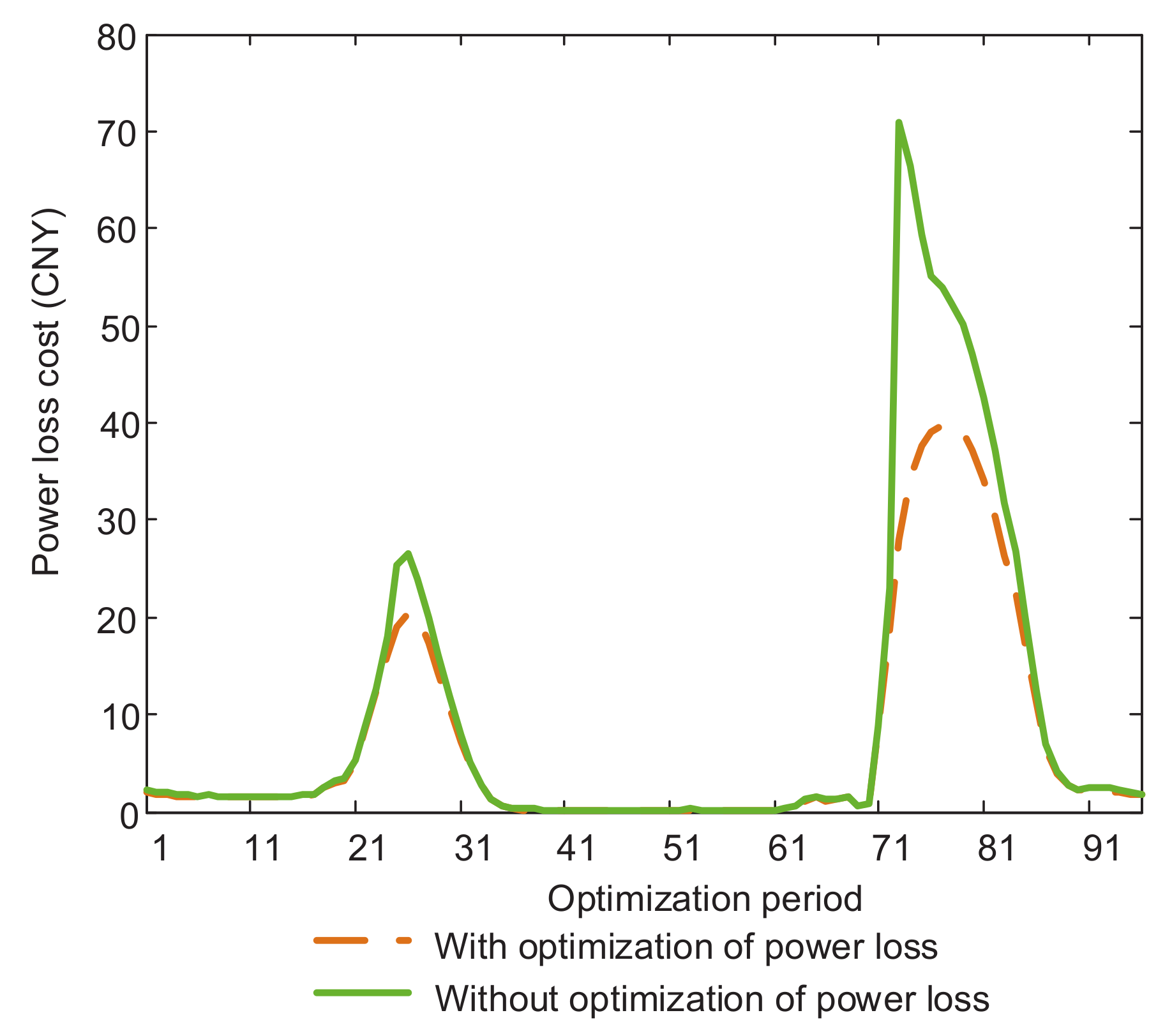
| Days | Total Operation Cost (CNY) | Power Loss Cost without Optimization of Power Loss (CNY) | Power Loss Cost with Optimization of Power Loss (CNY) | Average Iteration Number |
|---|---|---|---|---|
| Day 1 | 10,449.7 | 900.7 | 697.5 | 33 |
| Day 2 | 5777.4 | 483.9 | 457.9 | 37 |
| Day 3 | 8991.1 | 807.9 | 675.1 | 37 |
| Day 4 | 10,373.1 | 734.2 | 636.2 | 29 |
| Day 5 | 6429.2 | 513.9 | 453.8 | 37 |
| Day 6 | 13,606.4 | 1431.4 | 1063.3 | 30 |
| Day 7 | 11,120.8 | 821.6 | 676.9 | 32 |
| RES | Rated Capacity (kW) |
|---|---|
| WT1 | 400 |
| PV1 | 400 |
| PV2 | 600 |
| WT3 | 400 |
| PV3 | 500 |
| BESS | Rated Power (kW) | Rated Capacity (kWh) | I (Yuan) |
|---|---|---|---|
| BESS1 | 250 | 800 | 800,000 |
| BESS2 | 200 | 600 | 600,000 |
| BESS3 | 350 | 1000 | 1,000,000 |
| Parameter Name | Parameter Value |
|---|---|
| Rated electrical power | 500 kW |
| 0.35 | |
| 1.5 CNY/kWh | |
| 0.05 | |
| 0.8 |
| Cost | With Optimization | Without Optimization |
|---|---|---|
| Power loss cost (CNY) | 207.92 | 230.98 |
| Properties | Ref. [42] | Ref. [18] | Ref. [38] | This Paper |
|---|---|---|---|---|
| RESs | - | - | PV | PV WT |
| Optimize power loss? | No | No | No | Yes |
| Optimize BESS? | No | No | No | Yes |
| Operation mode of MGs | Island mode | Island mode | Grid-connected | Grid-connected |
| Exchanged information | All data of sources and load transmitted to control center | Price and expected purchasing energy quantities | Price and expected purchasing energy quantities | Expected exchange power |
| Solution algorithm | Centralized optimization | Based on subgradient | statistical cooperative power dispatching (SCPD) algorithm | Based on alternating direction method of multipliers (ADMM). |
| Iteration number | - | About 100 | 93 | Average 33.33 |
| The Number of MGs | Total Operation Cost (CNY) | Average Iteration Number |
|---|---|---|
| 3 MGs | 10,449.7 | 33.33 |
| 6 MGs | 22,905.7 | 33.50 |
| 9 MGs | 34,716.3 | 36.04 |
| 12 MGs | 46,045.1 | 37.32 |
| Sizes | Total Operation Cost (CNY) |
|---|---|
| Size 1 | 6379.0 |
| Size 2 | 8760.7 |
| Size 3 | 10,449.7 |
| Size 4 | 11,580.5 |
© 2018 by the authors. Licensee MDPI, Basel, Switzerland. This article is an open access article distributed under the terms and conditions of the Creative Commons Attribution (CC BY) license (http://creativecommons.org/licenses/by/4.0/).
Share and Cite
Liu, N.; Wang, J. Energy Sharing for Interconnected Microgrids with a Battery Storage System and Renewable Energy Sources Based on the Alternating Direction Method of Multipliers. Appl. Sci. 2018, 8, 590. https://doi.org/10.3390/app8040590
Liu N, Wang J. Energy Sharing for Interconnected Microgrids with a Battery Storage System and Renewable Energy Sources Based on the Alternating Direction Method of Multipliers. Applied Sciences. 2018; 8(4):590. https://doi.org/10.3390/app8040590
Chicago/Turabian StyleLiu, Nian, and Jie Wang. 2018. "Energy Sharing for Interconnected Microgrids with a Battery Storage System and Renewable Energy Sources Based on the Alternating Direction Method of Multipliers" Applied Sciences 8, no. 4: 590. https://doi.org/10.3390/app8040590
APA StyleLiu, N., & Wang, J. (2018). Energy Sharing for Interconnected Microgrids with a Battery Storage System and Renewable Energy Sources Based on the Alternating Direction Method of Multipliers. Applied Sciences, 8(4), 590. https://doi.org/10.3390/app8040590