Abstract
It is attractive to extract and determine the key features of traffic patterns for mitigating road congestion and predicting travel time of vehicles in traffic analysis. Based on the previous work that is a scalable approach via a Hadoop MapReduce programming model, this paper aims to extract significant patterns of travel time intervals of vehicles from freeway traffic in Taiwan, and meanwhile to compute the statistics of these patterns from the point of view one may concern. Experimental resources are the records of timestamp gantry sequences of vehicles passed in five months from 2016/11 to 2017/3 that were downloaded from the Traffic Data Collection System, one of Taiwan government open data platforms. To select one specific gantry sequence for demonstration, the longest sequence on the trip within the Taiwan National Freeway No. 5 is selected. Experimental results show that some statistics of vehicle travel time intervals according to 24 h per day are computed for illustration. These statistics can not only provide clues to experts to analyze traffic congestions, but also help drivers how to avoid rush hours. Furthermore, this work is able to handle a larger amount of real data and be promising for further traffic and transportation research in the future.
1. Introduction
In classical static analysis, the sensitivity information of link travel cost mainly holds the decision-making of considering new road links to be added into a transportation network [1,2,3,4]. Currently, the era of big traffic data, huge historic and real-time traffic data is well generated from the so-called Intelligent Transportation Systems (ITS) such that data-driven methods are widely applied to traffic analysis and forecast [5]. It is believed that the ability to predict traffic information based on big open data is one of important building blocks to enrich the effectiveness of dynamic traffic control strategies. However, existing studies rely heavily on macroscopic and aggregate viewpoints of traffic data patterns.
In this paper, the authors proposes a microscopic approach [6], which is based on temporal-spatial recording of vehicle passage along a trip on the freeway, to extract some key traffic patterns by using a newly developed method [7]. The amount of the timestamp gantry sequences collected in freeway automatically is very large, and, therefore, it is necessary to have a scalable approach to make the extract of significant temporal patterns practical and possible. The method to extract the significant temporal patterns and their corresponding class frequency distribution of these patterns is adapted from the previous works [7] that had been applied for an U.S.A. patent application as “Wang, Ching-Tu. Method for Extracting Maximal Repeat Patterns and Computing Frequency Distribution Tables. Patent Application Serial Number 15/208,994. 13 July 2016.”
In this study, a significant pattern is defined as one maximal repeat [8] extracted from the gantry timestamp sequences that can not be the subsequences of another pattern all the time. This process of extracting significant travel time patterns is based on the previous work [7] that was a scalable approach via Hadoop MapReduce programming model [9]. There are two passes to extract maximal repeats. The first pass is to verify the right and left boundary of candidate maximal repeats and the second pass is to estimate one candidate maximal repeat as a maximal repeat if that repeat passes both left and right boundary verification. In [10], Wang adopted an external memory approach using only one general computer with limited memory. However, the computational time was too long to be satisfied as a reasonable time, e.g., several weeks, from the practical point of view. In [7], Wang used Hadoop, a distributed computing platform, to speed up that computation. Note that the Hadoop MapReduce programming model is well known for its scalability in solving big data problems [11,12,13].
To show briefly the concept of this study, Figure 1, Figure 2 and Figure 3 are given and described in the following. First of all, Figure 1 shows the passages of five vehicles from left to right on a freeway with their origin and destination interchanges. In particular, a detection gantry, denoted as GID in Figure 1, is located at the mainline section between two adjacent interchanges to capture complete passage of vehicles. Figure 2 gives the corresponding gantry sequences with timestamps according to their trip, respectively. Namely, a timestamp is recorded with one gantry simultaneously when a vehicle is passing that gantry. To show the situation of these five vehicles passing, for simplicity, their timestamps attached with the same gantry are assumed to be the same in Figure 2. That is, the amount of the flow of vehicles passing consecutive gantries can be obtained by computing the frequency of gantry sequences whose corresponding timestamps passing each of these gantries are the same. Figure 3, for example, gives the significant travel time patterns extracted according to those gantry sequences in Figure 2. Note that the pattern “GID_2 GID_3” with specific timestamps is not generated in Figure 2 because the “GID_2 GID_3” always is followed by the “GID_4” such that the “GID_2 GID_3” is not a maximal repeat. On the other hand, the pattern “GID_3 GID_4” is a maximal repeat because it is not always preceded by the “GID_2” as the passage of the vehicle “VT31-1” did not have the “GID_2”.
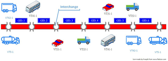
Figure 1.
Example: five vehicles (VT) travel on a road and pass gantries with identifiers (GID); “Reproduced with permission from 2017 International Conference on Applied System Innovation (ICASI); published by IEEE, 2017.”
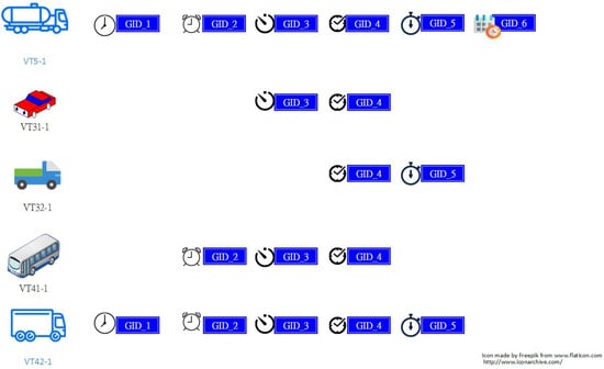
Figure 2.
Example: the gantry timestamp sequences of five vehicles according to the trips in Figure 1; “Reproduced with permission from 2017 International Conference on Applied System Innovation (ICASI); published by IEEE, 2017.”
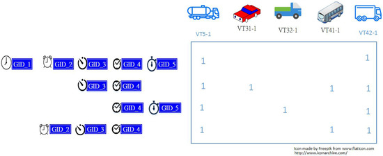
Figure 3.
Example: the significant travel time patterns extracted from the gentry timestamp sequences in Figure 2; “Reproduced with permission from 2017 International Conference on Applied System Innovation (ICASI); published by IEEE, 2017.”
To show the work of this study being practical, experimental resources are downloaded from the Traffic Data Collection System (TDCS),one of Taiwan government open data platforms. Experimental results contain the statistics of frequency distribution of vehicles passing through one selected gantry sequence according to 24 h per day; these statistics are expected to provide experts with hints to inspect traffic congestions and to help drivers how to avoid traffic jam. It is expected and attractive that this approach can provide the metadata of traffic patterns to enrich the effectiveness of dynamic traffic control strategies in the future.
2. Materials and Methods
2.1. Gantry Timestamp Sequences from Traffic Data Collection System (TDCS)
The timestamp gantry sequences in this study are extracted from the raw data “TDCS_M06A” of Traffic Data Collection System (TDCS) (http://tisvcloud.freeway.gov.tw/history/TDCS/), one of the Taiwan government open data platforms. Generally, each of the vehicles is usually attached with one electronic tag, as shown in Figure 4, on the front light of one car, as its identification for fee-charging; a timestamp associated with one gantry is recorded when that vehicle passes one gantry. Figure 5 shows one gantry “01F-196.0N”, for example, located at (N24.085622, E120.52785) in the northern direction of Freeway No. 1. Experimental resources, as shown in Table 1, that includes five months of gantry timestamp sequences collected from 2016/11 to 2017/3; the total size of 3624 files is about 103.0 GB. Table 2 shows some of records in the file “TDCS_M06A_20161101_000000.csv” collected at 2016/11/1, for example, and the field “TripInformation” is for storing the contents of timestamp gantry sequences of vehicles.

Figure 4.
Example: an electronic tag attached on the front light of one car.
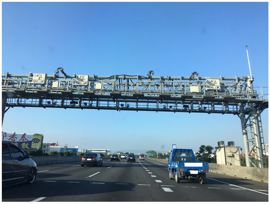
Figure 5.
Example: one gantry “01F-196.0N” in the northern direction of Freeway No. 1.

Table 1.
Experimental resources extracted from Traffic Data Collection System (TDCS).
Table 2.
Some records downloaded from Traffic Data Collection System (TDCS).
To make the contribution of this paper solidly, this study takes the longest trip, containing six gantries, from “05F-000.0S” to “05F-049.4S” (southern) or from “05F-052.8N” to “05F-000.1N” (northern) within the trips of Freeway No. 5 (Chiang Wei-shui Memorial Freeway), where that trip has been reported for a long time with serious traffic jam in the weekend or national holidays. Table 3 gives the details of these six gantries in both directions, the southern (S) from “05F-000.0S” to “05F-049.4S” and the northern (N) from “05F-052.8N” to “05F-000.1N”.
Table 3.
Six gantries in both of the southern and northern directions on Taiwan National Freeway No. 5.
2.2. Extracting Significant Travel Time Patterns and Computing the Statistics of These Patterns
The flowchart, as shown in Figure 6, includes two processes of extracting significant travel time patterns and computing the statistics of these patterns via Hadoop MapReduce programming. Section 2.2.1 and Section 2.2.2 give the details in the following.
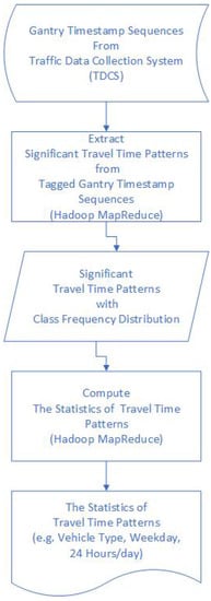
Figure 6.
The flowchart of extracting significant travel time patterns and computing the statistics of these patterns.
2.2.1. Extracting Significant Travel Time Patterns
The significant travel time patterns in this paper are defined as maximal repeats [8] that appear at least twice in gantry timestamp sequences and can not always be subsequence of the other patterns in these sequences. As shown in Figure 6, significant travel time patterns were extracted from gantry timestamp sequences downloaded from the “TDCS”; meanwhile, class frequency distribution of these patterns were computed. Note that the types of classes can be the combination of timestamp and vehicle types and are determined by observers or analyzers on purpose.
To have a significant travel time pattern extracted for illustration, Figure 7 (resp. Figure 8) gives one significant travel time pattern whose “Travel Time” is 34 min (resp. 39 min) extracted from the gantry timestamp sequences in the southern (resp. the northern) direction of Freeway No. 5. In Table 4, for example, some of the class frequency distributions of the significant travel time pattern in Figure 7 (resp. Figure 8) is in the 1st (resp. 4th) row. The format of class frequency distribution of one pattern in this study is defined as (“Date” “Weekday” “VehicleType”#“TF”), where the “Date” and “Weekday” present the date and the weekday that pattern happened, respectively, the “VehicleType” gives the type of vehicle, and the “TF” means the frequency of vehicles matching that case of class frequency distribution.
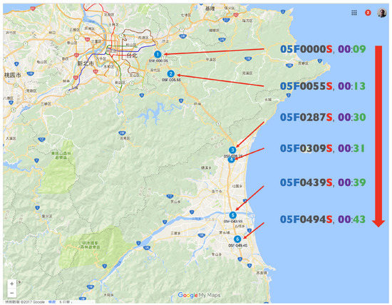
Figure 7.
Example: one travel time pattern in southern (S) direction from “05F0000S” to “05F0494S” (Travel Time = 34 min).
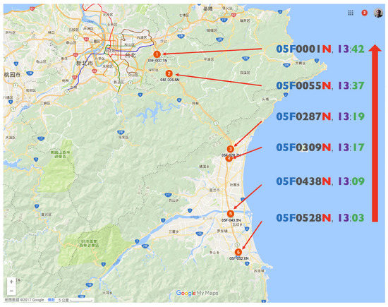
Figure 8.
Example: one travel time pattern in northern (N) direction from “05F0528N” to “05F0001N” (Travel Time = 39 min).
Table 4.
Examples of significant travel time patterns extracted from the Freeway No. 5 gantry timestamp sequences.
2.2.2. Computing the Statistics of Significant Travel Time Patterns
The class frequency distributions of significant travel time patterns, as shown in Figure 6, is the input of the process of computing the statistics of significant travel time patterns. The computation of these statistics via Hadoop MapReduce programming model is straightforward with the divide-and-conquer method [14] because this class frequency distribution of each pattern is independent from that of the others.
Table 4 gives four travel time patterns, for example, as the input for computing the statistics of significant travel time patterns extracted in Section 2.2.1. The travel time pattern, located in the 2nd row of Table 4, whose travel time interval was from 5:55 a.m. to 6:39 a.m. (travel time = 44 min) in the southern direction of Freeway No. 5. To take a closer view of class frequency distribution (“Date” “Weekday” “VehicleType”#”TF”) of that pattern, one can observe that there were seven (TF = 7) vehicles that consisted of four cars (VehicleType = 31) and three trucks (VehicleType = 32); moreover, it was interesting that these seven vehicles were almost in the same time period (minute) in the morning of the day “2017/01/28” (“Saturday”) when six gantries passed there. With this class frequency distribution of significant travel time patterns as described above, one can further obtain more specific observation from these metadata of traffic patterns according to what kind of frequency distribution he/she desires. Section 3 will give more experimental results in the following.
3. Results
To demonstrate the usages of the statistics of traffic patterns, this study chooses the longest trip in both the southern and northern directions of Taiwan freeway No. 5 and compares the frequency distributions of vehicles passing that trip according to 24 h per day. First of all, Section 3.1 gives a global view of class frequency distributions of vehicles according to two classes, the southern and the northern directions, respectively. To have more precise observation, Section 3.2 uses the combination of “24 h per day” and “seven days per week” as different classes. Similarly, Section 3.3 shows the class frequency distribution of vehicles according to different types of the combinations of “24 h per day” and “VehicleTypes”. Finally, Section 3.4 gives the average of travel time according to “24 h per day”. The details are described in the following.
3.1. The Frequency Distribution of Vehicles vs. “the Southern and Northern Directions”
Figure 9 gives the frequency distribution of vehicles according to “24 h per day” in both the southern and northern directions of Taiwan freeway No. 5. The rush hours in the southern and northern directions happened at 9:00 a.m. and 1:00 p.m., respectively. On the other hand, the summation of the frequency of vehicles in the southern direction was greater than that in the northern direction. That is, there might be many vehicles in the southern direction that didn’t start from the most southern gantry “05F–052.8N” when they came back in the northern direction.
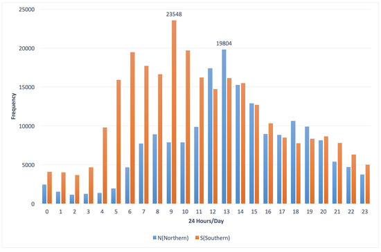
Figure 9.
The frequency distribution of vehicles in the S (southern) and N (northern) directions according to “24 h per day”.
3.2. The Frequency Distribution of Vehicles vs. “Seven Days per Week”
To observe the frequency distribution of vehicles in more detail, Figure 10 and Figure 11 take the seven days per week into consideration. Basically, the distribution in Figure 10 was similar to that in Figure 9, except that the frequency distribution of the “Sun” (Sunday) within the time period from 10:00 a.m. to 4:00 p.m. was much lower than that of the others. That is, one may have a smooth trip in the southern direction during that time period on Sunday. On the other hand, during the period from 8:00 a.m. to 4:00 p.m., as shown in Figure 11, the frequency distribution of the “Sat” (Saturday) was lower than that of the others. Most of all, there was a peak that happened at 5:00 p.m.; many people start their trips in the early morning of Saturday in the southern direction of Freeway No. 5. It is very interesting and attractive to have further investigation of social activities hidden in these events in the future.
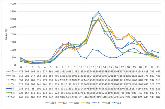
Figure 10.
The frequency distribution of vehicles in the southern (S) direction vs. “24 h per day” and “seven days per week”.
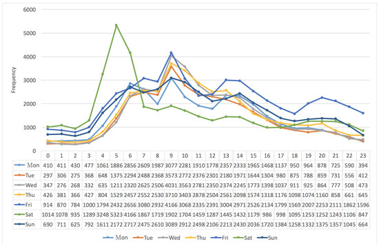
Figure 11.
The frequency distribution of vehicles in the northern (N) direction vs. “24 h per day” and “seven days per week”.
3.3. The Frequency Distribution of Vehicles vs. "VehicleTypes"
The “VehicleType” (VT), as shown in the first field of Table 2, includes five types as “5” (Trailer), “31” (Car/Sedan), “32” (Truck), “41” (Bus) and “42” (Big Truck). Figure 12 and Figure 13 present the frequency distribution of vehicles according to “24 h per day” and “VehicleType”; the first two popular types of vehicles are “31” (Car/Sedan) and “32” (Truck). The frequency distribution of the two types of vehicles, “5” (Trailer ) and “42” (Big Truck), are very low because they are strictly prohibited to enter some intervals containing tunnels without permission. By the way, as shown in Figure 13, most of the “41” (Bus) started their journey around 12:00 p.m. in the southern direction.
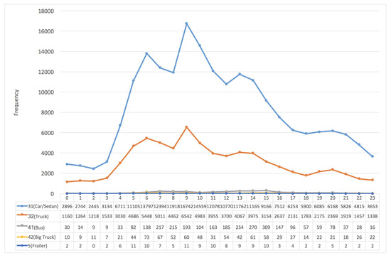
Figure 12.
The frequency distribution of vehicles in the southern (S) direction vs. “24 h per day” and “VehicleType”.
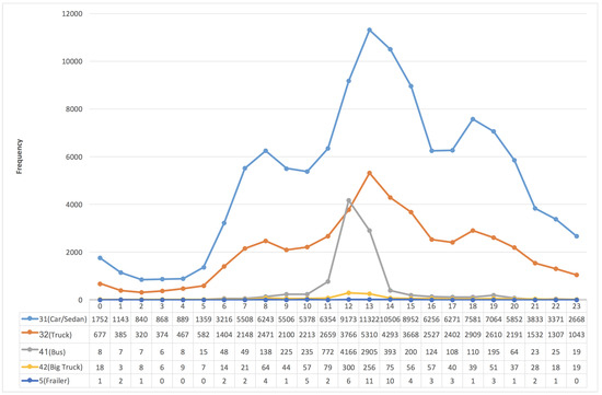
Figure 13.
The frequency distribution of vehicles in the northern (N) direction vs. “24 h per day” and “VehicleType”.
3.4. The Average of Travel Times vs. “Seven Days per Week”
It is expected to have the travel time distribution according to weekday or weekend. Figure 14 (resp. Figure 15) gives the average of travel times according to “seven days per week”. In the southern direction, Figure 14 shows that the average of travel time of the “Sat” (Saturday), ranging from 36 to 39 (min), during the time period from 6:00 a.m. to 4:00 p.m. On the other hand, Figure 15 shows that the “Sun” (Sunday) achieved the highest value (74 min) of average travel time during the time period from 2:00 p.m. to 3:00 p.m. Furthermore, it is interesting to know why the average travel time of the “Tue” and the “Wed” are higher than that of the others in the time period from 0:00 a.m. to 1:00 a.m.
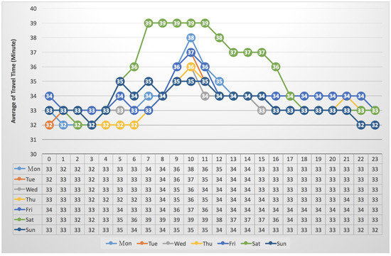
Figure 14.
The average of travel time of vehicles in the southern (S) direction vs. “24 h per day” and “seven days per week”.
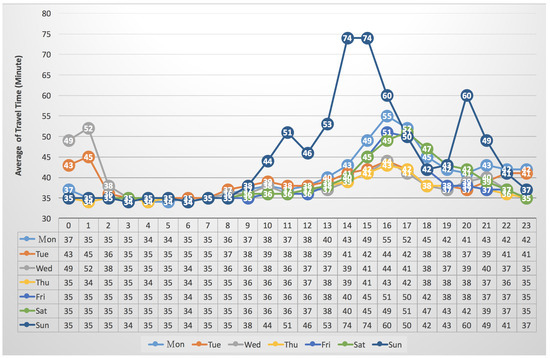
Figure 15.
The average of travel time of vehicles in the northern (N) direction vs. “24 h per day” and “seven days per week”.
3.5. Computational Time and Environment
Table 5 describes the hardware and software of a computing node; the environment for the Hadoop MapReduce computational platform contains eight nodes, two for the resource manager (name node) and six for worker nodes (data nodes). The total computational time of process “Extracting Significant Travel Time Patterns”, as shown in Table 6, is about “26h:36min:09s”; the process “Compute the statistics of Travel Time Patterns” is about “00h:3min:24s”.
Table 5.
Specifications of hardware and software within one computing node.
Table 6.
Computational time via a Hadoop cluster with two name nodes and six computing nodes.
4. Discussion
The analysis model of traffic flow theory [15,16,17,18,19,20] focused on describing the evolutionary behavior of traffic variables temporally and spatially. In historical studies [5,21], the statistics of traffic variables were collected and counted in aggregate based on a single detector observation. In modern traffic systems, or the so called intelligent transportation systems, vehicle detections are accomplished automatically via the transaction data of electronic devices of, which vehicle identification is widely available. With these records collected and the novel approach proposed in this paper, one can not only analyze the characteristics of traffic flow but also study the traffic congestion problem about the upstream propagation phenomenon such that he/she can have more precise observation about traffic flow from a microscopic point of view.
Due to the scalability of the previous work [7], it is believed that our approach can handle a larger amount of timestamp gantry sequences collected from a longer time period, e.g., several years. With these long-term and fine-grain statistics of travel time patterns of vehicles, the domain expects to have precise observation of vehicle behavior such that they can trace back to analyzing why these historical events resulted in traffic jam or congestion. Therefore, they can provide a new approach or police to avoid such a situation happening again in the future.
Indeed, there is still a lot of room for improving this study. First of all, an interactive data visualization interface, especially integrated with geographical map, is needed to promote the usage of these statistics as well as to stimulate users’ comprehension sensitively. Instead of “Hadoop” based on an external-memory method, on the other hand, “Spark”, an in-memory distributed computing, is expected to run 100× faster than Hadoop MapReduce.With the aid of cloud computing for sharing these statistics of travel time patterns in times, if possible, that are computed consistently via “Spark”, it may be attractive and expected to have this work as a software package, for providing current traffic information, integrated with IoT (Internet of Things) to make smart or driverless cars with more intelligence in the future.
5. Conclusions
This paper provides a novel approach, adopting a previous work based on the Hadoop MapReduce programming model, in order to extract significant travel time patterns from gantry timestamp sequences and, in the meantime, compute the class frequency distribution of these patterns, where the classes can be derived from the combination of timestamp and vehicle information according to what kind of distribution users desire to observe or analyze. Experimental resources include the timestamp gentry sequences of vehicles passed in five months from 2016/11 to 2017/3 that were downloaded from the Traffic Data Collection System (TDCS), one of the Taiwanese government’s open data platforms. The longest trip within Freeway No. 5, including six gantries in both the southern and northern directions, is selected for demonstration. Many kinds of class frequency distributions of significant travel time patterns are computed according to different combinations of time unit and vehicle information. The statistics, computed from the class frequency distribution, did reveal some interesting and valuable information about traffic and transportation issues for further research or analysis.
Acknowledgments
This study is partially supported by the Ministry of Science and Technology, Taiwan under project MOST 105-2632-E-468-002.
Author Contributions
Jing-Doo Wang conceived and designed the experiments, and wrote the paper; Ming-Chorng Hwang provided the background of traffic and transportation research, and suggested how to use the records in the Traffic Data Collection System (TDCS); both Jing-Doo Wang and Ming-Chorng Hwang analyzed and discussed experimental results.
Conflicts of Interest
The authors declare no conflict of interest.
References
- Braess, D. Über ein Paradoxon aus der Verkehrsplanung. Unternehmensforschung 1968, 12, 258–268. [Google Scholar] [CrossRef]
- Braess, D.; Nagurney, A.; Wakolbinger, T. On a Paradox of Traffic Planning. Transp. Sci. 2005, 39, 446–450. [Google Scholar] [CrossRef]
- Dafermos, S.; Nagurney, A. On some traffic equilibrium theory paradoxes. Transp. Res. Part B 1984, 18, 101–110. [Google Scholar] [CrossRef]
- Hwang, M.C.; Cho, H.J. The Classical Braess Paradox Problem Revisited: A Generalized Inverse Method on Non-Unique Path Flow Cases. Netw. Spat. Econ. 2016, 16, 605–622. [Google Scholar] [CrossRef]
- Vlahogianni, E.I.; Karlaftis, M.G.; Golias, J.C. Short-term traffic forecasting: Where we are and where we’re going. Transp. Res. Part C 2014, 43 Pt 1, 3–19. [Google Scholar] [CrossRef]
- Wang, J.D.; Hwang, M.C. A Novel Approach to Extract Significant Time Intervals of Vehicles from Superhighway Gantry Timestamp Sequences. In Proceedings of the 2017 IEEE International Conference on Applied System Innovation, Sapporo, Japan, 13–17 May 2017; pp. 1679–1682. [Google Scholar]
- Wang, J.D. Extracting significant pattern histories from timestamped texts using MapReduce. J. Supercomput. 2016, 72, 3236–3260. [Google Scholar] [CrossRef]
- Gusfield, D. Algorithms on Strings, Trees, and Sequences : Computer Science and Computational Biology; Cambridge University Press: Cambridge, UK, 1997. [Google Scholar]
- Gunarathne, T. Hadoop MapReduce v2 Cookbook, 2nd ed.; Packt Publishing: Birmingham, UK, 2015. [Google Scholar]
- Wang, J.D. External memory approach to compute the maximal repeats across classes from DNA sequences. Asian J. Health Inf. Sci. 2006, 1, 276–295. [Google Scholar]
- Li, F.; Ooi, B.C.; Özsu, M.T.; Wu, S. Distributed Data Management Using MapReduce. ACM Comput. Surv. 2014, 46, 31:1–31:42. [Google Scholar] [CrossRef]
- Qin, L.; Yu, J.X.; Chang, L.; Cheng, H.; Zhang, C.; Lin, X. Scalable Big Graph Processing in MapReduce. In Proceedings of the 2014 ACM SIGMOD International Conference on Management of Data, Snowbird, UT, USA, 22–27 June 2014; pp. 827–838. [Google Scholar]
- Tan, Y.S.; Tan, J.; Chng, E.S.; Lee, B.S.; Li, J.; Date, S.; Chak, H.P.; Xiao, X.; Narishige, A. Hadoop framework: Impact of data organization on performance. Software 2013, 43, 1241–1260. [Google Scholar] [CrossRef]
- Cormen, T.H.; Leiserson, C.E.; Rivest, R.L.; Stein, C. Introduction to Algorithms, 3rd ed.; MIT Press: Cambridge, MA, USA, 2009. [Google Scholar]
- Gerlough, D.; Huber, M. Traffic Flow Theory: A Monograph; Number 165 in Special Report; No. 165; Transportation Research Board, National Research Council: Washington, DC, USA, 1975.
- Ferrari, P. The reliability of the motorway transport system. Transp. Res. Part B 1988, 22, 291–310. [Google Scholar] [CrossRef]
- Elefteriadou, L. An Introduction to Traffic Flow Theory; Springer: Berlin, Germany, 2014. [Google Scholar]
- Kerner, B. Introduction to Modern Traffic Flow Theory and Control: The Long Road to Three-Phase Traffic Theory; Springer: Berlin/Heidelberg, Germany, 2014. [Google Scholar]
- Mauro, R.; Cattani, M.; Guerrieri, M. Evaluation of the safety performance of turbo roundabouts by means of a potential accident rate model. Baltic J. Road Bridge Eng. 2015, 10, 28–38. [Google Scholar] [CrossRef]
- Guerrieri, M.; Mauro, R. Capacity and safety analysis of hard-shoulder running (HSR). A motorway case study. Transp. Res. Part A 2016, 92, 162–183. [Google Scholar] [CrossRef]
- Zhang, Y. Special issue on short-term traffic flow forecasting. Transp. Res. Part C 2014, 43 Pt 1, 1–2. [Google Scholar] [CrossRef]
© 2017 by the authors. Licensee MDPI, Basel, Switzerland. This article is an open access article distributed under the terms and conditions of the Creative Commons Attribution (CC BY) license (http://creativecommons.org/licenses/by/4.0/).