Tuning Guidelines for an Adaptive-Gain Parabolic Sliding Mode Filter

Abstract

This paper quantitatively evaluates the performance of an adaptive-gain parabolic sliding mode filter (AG-PSMF), which is for removing noise in feedback control of mechatronic systems under different parameter values and noise intensities. The evaluation results show that, due to the nonlinearity of AG-PSMF, four performance measurements, i.e., transient time, overshoot magnitude, tracking error and computational time, vary widely under different conditions. Based on the evaluation results, the paper provides practical tuning guidelines for AG-PSMF to balance the tradeoff among the four measurements. The effectiveness of the guidelines is validated through numerical examples.

1. Introduction

The sliding mode filter [1,2] employing a certain kind of parabolic-shaped sliding surface has been studied for effectively removing noise in feedback control of mechatronic systems. One of major advantages of the filter is that its output converges to the input when a constant input is provided. In addition, the filter does not require a dynamic model. The sliding mode filter has been recognized one of the most effective and robust filters, and its evaluation results [3,4,5] and applications [6,7,8,9,10,11,12,13,14] have been reported in the literature. However, the filter is prone to overshooting.

In response to the drawbacks of the sliding mode filter [1,2], Jin et al. [15] presented a new parabolic sliding mode filter, which is referred to as PSMF. It is reported [16,17] that PSMF is advantageous over the filter referred to in [1,2] and linear filters because it is less prone to overshooting and produces smaller phase lag. After that, Jin et al. [18] presented an adaptive-gain parabolic sliding mode filter, referred to as AG-PSMF, by extending PMSF. In that work, Jin et al. stated that AG-PSMF effectively removes noise by balancing the tradeoff between the filtering smoothness and the suppression of delay [18]. However, due to the strong nonlinearity, theoretical evaluation and corresponding result-based parameter tuning guidelines remained as open problems for future study.

To respond to these problems, in an alternative manner this paper provides insight into the issues of quantitative performance evaluation and parameter tuning of AG-PSMF through numerical analysis. Specifically, the contribution of the paper is two-fold. It (1) quantitatively evaluates the performance of AG-PSMF under different parameter values and input signals; and (2) based on the results of the quantitative evaluation, the paper presents practical tuning guidelines for AG-PSMF.

The rest of this paper is organized as follows: Section 2 provides an overview of parabolic sliding mode filters; Section 3 quantitatively evaluates the performance of AG-PSMF; Section 4 presents tuning guidelines of AG-PSMF based on the evaluation results; Section 5 validates the effectiveness of the presented guidelines through numerical examples; and Section 6 covers concluding remarks.

2. Parabolic Sliding Mode Filters

This section provides an overview of parabolic sliding mode filters for understanding of the presented analysis in the following sections.

In Reference [15], Jin et al. presented a sliding mode filter that employs a parabolic-shaped sliding surface (PSMF), of which continuous-time representation is given as follows:

$$\begin{array}{}(1\mathrm{a})& \hfill {\dot{x}}_1& =& x_2\hfill (1\mathrm{b})& \hfill {\dot{x}}_2& \in & -\frac{F(H+1)}{2}\mathrm{sgn}(\sigma (F,u,x_1,x_2))-\frac{F(H-1)}{2}\mathrm{sgn}(x_2),\hfill \end{array}$$

where

$$\begin{array}{c}\hfill \sigma (F,u,x_1,x_2)\triangleq 2F(x_1-u)+|x_2|x_2,\end{array}$$

(2)

$u\in \mathbb{R}$ is the input, $x_1\in \mathbb{R}$ is the output, $x_2\in \mathbb{R}$ is the derivative of $x_1$, and $F>0$ and $H>1$ are constants. In addition, $\mathrm{sgn}()$ is the following set-valued signum function:

$$\begin{array}{c}\hfill \mathrm{sgn}(z)\triangleq \left\{\begin{array}{cc}1\hfill & \mathrm{if}z>0\hfill \\ [-1,1]\hfill & \mathrm{if}z=0\hfill \\ -1\hfill & \mathrm{if}z<0,\hfill \end{array}\right.\end{array}$$

(3)

where $z\in \mathbb{R}$ is a scalar. Figure 1 shows the sliding surface and state trajectories of PSMF in $x_1$–$x_2$ space. In PSMF, ${\dot{x}}_2$ can be seen as the acceleration of the output $x_1$, and F can be considered as the gain of the acceleration.

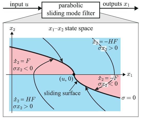
Figure 1. The parabolic-shaped sliding surface (thick curve) and trajectories of the state of the parabolic sliding mode filter (PMSF) (thin curve).

The paper [15] also presented the following discrete-time algorithm of PSMF, which is derived by using the backward Euler discretization (i.e., by replacing $x_2$ by $(x_1(k)-x_1(k-1))/T$):

Algorithm 1 PSMF

1: ${\displaystyle x_2^{*}:=FT\Phi \left(\frac{u(k)-x_1(k-1)}{F{T}^2}\right)}$ 2: $x_2(k):=\mathrm{clip}(\mathrm{clip}(x_2(k-1)-HFT,x_2(k-1)-FT,0),\mathrm{clip}(x_2(k-1)+FT,x_2(k-1)+FTH,0),x_2^{*})$ 3: $x_1(k):=x_1(k-1)+T{x}_2(k)$ 4: $\mathbf{RETURN}{x}_1(k)$.

Here, T is the sampling interval, k is the discrete-time index, and $\Phi ()$ and $\mathrm{clip}()$ are functions defined as follows:

$$\begin{array}{c}\hfill \Phi (z)\triangleq \mathrm{sgn}(z)\left(\sqrt{1+2|z|}-1\right),\end{array}$$

(4)

$$\begin{array}{c}\hfill \mathrm{clip}(a,b,z)\triangleq \left\{\begin{array}{cc}b\hfill & \mathrm{if}z>b\hfill \\ z\hfill & \mathrm{if}z\in [a,b]\hfill \\ a\hfill & \mathrm{if}z<a,\hfill \end{array}\right.\end{array}$$

(5)

where $a\in \mathbb{R}$ and $b\in \mathbb{R}$ satisfy $a\le b$. In Algorithm 1, $x_2^{*}(k)$ is the value of $x_2(k)$ that satisfies $\sigma (k)=0$, and $x_2(k)$ is determined in order to follow $x_2^{*}(k)$ under the constraint of acceleration. It should be mentioned that, owing to the use of backward Euler discretization, the discrete-time implementation of PSMF does not produce chattering, which has been considered as a common problem of sliding mode techniques.

It is reported [16,17] that the noise removing capability of PSMF is almost the same as that of second-order Butterworth low-pass filter (2-LPF), but PSMF produces smaller phase lag than 2-LPF does. In addition, compared with the filter in [1,2], PSMF produces smaller phase lag , and it is less prone to overshooting. The effectiveness of PSMF has been experimentally validated [16,17]. However, due to the fixed acceleration gain F, the output of PSMF cannot follow an input in which the acceleration exceeds that of PSMF, whereas the output becomes sensitive to the noise contained in the input of which acceleration is far below that of PSMF.

With respect to the above-mentioned limitation of PSMF, Jin et al. presented an adaptive-gain parabolic sliding mode filter (AG-PSMF), which is an extension of PSMF. Specifically, the complete algorithm of AG-PSMF is given as follows:

Algorithm 2 Adaptive gain parabolic sliding mode filter (AG-PMSF)

1: $\mathrm{FOR}n\in \{1,\cdots ,\min (k+1,N_{\max })\}$   2: $v:=(x_1(k-1)-x_1(k-n-1))/(nT)$   3: $\mathrm{FOR}i\in \{1,\cdots ,n\}$   4: $e:=x_1(k-i-1)-x_1(k-1)+iTv$   5: $\mathrm{IF}|e|>R;\text{EXIT LOOP}$   6: $\text{END FOR}$   7: $\mathrm{IF}i<n;\text{EXIT LOOP}$   8: $\text{END FOR}$   9: ${\displaystyle F^{*}=\frac{N_{\max }}{2n}F}$ 10: ${\displaystyle x_2^{*}:=F^{*}T\Phi \left(\frac{u(k)-x_1(k-1)}{F^{*}{T}^2}\right)}$ 11: $x_2(k):=\mathrm{clip}(\mathrm{clip}(x_2(k-1)-H{F}^{*}T,x_2(k-1)-F^{*}T,0),\mathrm{clip}(x_2(k-1)+F^{*}T,x_2(k-1)+F^{*}TH,0),x_2^{*})$ 12: $x_1(k):=x_1(k-1)+T{x}_2(k)$ 13: $\mathbf{RETURN}{x}_1(k)$.

In AG-PSMF, i.e., Algorithm 2, steps 1–8 check whether all previous outputs are inside the area determined by the two end-outputs $x_1(k-1)$ and $x_1(k-n-1)$ and the constant R, as shown in Figure 2. If it is the case, the window size n is further increased. The increase of n is continued until at least one previous output lies outside the area or n reaches its maximum value $N_{\max }$. Then, in step 9, gain $F^{*}(k)$ is obtained by applying the adaptively determined window size for balancing the tradeoff the output smoothness and the suppression of delay.

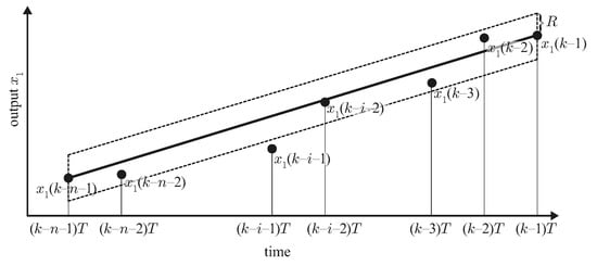
Figure 2. Windowing in adaptive-gain (AG)-PSMF.

3. Performance Evaluation of AG-PSMF

This section numerically evaluates the performance of AG-PSMF under different values of parameters and noise intensities. It should mentioned here that, in the upcoming analysis, parameter values are changed in ranges that capture the response tendencies of AG-PSMF, without loss of generality. In addition, $F=1000$ and $T=0.0001$ s are used for the discrete-time implementation of AG-PSMF.

3.1. Transient Time and Overshoot Magnitude for Different Values of H

This part investigates the transient time and the overshoot magnitude produced by AG-PSMF with the following input:

$$\begin{array}{c}\hfill u=1+\alpha \epsilon (t),\end{array}$$

(6)

where $\epsilon \sim \mathcal{N}(0,1)$ is the unit white Gaussian noise with zero mean, and α is a normalized noise-scaling constant. Here, as shown in Figure 3, the transient time is defined as the time required for the output to reach 90 % of the signal component of the input, i.e., the input amplitude with $\alpha =0$. In addition, the overshoot magnitude is defined as the maximum amount of the output that measured upward from the signal component of the input.

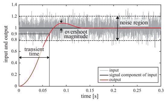
Figure 3. Response of AG-PSMF with input $u=1+0.1\epsilon (t)$ under $H=1.5$, $N_{\max }=25$ and $R=0.001$.

Figure 4 and Figure 5 show the transient time and the overshoot magnitude , respectively, under different values of H and α. In addition, Figure 6 provides cross-section view of Figure 4 and Figure 5 under $\alpha =0.1$. It is shown that the overshoot magnitude decreases as H increases, and it converges to a certain value in the range of $H\ge 5$. On the other hand, the increase of H results in longer transient time, which dramatically increases within the range of $H>10$. Such tendencies become stronger as the value of α increases.

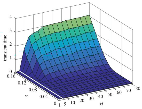
Figure 4. Transient time with input $u=1+\alpha \epsilon (t)$ under different values of H and α.

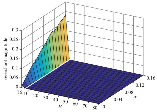
Figure 5. Overshoot magnitude with input $u=1+\alpha \epsilon (t)$ under different values of H and α.

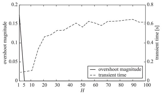
Figure 6. Cross-section view of overshoot magnitude and transient time with input $u=1+0.1\epsilon (t)$ under different values of H.

3.2. Tracking Accuracy for Different Values of $N_{\max }$ and R

This part evaluates the tracking performance of AG-PSMF under the following input:

$$\begin{array}{c}\hfill u=\sin (10t)+\alpha \epsilon (t),0\mathrm{s}\le t\le 4.2\mathrm{s}.\end{array}$$

(7)

The performance is analyzed through the average magnitude of $|\widehat{u}-x_1|$ (AME), which is defined as follows:

$$\begin{array}{c}\hfill \mathrm{AME}\triangleq \frac{1}{42000}{\displaystyle \sum _{k=0}^{42000}}|\widehat{u}-x_1|,\end{array}$$

(8)

where $\widehat{u}$ is the signal component of the input, i.e., $\widehat{u}=\sin (10t)$.

Figure 7 shows AME under different values of $N_{\max }$ and α, and Figure 8 provides AME of Figure 7 under $\alpha =0.1$. One can observe that AME converges to its minimum value as $N_{\max }$ reaches around $N_{\max }=50$ under a certain value of α.

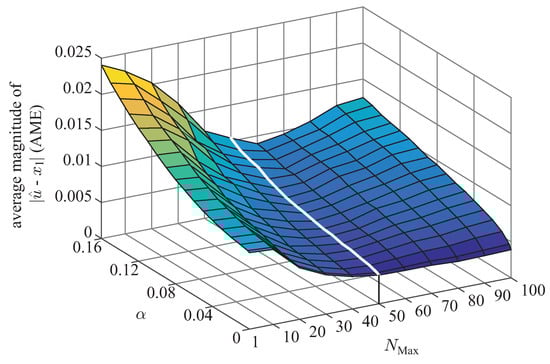
Figure 7. Average magnitude of $|\widehat{u}-x_1|$ (AME) with input $u=\sin (10t)+\alpha \epsilon (t)$ under different values of $N_{\max }$ and α.

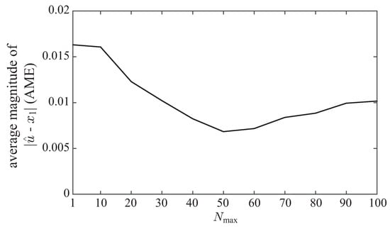
Figure 8. Average magnitude of $|\widehat{u}-x_1|$ (AME) with input $u=\sin (10t)+0.1\epsilon (t)$ under different value of $N_{\max }$.

The influence of R is shown in Figure 9, which gives AME for different values of R and α. In addition, Figure 10 provides AME of Figure 9 under $\alpha =0.1$. It is shown that, under a certain value of α, AME dramatically increases and converges to a certain value as R increases in the range $R>0.0001$. On the other hand, in the case of $R<0.0001$, AG-PSMF produces smaller AME than that of the case $R>0.0001$, but the value is slightly larger compared with the case of $R=0.0001$.

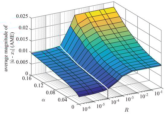
Figure 9. Average magnitude of $|\widehat{u}-x_1|$ (AME) with input $u=\sin (10t)+\alpha \epsilon (t)$ under different values of R and α.

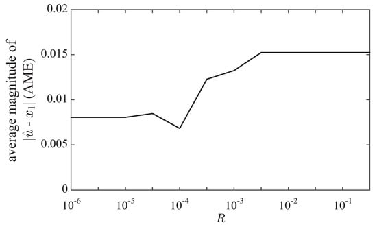
Figure 10. Average magnitude of $|\widehat{u}-x_1|$ (AME) with input $u=\sin (10t)+0.1\epsilon (t)$ under different values of R.

The figures also show that stronger noise intensity results in larger AME for a certain value of $N_{\max }$ and R.

3.3. Computational Time for Different Values of $N_{max}$ and R

Figure 11 shows the computational time spent by AG-PSMF with the input (7) under different values of $N_{\max }$ and R. It is shown that the influence R on the computational time is insignificant in the range $R\le 0.0001$. In this range, the computational time under $10\le N_{\max }\le 40$ is slightly less than that under $N_{\max }>40$, as shown in Figure 12. However, in the range $R>0.0001$, the computational time increases with either increase in $N_{\max }$ or R.

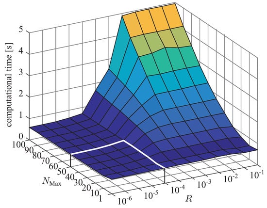
Figure 11. Computational time with input $u=\sin (10t)+0.1\epsilon (t)$ under different values of $N_{\max }$ and R.

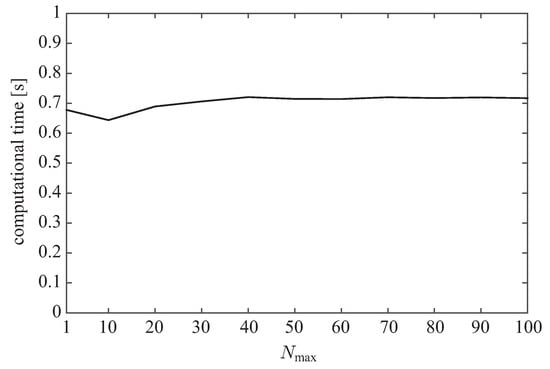
Figure 12. Computational time with input $u=\sin (10t)+0.1\epsilon (t)$ under different values of $N_{\max }$ and $R=0.0001$.

4. Tuning Guidelines of AG-PSMF

In practice, parameter values greatly influence system performances, and thus parameter tuning guidelines are important for systems to perform properly. However, in the case of AG-PSMF, the tuning of algorithm parameters remains empirical due to the difficulty of theoretical evaluation caused by strong nonlinearity.

In response to this problem, as an alternative solution this section provides parameter tuning guidelines for AG-PSMF based on the results of numerical evaluation given in Section 3. Specifically, the guidelines focus on the influence of different values of AG-PSMF’s three parameters H, $N_{\max }$ and R on the four measurements transient time, overshoot magnitude, tracking error (i.e., AME) and computational time. It should be said that, for a better filtering performance, the values of all four measurements should be kept small. Given this requirement, tuning guidelines for AG-PSMF’s parameters are derived as follows.

4.1. Tuning Guideline for H

In Section 3.1, it has been discussed that the increase of H contributes to the suppression of overshoot but results in longer transient time. By carefully observing the response of AG-PSMF under different values of H, as shown in Figure 4, Figure 5 and Figure 6, one can notice that the optimum range of H is around $5\le H\le 10$. Under such a value of H, AG-PSMF provides short transient time by producing a low level of overshoot.

4.2. Tuning Guideline for $N_{\max }$

In Section 3.2, it has been shown that the minimum AME appears around $N_{\max }=50$. Thus, it is suggested that $N_{\max }$ should be set as around $N_{\max }=50$. However, in the applications where the computational time is a major concern, it is advisable to set around $20\le N_{\max }\le 30$ by considering the results of Section 3.3. This is because under such values of $N_{\max }$, AG-PSMF consumes slightly less computational cost while maintaining relatively low level of AME.

4.3. Tuning Guideline for R

In Section 3.2, it has been observed that AME converges to the minimum value as R approaches $R=0.0001$. On the other hand, in Section 3.3, it has been illustrated the the computational time is insignificant in the range of $R\le 0.0001$, while it increases with the increase of R in the range $R>0.0001$. Thus, it is clear that the value of R around $R=0.0001$ should be appropriate by considering both AME and computational time.

5. Numerical Examples

The effectiveness of the presented guidelines are now validated through numerical examples, the following sinusoidal signal is provided as the input of AG-PSMF:

$$\begin{array}{c}\hfill u=\left\{\begin{array}{cc}\sin (20)+0.1\epsilon (t)\hfill & \mathrm{if}t\le 1.5\mathrm{s},\hfill \\ 2\sin (20t)+0.1\epsilon (t)\hfill & \mathrm{if}1.5\mathrm{s}<t\le 3\mathrm{s},\hfill \\ \sin (40t)+0.1\epsilon (t)\hfill & \mathrm{otherwise}.\hfill \end{array}\right.\end{array}$$

(9)

According to the guidelines, the values of parameters are set as $H=5$, $N_{\max }=50$, and $R=0.0001$. Besides that, $F=1000$ and $T=0.0001$ s are applied.

Figure 13 shows the output of AG-PSMF under the parameter values recommended by the guidelines (hereafter denoted as the AG-PSMF Guideline). For comparison, the results of AG-PSMF with four different sets of parameter values are also included. The initial states of all conditions are set zeros at $t=0$ s. The results clearly show the advantage of using $H>1$. That is, the AG-PSMF Guideline is less prone to overshooting than in the case of $H=1$. In addition, compared with the cases of $N_{\max }=25$ and $R=0.001$, the output amplitude of the AG-PSMF Guideline is closer to that of signal component of the input. Furthermore, the phase lag of the AG-PSMF-Guideline is the smallest among the four cases. As a whole, one can conclude that AG-PSMF performs the best under the recommended parameter values.

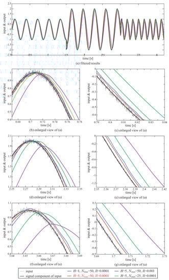
Figure 13. Outputs of AG-PSMF under different values of parameters for a sinusoidal input that is corrupted by white Gaussian noise.

6. Conclusions

This paper has quantitatively evaluated the performance of an adaptive-gain parabolic sliding mode filter (AG-PSMF) for removing noise in feedback control of mechatronic systems, under different parameter values and noise intensities. The evaluation results show that, due to the nonlinearity, the performance of AG-PSMF varies widely under different conditions. Based on the evaluation results, the paper has provided practical tuning guidelines for AG-PSMF to optimize performance. The effectiveness of the guidelines is validated through numerical examples.

One issue that remains for future study is theoretical validation of AG-PSMF.

References

- Han, J.; Wang, W. Nonlinear tracking-differentiator. J. Syst. Sci. Math. Sci. 1994, 14, 177–183. (In Chinese) [Google Scholar]
- Emaru, T.; Tsuchiya, T. Research on estimating smoothed value and differential value by using sliding mode system. IEEE Trans. Robot. Autom. 2003, 19, 391–402. [Google Scholar] [CrossRef]
- Han, J.; Huang, Y. Frequency characteristic of second-order tracking-differentiator. Math. Pract. Theory 2003, 33, 71–74. (In Chinese) [Google Scholar]
- Emaru, T.; Tsuchiya, T. Research on signal tracking performance of nonlinear digital filter ESDS. Trans. Jpn. Soc. Mech. Eng. Ser. C 2004, 70, 2352–2359. (In Japanese) [Google Scholar] [CrossRef]
- Guo, B.; Zhao, Z. On convergence of tracking differentiator. Int. J. Control 2011, 84, 693–701. [Google Scholar] [CrossRef]
- Su, Y.; Duan, B.; Zheng, C. Nonlinear PID control of a six-DOF parallel manipulator. IEEE Proc. Control Theory Appl. 2004, 151, 95–102. [Google Scholar] [CrossRef]
- Su, Y.; Sun, D.; Duan, B. Design of an enhanced nonlinear PID controller. Mechatronics 2005, 15, 1005–1024. [Google Scholar] [CrossRef]
- Peng, X.; Cheng, S.; Wen, J. Application of nonlinear PID controller in superconducting magnetic energy storage. Int. J. Control Autom. Syst. 2005, 3, 296–301. [Google Scholar]
- Han, J. From PID to active disturbance rejection control. IEEE Trans. Ind. Electron. 2009, 56, 900–906. [Google Scholar] [CrossRef]
- Xia, Y.; Fu, M. Overview of ADRC. Compd. Control Methodol. Flight Veh. 2013, 438, 21–48. [Google Scholar]
- Duan, X.; Qiu, Y.; Mi, J.; Zhao, Z. Motion prediction and supervisory control of the macro-micro parallel manipulator system. Robotica 2011, 29, 1005–1015. [Google Scholar] [CrossRef]
- Su, Y.; Duan, B.; Zheng, C.; Chen, G.; Mi, J. Disturbance-rejection high-precision motion control of a Stewart platform. IEEE Trans. Control Syst. Technol. 2004, 12, 364–374. [Google Scholar] [CrossRef]
- Sun, D. Comments on active disturbance rejection control. IEEE Trans. Ind. Electron. 2007, 6, 3428–3429. [Google Scholar]
- Xia, Y.; Shi, P.; Rees, D.; Han, J. Active disturbance rejection control for uncertain multivariable systems with time-delay. IET Control Theory Appl. 2007, 1, 75–81. [Google Scholar] [CrossRef]
- Jin, S.; Kikuuwe, R.; Yamamoto, M. Real-time quadratic sliding mode filter for removing noise. Adv. Robot. 2012, 26, 877–896. [Google Scholar]
- Jin, S.; Kikuuwe, R.; Yamamoto, M. Parameter selection guidelines for a parabolic sliding mode filter based on frequency and time domain characteristics. J. Control Sci. Eng. 2012, 2012, 923679. [Google Scholar] [CrossRef]
- Jin, S.; Kikuuwe, R.; Yamamoto, M. Improved velocity feedback for position control by using a quadratic sliding mode filter. In Proceedings of the 11th International Conference on Control, Automation and Systems, Gyeonggi-do, Korea, 26–29 October 2011; pp. 1207–1212.
- Jin, S.; Jin, Y.; Wang, X.; Xiong, X. Discrete-Time Sliding Mode Filter with Adaptive Gain. Appl. Sci. 2016, 6, 400. [Google Scholar] [CrossRef]
© 2017 by the authors. Licensee MDPI, Basel, Switzerland. This article is an open access article distributed under the terms and conditions of the Creative Commons Attribution (CC BY) license ( http://creativecommons.org/licenses/by/4.0/).