Abstract
This paper proposes proportional-integral/proportional gain controller parameter tuning in a two-degrees-of-freedom (2DOF) control system using the fictitious reference iterative tuning (FRIT) method for permanent magnet synchronous motor (PMSM) speed control using a field-programmable gate array (FPGA) for a high-frequency SiC MOSFET (metal oxide semiconductor field-effect transistor) inverter. The PI-P (proportional-integral/proportional) controller parameters can be tuned using the FRIT method from one-shot experimental data without using a mathematical model of the plant. Particle swarm optimization is used for FRIT optimization. An inverter that uses a SiC MOSFET is presented to achieve high-frequency operation at up to100 kHz using a switching pulse-width modulation (PWM) technique. As a result, a high-responsivity and high-stability PMSM (permanent magnet synchronous motor) control system is achieved, where the speed response follows the ideal response characteristic for both the step response and the disturbance response. High-responsivity and optimal disturbance rejection can be achieved using the 2DOF control system. FPGA-based digital hardware control is used to maximize the switching frequency of the SiC MOSFET inverter. Finally, an experimental system is set up, and experimental results are presented to prove the viability of the proposed method.
1. Introduction
This paper presents the use of the fictitious reference iterative tuning (FRIT) method for tuning of a two-degree-of-freedom (2DOF) proportional-integral/proportional (PI-P) controller in a new speed control system for a permanent magnet synchronous motor (PMSM) using a field-programmable gate array (FPGA) for a high-frequency SiC MOSFET (metal oxide semiconductor field-effect transistor) inverter. High-switching frequency operation can be achieved using the SiC MOSFET because of its superior material characteristics [1,2,3,4]. Variable-frequency drives (VFDs) can be operated efficiently at carrier frequencies in the 50 to 200 kHz range when using this device [5]. PI-P controller is feedback-type (FB-type) 2DOF control system. The 2DOF PI-P controller offers a powerful way to make both the set-point response and the disturbance response practically optimal [6].
FPGA-based digital hardware control is used to ensure fast processing operation for the high-frequency switching of the SiC MOSFET inverter. FPGA has advantages, such as high-speed processing and rewritablility. High-speed calculation is obtained using the ability of hardware processing. The synthesis process, the generate programming file process and the configure target device process must be performed before downloading the programming file to an FPGA, so that it is not effective nor efficient to tune PI-P controller parameters only to determine the value of controller parameters by trial and error. It takes several times of tuning the PI-P controller parameters. To overcome this problem, the FRIT method is used to tune PI-P controller parameters, which require one-shot experimental data, so tuning PI-P controller parameters is effective and efficient.
A high-performance motor control system requires a high-responsivity system and immediate recovery to the steady-state condition when a motor under load is affected by any disturbance [7]. To achieve this aim, a high-frequency pulse-width modulation (PWM) method is needed when using the SiC MOSFET inverter. High-responsivity and optimal disturbance rejection can be achieved using the 2DOF control system with high-frequency PWM. There are many advantages to using high- frequency PWM (in the 50 to 100 kHz range) in motor drive applications, including high motor efficiency, fast control response, reduced motor torque ripple, near-ideal sinusoidal motor current waveforms, reduced filter sizes and lower filter costs [5].
Recently, FRIT, which can be used to obtain optimal controller parameters using the input and output data from one-shot experimental data, has been studied by several researchers [8,9,10,11,12,13,14,15,16,17]. The data are used to determine the plant dynamics without knowing the mathematical model of the plant [13]. FRIT is used to obtain optimal controller parameters by optimizing a performance index that consists of the squared error between reference and experimental outputs.
Many published studies that have considered direct control parameter tuning methods, such as iterative feedback tuning (IFT), virtual reference iterative tuning (VRFT) and fictitious reference iterative tuning (FRIT). Hjalmarson [18] developed iterative feedback tuning. This requires signal and gradient quantities to achieve optimal performance. It also performs many experiments to update the controller parameters to minimize the performance index, so that it is not effective nor efficient to tune controller parameters, because it takes several times and costs. Campi et al. [19] proposed virtual reference feedback tuning (VRFT); Lecchini et al. [20] proposed 2DOF VRFT; Rojas et al. [21] proposed a feedforward formulation of the VRFT method based on a 2DOF control configuration; and Gazdos et al. [22] proposed a VRFT method for iterative controller design and fine tuning. VRFT uses a set of measured input/output data for the design of a controller with the desired structure, but without restrictions on data generation. It is based on the idea of constructing a virtual reference signal and on model reference control. The performance index is minimized using input data, and pre-filtering in VRFT requires the desired closed loop response and its sensitivity function. Both FRIT and VRFT have similar ideas and reference signals, where the fictitious reference signal is for FRIT and the virtual reference signal is for VRFT. Both FRIT and VRFT have similar performance index formulas and purposes to obtain the optimal controller parameter by minimizing the performance index using input and output data taken from a one-shot experiment. The performance index of VRFT focuses on the input, while the performance index of FRIT focuses on the output, so that FRIT is more understandable than VRFT [13]. The FRIT method is easier to use in this research than the VRFT method because the performance index used focuses on the output, and researchers give more attention to the FRIT method than the VRFT method to design the controller parameters. VRFT and FRIT only need one-shot experimental data to obtain the optimal controller parameters, so VRFT and FRIT are more effective or efficient than IFT. The FRIT method is easier to implement than the VRFT method to obtain the controller parameter of PMSM speed control. The step reference model and disturbance reference model can be formed following the output data in the FRIT method, but these reference model cannot be formed following the input data in the VRFT method like the input data of the PMSM speed control. The FRIT method is very useful to implement to obtain the optimal controller parameter of PMSM speed control. Soma et al. [8,9] proposed FRIT; Wakasa et al. [10] proposed an online-type controller parameter tuning method based on modification of the standard FRIT; and Azuma et al. [11] proposed the FRIT-particle swarm optimization (FRIT-PSO) method to design proportional-integral-derivative (PID) controllers for control systems. These researchers studied tuning methods using FRIT in a one-degree-of-freedom control system. Kaneko et al. [12,13,14,15] proposed the use of the FRIT method for tuning of the feedforward controller in a 2DOF control system. The FRIT method is now the focus of research for many control systems researchers.
However, these researchers studied tuning methods using FRIT that were without a disturbance response. Tuned PID controllers are not optimal when a disturbance is applied to the control system. The advantages of a 2DOF method cannot be found in papers where the set-point and the disturbance rejection are practically optimal. The present study proposes the use of a disturbance reference model for the ideal response in addition to the step reference model in the FRIT method. Harahap et al. [16] proposed the use of the FRIT method for tuning of a proportional-integral (PI) controller in a speed control system for a PMSM using an FPGA for a high-frequency SiC MOSFET inverter.
Masuda [17] proposed a direct PID gains method for speed control of a DC motor using the input-output data generated by the disturbance response. This paper focused on step-type disturbances to generate the initial one-shot input and output data for PID gain tuning. Liaw [23] proposed a 2DOF design for motor drives. This paper used the mathematical model of the plant and introduced some definitions and lemmas to design the controller parameters. However, it is not effective and efficient to tune controller parameters, because it takes several times, and it needs some procedures to tune the controller parameters. Hanamoto et al. [24] proposed the use of FPGA-based digital hardware control for PMSM speed control. However, the speed response presented in this paper is without disturbance response.
This paper proposes the use of the FRIT method to obtain optimal PI-P controller parameters in a 2DOF control system for speed control of a PMSM using a SiC MOSFET inverter. The step reference and disturbance reference models are used to produce the ideal response in the FRIT method. This paper develops a FRIT method for tuning of the feedback controller in the 2DOF control system using the step response and the disturbance response, whereas Kaneko used the FRIT method for tuning of the feedforward controller in a 2DOF control system without the disturbance response. This paper provides novel results of tuning the 2DOF PI-P controller using the FRIT method where the speed response follows the ideal response characteristics for both step response and disturbance response. PSO is used for FRIT optimization and provides better performance than FRIT optimization without PSO [11]. A highly responsive system is achieved using the SiC MOSFET inverter, such that the speed response follows the ideal response characteristics for both the step response and the disturbance response. The high-speed response and optimal disturbance rejection can thus be achieved using the 2DOF PI-P control system.
2. 2DOF PI-P Controller Design Using FRIT
Consider the control system of the 2DOF PI-P controller shown in Figure 1, where the system is subjected to a disturbance. This is the FB-type expression of the 2DOF PI-P control system [6]. A feedback path exists from y(k) to u(k). C1(q1,z) and C2(q2) are defined as the serial compensator and the feedback compensator in a discrete-time. There are also the step response and the disturbance response. The step response is the response of the controlled variable y(k) to the set-point variable r(k), and the disturbance response is the response of the controlled variable y(k) to the unit step disturbance d(k). G(z) is the transfer function of the plant modeled as a discrete time. C1(q1,z) and C2(q2) are the transfer functions of the controller, where q1 and q2 are the parameter vectors to be tuned in the controller.
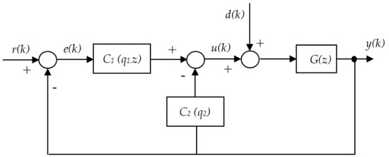
Figure 1.
Closed-loop of the feedback-type (FB)-type 2DOF (two-degrees-of-freedom) PI-P (proportional-integral/proportional) control system.
In addition, r(k), u(k), e(k), d(k) and y(k) are the reference signal, the controller output, the error between the reference and the plant output, the disturbance and the plant output, respectively. C1(q1,z) is the controller in the form of a PI controller, and C2(q2) is the controller in the form of the P controller.
where z denotes the z-operator and denotes z-transform that converts controller from a continuous-time to a discrete time. KP1, KP2 and KI represent the proportional and integral gains that are to be tuned. In the PI controller, if disturbance response is optimized, the step response tends to have an overshoot. To suppress the overshoot, the P controller is provided in the feedback loop.
Basically, Equation (2) can be decoupled in the form of a PI controller:
where .
To obtain the fictitious reference signal, the closed loop response to the step input set-point (r(k) = 1 and d(k) = 0) is considered. By performing a one-shot experiment to obtain the input/output data u0(k), y0(k), where k = 1,2,3,…,N, for initial controller parameters q1 and q2 and the reference signal r(k), the fictitious reference signal can be expressed as:
The initial controller parameters q1 and q2 are selected arbitrary, only once and relatively small.
After a one-shot experiment is performed in the closed-loop speed control of PMSM to obtain input data u0(k) and output data y0(k) as shown in Figure 2, then fictitious reference signal is formed as shown in Equation (9).
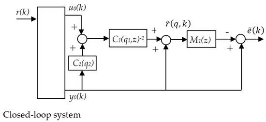
Figure 2.
2DOF PI-P fictitious reference iterative tuning (FRIT) principle.
The ideal response is obtained by multiplying fictitious reference signal with reference model M1(z), which is then the error signal , which can be calculated using:
where M1(z) is a given reference model for the step response in a discrete time, as shown in Equation (11), and:
where M1(s) is the step reference model for the step response in a continuous time and ω1 is the natural frequency (rad/s).
Using the error signal Equation (10), the performance index is minimized using:
PSO is used for FRIT optimization [11], and the Scilab program is used to program FRIT. Scilab is an open source software for scientific computation that includes hundreds of general purpose and specialized functions like MATLAB [25]. PSO is an optimization method that is based on swarm intelligence, i.e., the type of flock movement behavior that birds and fish use to find the best paths to their food. The flock of birds and the school of fish are considered as particles that are assumed to have two characteristics: position and velocity [26].
3. Disturbance Reference
This paper purposes to obtain the optimal 2DOF PI-P controller parameter for PMSM speed control, where the speed response follows the ideal response for step response and disturbance response. The step reference has been designed for the step response, as shown in Equation (11). In this section, the disturbance reference is designed as a reference for the disturbance response.
To obtain the disturbance reference, a disturbance is applied to the system. The closed loop response to a step input disturbance (d(k) = 1 and r(k) = 0) is considered.
Figure 3 shows the closed loop control system when the disturbance is applied to the system. The disturbance reference model M2(z) is the transfer function from disturbance d(k) to the controlled output y(k), and the disturbance reference model M2(z) is given based on the reference model Gr(z), which is the transfer function from reference r(k) to the output y(k), as shown in Figure 1. From Figure 1, the transfer function of Gr(z) (r(k) = 1 and d(k) = 0) can be calculated by:
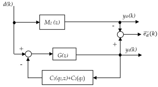
Figure 3.
2DOF closed loop disturbance system.
The transfer function from disturbance d(k) to controlled output y(k) is shown in Equation (19), where the closed loop response to a step input disturbance (d(k) = 1 and r(k) = 0) is considered.
The disturbance reference model M2(z) (22) is the same as the transfer function from disturbance d(k) to the controlled output y(k) (19).
From Equations (17) and (22), disturbance reference model M2(z) can be written by:
where C1 (q1,z) is shown in Equation (24):
Using Equations (23) and (25), the disturbance reference model M2(z) is represented as:
where:
Because the steady-state gain Gr(s) is one, it therefore follows that Gr(0) = 1 and , and thus, T(s) is given as [17]:
The disturbance reference model M2(s) in a continuous time is given:
where l is the relative degree of the controlled plant and is the natural frequency (rad/s).
When disturbance is applied to the control system (d(k) = 1 and r(k) = 0), the position of disturbance can be moved virtually to the reference position using Equations (17), (19), (22) and (23) as shown in Figure 4.
when Gr(z) is M1(z) and:
where is the reference for disturbance when the disturbance is applied to the control system and moved to the reference position. This is a virtual disturbance reference method. From Figure 4, the transfer function from the reference to the controlled output when disturbance is moved to the reference is given in Equation (37).
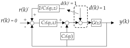
Figure 4.
Closed-loop of FB-type 2DOF PI-P control system.
This equation is the same as Equations (19) and (22).
The fictitious reference signal is presented as follows:
where:
The controller parameters can be designed for step response and disturbance response from reference r(k) to controlled output y(k) at the same time as shown below:
Step response:
r(k)→M1(z)
Disturbance response:
where r(k) is reference for step response, M1(z) is step reference model, r(k)’ is reference for disturbance when position of disturbance is moved to reference position and M2(z) is disturbance reference model.
The 2DOF PI-P controller can be designed at the same time for set-point and load-disturbance where disturbance moves to the reference when disturbance is applied to the control system and controller parameters are not designed separately.
4. PMSM Speed Control System Description
The proposed hardware control system for PMSM speed control using the FPGA is shown in Figure 5. The XILINX ARTIX-7 (XC7A100T, Digilent Inc., Pullman, WA, USA) is used to control the speed of the PMSM. The program algorithm is written in the Very High-Speed integrated circuits hardware Description Language (VHDL), which is a hardware description language that describes the behavior of an electronic circuit or system, from which the physical circuit or system can then be implemented [27]. A multiplier, an adder and subtraction are used for the calculations.
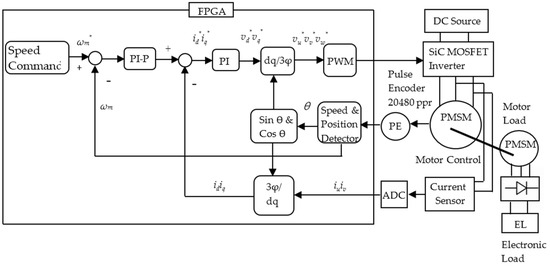
Figure 5.
Block diagram of the PMSM (permanent magnet synchronous motor) speed control.
Vector control is the PMSM control method used for variable-speed control systems. The control blocks, which include the PI-P controller as a speed controller and two PI controllers required for current control, dq (direct-axis, quadrature-axis) and inverse dq coordinate transformations, receive the speed commands. Then, a PWM pulse generator is produced for inverter switching. The speed controller is the 2DOF PI-P. An incremental pulse encoder mounted on the rotor axis of the PMSM generates a series of pulses to detect and calculate the rotor position and the motor angular speed ωm. Sensors measure the phase currents, and a 12-bit analog-to-digital (AD) converter converts these phase currents into digital values. To maximize the switching frequency, PMSM speed control is implemented using a high-performance FPGA-based digital hardware controller. The FPGA is used for torque and speed control in some cases, because fast processing operation is obtained when using its hardware processing ability.
PMSM speed control has two control loops, such as the speed control loop and minor current loop, as shown in Figure 5. The speed control loop is the control loop of speed command and measured speed. The current control loop is the control loop of plant input current iq* and q-axis current iq. The error between speed command and measured speed is amplified by the controller, then moves to plant input current iq* in the current loop. Plant input current iq* is amplified by the controller that determines the magnitude and directions of torque that causes the speed of motor ωm to be close to speed command ωm*. The magnitude of the minor current loop influences the magnitude of the speed control loop. If there are errors in the minor current loop, then there are errors in the speed control loop.
5. Experimental and Results
5.1. Experimental Setup
The experiments are performed using the proposed experimental system shown in Figure 6, and the PMSMs used for the motor control and the load (YASKAWA, Kitakyushu, Japan) in the experiment are connected via the coupling shown in Figure 7. The encoder (Heidenhain, Traunreut, Germany) is mounted on the rotor axis of the PMSM.
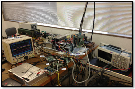
Figure 6.
Experimental apparatus.
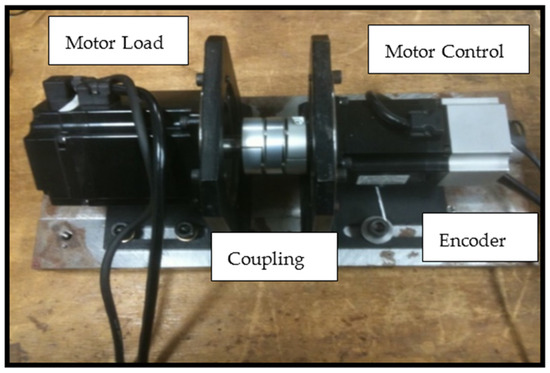
Figure 7.
Permanent magnet synchronous motor.
5.2. Results and Discussion
After the experimental apparatus has been set up, the experiment is performed to derive the input and output data, which are then processed by FRIT to tune the KP1, KP2 and KI parameters. The tuning parameters are then implemented, and the actual waveform is compared to the ideal waveform.
In the experiment, the speed command is changed from 100 min−1 to 150 min−1, and then, the step disturbance is added by applying a load to the control system when the motor speed is maintained at 150 min−1.
The model PLZ 150 W electronic load is used for motor loading and is set at 0.5 A. The clock frequency of the FPGA is set to 48 MHz, and the pulse encoder has 20,480 ppr. A PWM switching frequency of up to 100 kHz is achieved. A control frequency of up to 200 kHz is achieved, but only when the frequency of the speed detector is 50 kHz. The initial output with the step response and the disturbance response (black lines) is shown in Figure 8, and the initial input is shown in Figure 9. The speed decreases and the current increases when the motor is loaded.
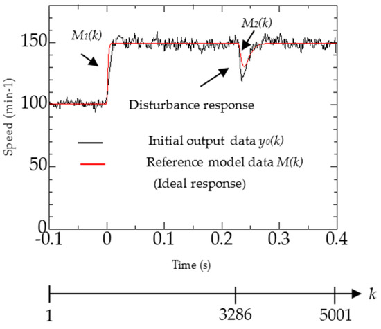
Figure 8.
Output data using the initial PI-P gain controller and reference model data.
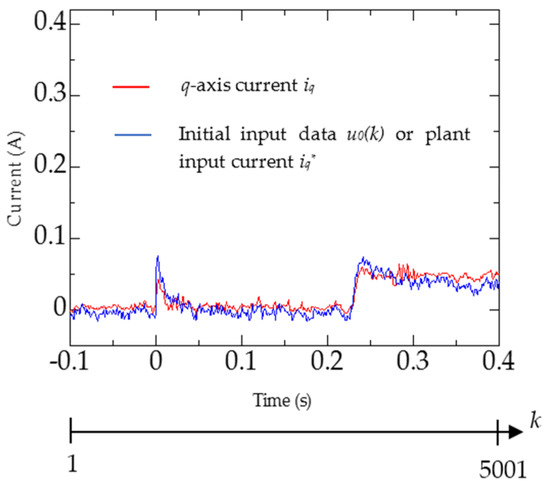
Figure 9.
Initial input data u0(k) and q-axis current iq.
The initial input (u0 (k)) and output (y0 (k)) data are taken from the one-shot experimental data from the closed loop system where the initial PI-P gain controller was implemented. The sampling time for the controller is 0.001 second. The initial PI-P gain controller parameters are as follows:
KP1 = 0.6, KI = 50, KP2 = 0.005
These parameters are chosen arbitrarily and only once the experiment is performed using the initial controller parameters. After the input and output data have been taken from the experiment, the reference model data are then formed by following the output data shown in Figure 8 (red lines). The reference model data are used for the step response and for the disturbance response.
The reference model M1(s) for the step response is represented as:
The disturbance reference model M2(s) for the disturbance response is presented as:
Natural frequency ω is the desired frequency for step reference model ω1 = 1000 rad/s and disturbance reference model ω2 = 200 rad/s.
Because the control system is a 2DOF system, the relative degree of the controlled plant is set to l = 2. The reference model M(s) is composed of the reference model for a step response M1(s), and the disturbance reference model for the disturbance response M2(s) is as shown in Figure 8.
The reference model data can be composed of:
where M(k) are the reference model data for k = 1,2,3,…,5001.
The tuning method for the proposed FRIT in the 2DOF PI-P controller is summarized as follows:
- Perform an experiment to obtain the initial input and output data (u0(k), y0(k)) in the 2DOF PI-P control system with the initial PI-P gain parameters.
- Form reference model data M(k) for the step reference model data and the disturbance model data.
- Minimize the errors between the reference M(k) and the initial output y0(k) using (13). Use PSO for FRIT optimization
The step response and the disturbance response using the initial PI-P gains are shown in Figure 8.
Figure 8 shows the output data using the initial PI-P gain controller for the step response and the disturbance response. The ideal response is compared to the output response in this figure. The output response does not follow the ideal response in this case. The disturbance response of the output is too slow to achieve the ideal response. The motor speed does not recover immediately to the steady-state condition when the motor is loaded and is affected by a disturbance. High-responsivity and optimal disturbance rejection cannot be achieved when using the initial PI-P gain controller parameters.
Figure 9 shows the q-axis current iq and the plant input current iq*. This is the minor current response using the initial PI-P gain controller. The transfer function of the minor current loop is assumed as one, and this paper mainly focuses on the speed control loop.
The errors between the reference M(k) and the initial output y0(k) are minimized using Equation (45), where the errors between the reference M(k) and y0(k) are:
The initial output data y0(k) are composed of the step response and disturbance response data; it assumed that:
The errors between the reference M(k) and y0(k) are thus:
To obtain the optimal parameters for the optimal step response and disturbance response, the performance index is minimized using:
Reference model data M(k) are composed of step reference data M1(k) and disturbance reference data M2(k). For step reference data M1(k) in the range 1 ≤ k ≤ 3286 (r(k) =1 and d(k) = 0), the performance index is evaluated from reference r(k) to controlled output y(k) using step reference model M1(z) and fictitious reference signal . For disturbance data M2(k) in the range 3287 ≤ k ≤ 5001 (r(k) = 0 and d(k) = 1), disturbance moves virtually to the reference using , so the performance index is evaluated from reference to controlled output y(k) using step reference model and fictitious reference signal , where is the disturbance reference model M2(z).
The performance index is minimized for both step response data and disturbance response data at the same time, as shown in Equation (49) in the range 1 ≤ k ≤ 5001, so optimal controller parameters can be obtained for step response and disturbance response following the step reference model and disturbance reference model.
5.3. Particle Swarm Optimization
Particle swarm optimization was developed by Kennedy and Eberhart in 1995. Kennedy and Eberhart proposed the computation technique based on the social behavior of swarms of ants, fish and birds to find the location of food. The individual of swarms, called the particle, will share the information of the location of food. The shared information is the intelligence or the knowledge of the particle. The knowledge of the particle is also the swarm knowledge and intelligence. Each individual or particle in a swarm behaves in a distributed way using its own intelligence and the collective or group intelligence of the swarm. As such, if one particle discovers a good path to food, the rest of the swarm will also be able to follow the good path instantly, even if their location is far away in the swarm [26].
The initial input (u0(k)) and output data (y0(k)) are taken from one-shot experimental data with the initial PI-P gain parameters q0 = [KP1 KP2 KI]T (q0 is a matrix of initial PI-P controller parameters where KP1, KI and KP2 are proportional, integral and proportional gains, respectively). Because the PSO algorithm is used for FRIT optimization, the data are treated as numbers of particles n, where each particle consists of PI-P gains organized in a matrix. Each particle is updated using personal best (Pbest) and global best (Gbest) values in each iteration. Pbest is the best position achieved by a particle to date, and Gbest is the best position achieved by any particle. The velocity and position of the particle are updated after the values of Pbest and Gbest have also been updated. Pbest and Gbest are updated using Equation (56) and Equation (57). The velocity is updated using Equation (58), and position is updated using Equation (62). Figure 10 shows the flowchart of the PSO algorithm for FRIT optimization.
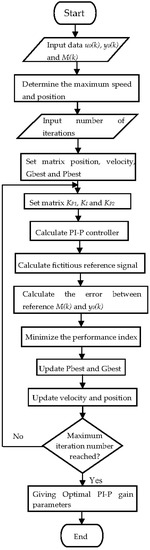
Figure 10.
Flowchart of PSO (particle swarm of optimization) algorithm for FRIT.
The algorithm of PSO for FRIT optimization is described as follows:
Step 1: input:
- -
- Input data u0(k), output data y0(k) and reference data M(k).
- -
- Determine the minimum and maximum value of speed and position of the particle.
- -
- Number of iterations.
- -
- Set matrix position, velocity, Pbest and Gbest.
Step 2: process:
For each particle k = 1,2,3,…,N in the i-th iteration,
- -
- The PI-P controller is calculated using:
- -
- The fictitious reference signal is calculated using:
- -
- The errors between the reference M(k) and y0(k) are calculated using:
- -
- The performance index is minimized using:
- -
- Pbest and Gbest are updated using:where qkp(i) and qG(i) are the personal best Pbest and the global best Gbest.
- -
- The velocity is updated using:where r1(i) and r2(i) are random functions in the range between zero and one generated by the computer, c1 and c2 are the learning rates and usually are assumed to be two and w is the inertia weight. Inertia weight w is determined using:wmax and wmin are the initial and final values of inertia weight where wmax is 0.9 and wmin is 0.4; imax is the maximum number of iterations, and i is the current iteration.
- -
- The position is updated using:where:
- update particle position (m)
- present particle position (m)
- update particle velocity (m/s)
- a time step assumed as one (s)
Step 3: output:
- -
- The optimal PI-P gain parameters are then obtained from Equation (62).
- -
- The stop iteration condition: the maximum number of iterations
- -
- The maximum number of iterations is the input of the number iterations.
The maximum number of iterations is considered to end the loop and to stop the iterations. The performance index is not considered to end the loop because there is no standard value of the performance index to obtain the optimal controller parameter. In this paper, 100 iterations are used to obtain the optimal controller parameters, because the state of controllers searched by FRIT becomes saturated if the number of iterations is more than 100 iterations.
5.4. Result of Tuned PI-P Controller
After the input, output and reference are applied to the FRIT with the initial PI-P gain parameters, the tuned controller parameters are obtained as follows:
KP1 = 0.7994, KI = 53.7175, KP2 = 0.0201
The output results when the tuned PI-P gains were applied using FRIT, as shown in Figure 11.
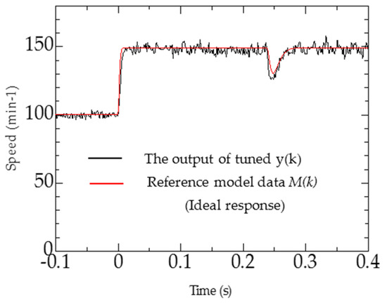
Figure 11.
Output results when tuned PI-P gains were applied using FRIT.
Figure 11 and Figure 12 show the output and input results when the tuned PI-P gains were applied, respectively. Ideal responses for both the step response and the disturbance response are shown in Figure 11. The output response follows the ideal response for both the step response and the disturbance response. The motor speed recovers immediately to the steady-state condition when the motor is loaded and is then influenced by a disturbance. High-responsivity and optimal disturbance rejection can be achieved using the tuned PI-P gain parameters. Figure 12 shows the q-axis current iq and the plant input iq*. This is the minor current response when tuned PI-P gains were applied. There are errors between q-axis current iq and plant input current iq*; therefore, there are the errors between speed response and the ideal response. Figure 13 and Figure 14 show the step responses of the initial PI-P gain controller and tuned PI-P gain controller when the time is expanded. Figure 15 and Figure 16 show the disturbance responses of the initial PI-P gain controller and the tuned PI-P gain controller when the time is expanded. High-responsivity and optimal disturbance rejection can be achieved using the 2DOF PI-P controller. The FRIT method can be used to obtain the optimal parameters for the FB PI-P controller in a 2DOF control system with the aim of achieving the ideal responses for both the step response and the disturbance response.
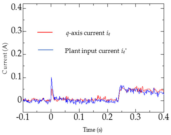
Figure 12.
Plant input current iq*, and q-axis current iq when tuned PI-P gains were applied using FRIT.
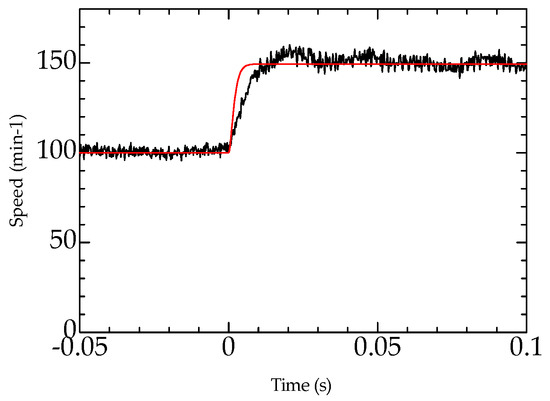
Figure 13.
Step response of the initial PI-P gain controller.
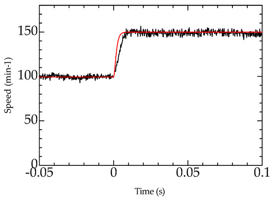
Figure 14.
Step response of the tuned PI-P gain controller.
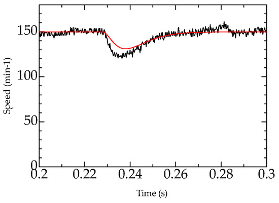
Figure 15.
Disturbance response of the initial PI-P gain controller.
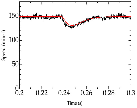
Figure 16.
Disturbance response of the tuned PI-P gain controller.
Figure 13 shows the step response of the initial PI-P controller when time is expanded.
Figure 14 shows the step response of the tuned PI-P controller when time is expanded.
Figure 15 shows the disturbance response of the initial PI-P controller when time is expanded.
Figure 16 shows the disturbance response of the tuned PI-P gain controller when time is expanded.
5.5. Result of FRIT
Figure 17 shows the value of PI-P controller parameter that is tuned by FRIT. The number of iterations is 100 iterations to obtain the controller parameter. Figure 18 is the state of fictitious reference signal after 10 iterations; Figure 19 is the state of fictitious reference signal after 30 iterations; Figure 20 is the state of fictitious reference signal after 100 iterations. Fictitious reference signal moves closer to the ideal response of each iteration.
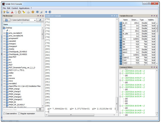
Figure 17.
The value of the PI-P controller tuned by FRIT. g1 = KP1, g2 = KI and g3 = KP2.
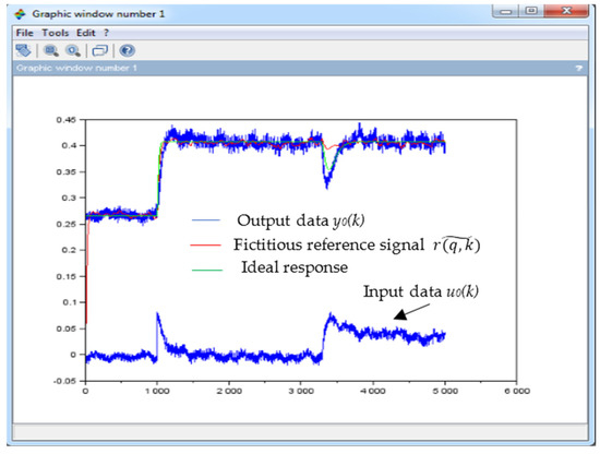
Figure 18.
The state of fictitious reference signal after 10 iterations.
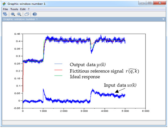
Figure 19.
The state of fictitious reference signal ) after 30 iterations.
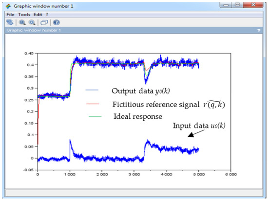
Figure 20.
The state of fictitious reference signal ) after 100 iterations.
6. Conclusions
This paper proposes a PI-P tuning method for the speed control of a PMSM using an FPGA for a high-frequency SiC MOSFET inverter and using the FRIT method in a 2DOF control system. There has been no research available on tuning the 2DOF PI-P controller using the FRIT method for speed control of a PMSM using FPGA for a high-frequency SiC MOSFET inverter. FRIT is applicable to the tuning of the controller parameters based on the input and output data obtained from one-shot experimental data. This paper proposes tuning of the controller parameters using a step reference and a disturbance reference in the FRIT method, so that optimal parameters can be achieved when a disturbance is applied to the control system.
Optimal 2DOF PI-P controller parameters can be achieved, where the output response follows the ideal response for both the step response and the disturbance response, when using the proposed method.
Switching frequencies of up to 100 kHz can be achieved using the SiC MOSFET, so that the motor speed can recover immediately when the motor is loaded and is then affected by a disturbance. The output response follows the ideal response characteristics for the step response and the disturbance response. High-responsivity and optimal disturbance rejection can be achieved using the proposed 2DOF PI-P control system.
There is error in the minor current loop, so there is error between the ideal response and the speed response. Further research is how to design a method to minimize the error of the minor current loop close to zero so that the speed response is very close to the ideal response.
Author Contributions
Charles Ronald Harahap and Tsuyoshi Hanamoto conceived of and designed the experiments. Charles Ronald Harahap performed the experiments. Charles Ronald Harahap and Tsuyoshi Hanamoto analyzed the data. Charles Ronald Harahap and Tsuyoshi Hanamoto contributed to the analysis tools. Charles Ronald Harahap wrote the paper.
Conflicts of Interest
The authors declare no conflict of interest.
References
- Lai, R.; Wang, L.; Sabate, J.; Elasser, A.; Stevanovic, L. High-voltage high- frequency inverter using 3.3 kV SiC MOSFETs. In Proceedings of the 15th International Power Electronics and Motion Control Conference, Novi Sad, Serbia, 4–6 September 2012; pp. 1–5.
- Johnson, C.M. Comparison of silicon and silicon carbide semiconductors for a 10 kV switching application. In Proceedings of the 35th Annual IEEE Power Electronics Specialists Conference, Aachen, Germany, 20–25 June 2004; pp. 572–578.
- Shen, M.; Krishhamurthy, S. Simplified loss analysis for high speed SiC MOSFET inverter. In Proceedings of the 2012 Twenty-Seventh Annual IEEE Applied Power Electronics Conference and Exposition, Orlando, FL, USA, 5–9 February 2012; pp. 1682–1687.
- Shen, M.; Krishhamurthy, S.; Muldhokar, M. Design and performance of a high frequency silicon carbide inverter. In Proceedings of the IEEE Energy Conversion Congress and Exposition, Phoenix, AZ, USA, 17–22 September 2011; pp. 2044–2049.
- Shirabe, A.K.; Swamy, M.; Kang, J.K.; Hisatsune, M.; Wu, Y.; Kebort, D.; Honea, J. Advantages of high frequency PWM in AC motor drive applications. In Proceedings of the IEEE Energy Conversion Congress and Exposition, Releigh, NC, USA, 15–20 September 2012; pp. 2977–2984.
- Araki, M.; Taguschi, H. Two-degree-of-freedom PID controllers, tutorial paper. Int. J. Control Autom. Syst. 2003, 12, 401–411. [Google Scholar]
- Harahap, C.R.; Saito, R.; Yamada, H.; Hanamoto, T. Speed control of permanent magnet synchronous motor using FPGA for high frequency SiC MOSFET inverter. J. Eng. Sci. Technol. 2014, 11–20. [Google Scholar]
- Soma, S.; Kaneko, O.; Fujii, T. A new approach to parameter tuning of controllers by using one-shot experimental data—A Proposal of Fictititous Reference Iterative Tuning. Trans. Inst. Syst. Control Inf. Eng. 2004, 17, 528–536. [Google Scholar]
- Soma, S.; Kaneko, O.; Fujii, T. A new method of a controller parameter tuning based on input-output data – Fictitious Reference Iterative Tuning. In Proceedings of the 2nd IFAC workshop on Adaptation and Learning in Control and Signal Processing (ALCOSP), Yokohama, Japan, 30 August–1 September 2004.
- Wakasa, Y.; Tanaka, K.; Nishimura, Y. Online controller tuning via FRIT and recursive least-squares. In Proceedings of the IFAC Conference on Advances in PID Control, Brescia, Italy, 28–30 March 2012; Volume 2, pp. 76–80.
- Azuma, T.; Watanabe, S. A design of PID controllers using FRIT-PSO. In Proceedings of the 8th International Conference of Sensing Technology, Liverpool, UK, 2–4 September 2014; pp. 459–464.
- Kaneko, O.; Soma, S.; Fuji, T. A Fictitious Reference Iterative Tuning (FRIT) in the two degree of freedom control scheme and its application to closed loop system identification. In Proceedings of the 16th Triennial World Congress, Prague, Czech Republic, 4–8 July 2005.
- Kaneko, O.; Yamashina, Y.; Yamamoto, S. Fictitious reference tuning for the optimal parameter of a feedforward controller in the two degree of freedom control system. In Proceedings of the IEEE International Conference on Control Applications, Yokohama, Japan, 8–10 September 2010.
- Kaneko, O.; Yamashina, Y.; Yamamoto, S. Fictitious reference tuning of the feed-forward controller in a two-degree-of-freedom control system. SICE J. Control Meas. Syst. Integr. 2011, 4, 55–62. [Google Scholar] [CrossRef]
- Kaneko, O.; Souma, S.; Fujii, T. Fictitious reference iterative tuning in the two-degree-of-freedom control scheme and its application to a facile closed loop system identification. Trans. Soc. Instrum. Control Eng. 2006, 42, 17–25. [Google Scholar] [CrossRef]
- Harahap, C.R.; Hanamoto, T. FRIT based PI tuning for speed control of PMSM using FPGA for high frequency SiC MOSFET Inverter. In Proceedings of the 4th International Conference on Informatics, Electronics, & Vision, Kitakyushu, Japan, 15–18 June 2015.
- Masuda, S. A direct PID gains tuning method for DC Motor control using an input-output data generated by disturbance response. In Proceedings of the IEEE International Conference on Control Applications (CCA), Denver, CO, USA, 28–30 September 2011; pp. 724–729.
- Hjalmarsson, H. Iterative Feedback Tuning-an overview. Int. J. Adapt. Control Signal. Process. 2002, 16, 373–395. [Google Scholar] [CrossRef]
- Campi, M.C.; Savaresi, S.M. Direct Nonlinear Control Design: The Virtual Reference Feedback Tuning (VRFT) Approach. IEEE Trans. Autom. Control 2006, 51, 14–27. [Google Scholar] [CrossRef]
- Lecchini, A.; Campi, M.C.; Savaresi, S.M. Virtual reference feedback tuning for two-degree-of-freedom controllers. Int. J. Adaptive Control Signal. Process. 2002, 16, 355–371. [Google Scholar] [CrossRef]
- Rojas, J.D.; Vilanova, R. Feedforward based two degree of freedom formulation of the virtual reference feedback tuning approach. In Proceedings of the European Control Conference, Budapest, Hungary, 23–26 August 2009; pp. 1800–1805.
- Gazdos, F.; Dostal, P. Direct controller design and iterative tuning applied to the coupled drives apparatus. J. Electr. Eng. 2009, 60, 106–111. [Google Scholar]
- Liaw, C.M. Design of a two-degree-of-freedom controller for motor drives. IEEE Trans. Autom. Control 1992, 37, 1215–1220. [Google Scholar] [CrossRef]
- Hanamoto, T.; Deriha, M.; Ikeda, H.; Tsuji, T. Digital hardware circuit using FPGA for speed control system of permanent magnet synchronous motor. In Proceedings of 18th International Conference on Electrical Machines, Vilamoura, Portugal, 6–9 September 2008; pp. 1–5.
- Campbell, S.L.; Chancelier, J.-P.; Nikoukhah, R. Modeling and Simulation in Scilab./Scicos; Springer Science + Business Media: New york, NY, USA, 2006. [Google Scholar]
- Rao, S.S. Engineering Optimization, Theory and Practice, 3rd ed.; John Wiley & Sons, Inc., Wiley Eastern Limited, publishers and New Age International Publishers, Ltd.: New Jersey, NJ, USA, 2009. [Google Scholar]
- Pedroni, V.A. Circuit Design with VHDL; MIT Press: Cambridge, MA, USA, 2004. [Google Scholar]
© 2016 by the authors; licensee MDPI, Basel, Switzerland. This article is an open access article distributed under the terms and conditions of the Creative Commons Attribution (CC-BY) license (http://creativecommons.org/licenses/by/4.0/).