Multi-Dimensional Detection Capability Analysis of Surface and Surface-to-Tunnel Transient Electromagnetic Methods Based on the Spectral Element Method

Abstract

The transient electromagnetic (TEM) method is a key detection and monitoring technology for safe coal-mine production. Surface TEM depth penetration is limited by real geological conditions and transmitter–receiver hardware performance. Compared with the surface TEM method, the tunnel TEM method can enhance the depth of exploration to some extent, but it is constrained by the limited working space of the roadway, which makes it difficult to perform the area-wide and multi-line data acquisition, and thus the lateral detection resolution is directly compromised. Consequently, either surface or tunnel TEM alone suffers inherent limitations. The multidimensional surface and surface-to-tunnel TEM method employs a single large-loop transmitter and records electromagnetic (EM) signals both on the surface and in the tunnel, enabling joint data interpretation. The joint TEM observation method effectively addresses the limitations by using a single observation mode, with the goal of achieving high-precision detection. To investigate the detection capabilities of the joint surface and surface-to-tunnel TEM method, we propose a three-dimensional (3D) joint surface and surface-to-tunnel TEM forward modeling method based on the spectral element method (SEM). The SEM, using high-order vector basis functions, enables high-precision modeling of TEM responses with complex geo-electric earth models. The accuracy of the SEM is validated through comparisons with one-dimensional (1D) TEM semi-analytical solutions. To further reveal TEM response characteristics and multi-dimensional resolution under joint surface and tunnel detection modes, we construct several typical 3D geo-electric earth models and apply the SEM algorithm to simulate the TEM responses. We systematically analyze the horizontal and vertical resolution of 3D earth model targets at different decay times. The numerical results demonstrate that surface multi-line TEM surveying can accurately delineate the lateral extent of the target body, while vertical in-tunnel measurements are crucial for identifying the top and bottom interfaces of geological targets adjacent to the tunnel. Finally, the theoretical modeling results demonstrate that compared to individual TEM methods, the multi-dimensional joint surface and tunnel TEM observation yields superior target spatial information and markedly improves TEM detection efficacy under complex conditions. The 3D TEM forward modeling based on the SEM provides the theoretical foundation for subsequent 3D inversion and interpretation of surface-to-surface and surface-to-tunnel joint TEM data.

1. Introduction

Most coal mining operations adopt underground extraction methods, which face challenges such as complex geological conditions, hidden water hazards in fractured zones, and a heightened risk of collapse-related accidents. Therefore, it is critical to develop effective mining geophysical techniques to ensure the safety and efficiency of coal mining. Typical coalfield and mine geophysical techniques primarily include seismic exploration [1,2,3], the direct current resistivity (DC) method [4,5,6,7,8,9,10], and the transient electromagnetic (TEM) method [11,12,13,14,15,16,17]. The seismic exploration method is highly effective for coal seam delineation and structural mapping, but has significant limitations in determining the hydraulic conductivity and water-bearing properties of hidden water-related hazards such as fractured zones and aquifers. The DC method, despite its strong anti-interference capability and good penetration performance, is hampered in practical applications by issues such as low operational efficiency, high labor intensity, and difficulties with underground communication. Daniel et al. investigated the feasibility of detecting abandoned mine goafs using coal seam channel waves [3]. Li et al. reviewed the applications, technical issues, and development trends of the DC method for water-inrush detection and monitoring in coal-mine roadways and other tunnels [8].

Electromagnetic (EM) exploration methods are based on resistivity contrasts as the target physical property. These methods play a crucial role in coalfield geology and hydrogeological exploration. Notably, coalfield strata tend to exhibit a near-horizontal, layered structure. This favors the effective identification of low-resistivity anomalies using large-loop TEM surveys. The application of the surface TEM in coal mines began with the detection of water-rich sandstone zones in roadway roofs [11]. Subsequently, Yue et al. summarized TEM applications in underground mines and reviewed the historical development of electrical exploration methods used for advance detection in tunnels and working faces of Chinese coal mines, identifying key technologies, existing problems, and future directions [12,13]. Xue et al. summarized future breakthrough directions for TEM applications in the coal industry and demonstrated the effectiveness of the TEM method in this field [14]. Xue et al. proposed a full-waveform inversion method for TEM data based on the virtual wave field to improve the depth resolution and parameter estimation accuracy of subsurface resistivity imaging [15]. Li et al. proposed a TEM data inversion method constrained by seismic information to enhance the accuracy of detecting water-bearing zones in coal-mine roofs within the Ordos Basin [17].

Additionally, underground (such as borehole and tunnel) TEM surveys in mines and tunnels have been widely used for roadway and subsurface detection due to their flexibility, operational convenience, and high sensitivity to low-resistivity anomalies [18,19,20,21,22,23,24,25]. Yue et al. established a boundary element-based EM forward model for subsurface current-field simulation, incorporating a “roadway influence factor function” to quantitatively analyze roadway-induced perturbations in current-field distribution [18]. Li et al. applied the TEM to hydrogeological investigation, using EM responses at different time channels to characterize the geo-electric properties of media at varying depths [19]. This method successfully delineated the three-dimensional (3D) spatial distribution of water-inrush channels and water-enriched zones within the surveyed region. Jiang et al. experimentally validated the applicability of the multi-TEM method for predicting water-bearing anomalies ahead of advancing roadways [20]. Jiang developed theoretical frameworks for whole-space magnetic dipole excitation perpendicular and parallel to bedding planes, based on the stratified geo-electric characteristics of coal-bearing formations and underground TEM forward detection principles [21].

When water-rich geological bodies such as water-bearing collapse columns, faults, or goaf water exist in the roofs or floor strata of coal seams, their electrical conductivity is significantly enhanced. This results in a distinct electrical contrast with the surrounding rocks, a phenomenon that creates a favorable physical basis for EM methods. Although the integrated application of the TEM with seismic exploration has demonstrated remarkable effectiveness—particularly in detecting hazardous geological features like goafs and collapse columns—the accuracy and reliability of conventional TEM configurations remain inadequate in complex coal mining environments. This limitation can be observed in both surface TEM systems employing large-loop transmitters and underground TEM systems utilizing short-offset configurations, primarily stemming from two aspects: (1) the surface TEM is significantly affected by the shielding effect of shallow low-resistivity aquifers, which attenuates the effective detection depth and hampers accurate acquisition of mid-to deep-level geological information; and (2) mine-tunnel TEM configurations acquire data directly within roadways, effectively circumventing interference from low-resistivity surface layers and achieving enhanced proximity to target geological bodies, which yields stronger secondary-field responses. However, confined by the narrow space of underground roadways, the transmitting coil is usually designed as a small multi-turn loop, resulting in a low magnetic moment and limited detection range—typically within 100 m. Moreover, a significant blind zone exists near the probe. Low construction efficiency and high labor intensity further restrict its capability to detect distant hazards ahead of the working face and deep-seated hazards in the roof and floor strata. To enhance the applicability and accuracy of the TEM in complex mining environments, it is imperative to systematically integrate multi-parameter acquisition, multi-component data fusion, and multi-method collaborative inversion. Such technical integration can facilitate substantial improvements in both detection precision and interpretation reliability.

The surface and surface-to-tunnel EM is an emerging geophysical technique [26]. It integrates a loop transmitter source laid out on the earth’s surface with multi-receivers deployed on the surface, in boreholes, or in tunnels. This configuration enables multi-dimensional data acquisition in both lateral and vertical directions, significantly enhancing spatial sampling capabilities. This method includes the surface-to-surface TEM, surface-to-borehole TEM, and surface-to-tunnel TEM modes. Its technical advantages are as follows: (1) The transmitter is free from underground operational constraints and can operate at high power; receivers can be deployed over extensive surface areas, providing high lateral resolution for the acquired signals. (2) Borehole and tunnel receivers can be placed close to or within the target, markedly improving the signal-to-noise ratio. Li carried out an integrated interpretation of surface and underground TEM data, leading to enhanced detection accuracy for concealed water-inrush hazards in coal mines [26]. However, current research on the surface-to-tunnel TEM and its data interpretation remains limited. In particular, the data processing and interpretation for combined surface-to-tunnel TEM observations primarily rely on one-dimensional (1D) EM forward modeling and inversion. This approach has certain limitations when considering the complexity of actual geological conditions. Since high-precision forward modeling is fundamental to 3D inversion, it is important to conduct corresponding forward and inversion studies based on 3D geo-electric earth models.

In recent years, advancements in numerical methods and their computational efficiency have led to the gradual maturation of 3D EM forward modeling technology. Conventional 3D EM forward modeling schemes for the TEM include the Integral Equation Method (IEM) [27,28], Finite Difference Method (FDM) [29,30], Finite Element Method (FEM) [31,32], and Finite Volume Method (FVM) [33,34]. Michael et al. introduced a novel IEM scheme for 3D electromagnetic modeling of complex targets embedded in an in-homogeneous background conductivity (IBC) [35]. Chen et al. used the IEM to simulate the response of the tunnel–borehole TEM configuration under full-space conditions [36]. With the IEM, the mesh is discretized only inside the anomalous body, eliminating the need for grid division of the entire computational domain, which significantly reduces the number of unknowns and therefore the overall computational load. This feature enables the IEM to produce a relatively small linear system, yielding both fast computation and efficient solutions. However, the IEM’s matrix is dense and asymmetric; the extremely refined meshes required for complex models rapidly consume memory and impair its adaptability to intricate geometries. Yue et al. derived a 3D finite-difference time-domain (FDTD) algorithm for full-space mine TEM fields and implemented Mur’s absorbing boundary conditions, markedly reducing the computational load [37]. Sun et al. employed the FDTD method to investigate TEM response curves and the disturbance caused by a large tunnel boring machine in tunnel ahead-prospecting, and, based on linear field superposition, proposed a “subtraction” correction technique [38]. Chang et al. used the FDTD method to simulate the TEM responses of quarries of variable shape and filled with water at different locations [39]. The FDM partitions the domain into structured hexahedral cells, assigning degrees of freedom to nodes, edges, or faces as needed. However, the rigid grid structure limits its accuracy for complicated models, introducing significant geometric errors and pronounced trapezoidal distortion. The FEM offers higher accuracy than the FDM. Xiong et al. presented a 2D FEM forward algorithm for TEM modeling in configurations with piece wise uniform conductivity [40]. Wang et al. proposed a mixed-element finite-element method for 3D DC-resistivity forward modeling and investigated how borehole parameters influence apparent-resistivity data acquired with borehole-to-surface and surface-to-borehole arrays [32]. The FEM offers greater flexibility in mesh discretization, as it can utilize both hexahedral elements and unstructured tetrahedral elements, making it better suited for modeling complex geological structures. However, capturing fine model details typically demands a large number of elements, resulting in an enormous and structurally complex coefficient matrix and high memory requirements, which can drastically reduce overall solution efficiency. The FVM combines features of both the FEM and FDM, drawing on each of their advantages. Haber et al. proposed a universal 3D time-domain EM inversion algorithm that integrates the FVM with an improved Gauss–Newton inversion technique, applicable to any electromagnetic field data measured on the surface or in boreholes [41]. The FVM can therefore manage complex models; however, it inevitably also inherits the shared drawbacks of both the FEM and the FDM, such as a difficulty in balancing accuracy and efficiency.

To reduce the accuracy dependence of forward responses on physical mesh discretization, the spectral element method (SEM), a high-order vector basis-function approach for solving partial differential equations, has increasingly been applied to geophysical electromagnetic modeling [42,43,44,45,46]. Frequency-domain airborne EM forward modeling using the SEM based on regular grids has recently been successfully implemented. Yin et al. and Huang et al. demonstrated that the SEM can be used to simulate airborne EM responses for simple, regular geological bodies [42,43]. They also confirmed that combining high-order spectral element basis functions with relatively coarse grids enables high-precision forward modeling. Huang et al. developed 3D forward modeling of airborne electromagnetic data for complex geo-electric models using the SEM, laying the foundation for high-precision and rapid inversion [44]. Huang et al. demonstrated that under comparable conditions, the SEM achieves higher accuracy than the conventional FEM [46]. The method first employs the Galerkin residual method to derive the weak form of the partial differential equations. It integrates principles from both spectral methods and the FEM, specifically adopting high-order orthogonal basis functions with spectral convergence from spectral methods as trial and basis functions, while utilizing the numerical approach of the FEM. The computational domain is discretized using regular or irregular physical grids. The coefficient matrix corresponding to the spectral element basis functions is then assembled, and field values at the discrete grid points are obtained by solving the resulting large linear system. For field values at arbitrary positions, interpolation based on the SEM basis functions within the relevant grid element is performed. Therefore, the SEM combines the advantages of spectral methods’ high accuracy and the FEM’s flexible mesh discretization capability for arbitrary grids. By using high-order basis functions with spectral convergence, such as Gauss–Lobatto–Chebyshev (GLC) or Gauss–Lobatto–Legendre (GLL) orthogonal polynomials, this method achieves high-precision simulations on relatively coarse grids. This approach reduces the dependence of simulation results on grid resolution and enables accurate representation of field variations within any discrete element through high-order interpolation functions. The SEM has been widely used in computational simulations across multiple disciplines, including fluid dynamics, EM wave-guide analysis and microwave engineering, and exploration seismology [47,48,49]. In contrast, the implementation of SEM forward and inverse modeling for surface-to-tunnel configurations in current geophysical research remains relatively underdeveloped. To date, only a limited number of studies have demonstrated its applicability in this domain, notably including land, airborne and marine EM forward modeling [50,51,52].

We present a 3D forward modeling method for the surface and surface-to-tunnel TEM using the SEM. Initially, the forward modeling theory is established to calculate both surface and surface-to-tunnel TEM responses with regular hexahedral spectral elements. Subsequently, the accuracy of hexahedral SEM discretization is validated through comparative error analysis against semi-analytical 1D solutions, while the dependence of modeling precision on polynomial order is systematically investigated for both surface and surface-to-tunnel TEM configurations. Finally, the proposed algorithm is applied to model the TEM responses of various complex 3D anomalous bodies with both surface and surface-to-tunnel TEM modes, we analyze their characteristics and evaluate the horizontal and vertical resolution of combined surface and surface-to-tunnel detection, and provide a summary of the joint surface and surface-to-tunnel TEM observation and detection effects of typical geo-electric models. This study provides valuable theoretical insights for practically applying this method.

2. 3D SEM Forward Method of Surface-to-Tunnel TEM

Starting from the time-domain Maxwell equations:

$$\begin{array}{l}\nabla \times \mathbf{E}=-{\displaystyle \frac{\partial \mathbf{B}}{\partial t}}\\ \nabla \times \mathbf{H}=\mathbf{j}+{\displaystyle \frac{\partial \mathbf{D}}{\partial t}}\\ \nabla \cdot \mathbf{B}=0\\ \nabla \cdot \mathbf{D}=q\end{array}.$$

(1)

The electric-field diffusion equation can be derived as

$$\nabla \times \left({\mu }^{-1}\nabla \times \mathbf{E}\right)+\sigma \cdot {\displaystyle \frac{\partial \mathbf{E}}{\partial t}}=-{\displaystyle \frac{\partial \mathbf{J}}{\partial t}}.$$

(2)

By discretizing the model space with an arbitrary hexahedral mesh, the electric field within any hexahedral element at a given time channel t can be expressed using SEM basis functions as follows:

$$\mathbf{E}\left(x,y,z\right)={\displaystyle \sum _{i=1}^{N_e}{\mathbf{E}}_i {\tilde{\mathbf{\Phi }}}_i\left(x,y,z\right)}.$$

(3)

where Nₑ is the number of SEM basis functions in a single element. Considering that the 3D spectral element basis functions are generally defined by orthogonal polynomials, the domain is $\left[-1,1\right]\times \left[-1,1\right]\times \left[-1,1\right]$. Using the Jacobian matrix Γ, the mapping between the basis functions of an arbitrary hexahedral element in the physical domain and those of the standard reference element is established as

$$\tilde{\mathbf{\Phi }}\left(x,y,z\right)={\Gamma }^{-1}\mathbf{\Phi }\left(\xi ,\eta ,\zeta \right).$$

(4)

The SEM basis functions on the reference element are constructed using GLL polynomials $\mathbf{\Phi }\left(\xi ,\eta ,\zeta \right)$:

$$\mathbf{\Phi }\left(\xi ,\eta ,\zeta \right)=\left[\begin{array}{c}{\phi }^{(N-1)}\left(\xi \right){\phi }^{(N)}\left(\eta \right){\phi }^{(N)}\left(\zeta \right)\\ {\phi }^{(N)}\left(\xi \right){\phi }^{(N-1)}\left(\eta \right){\phi }^{(N)}\left(\zeta \right)\\ {\phi }^{(N)}\left(\xi \right){\phi }^{(N)}\left(\eta \right){\phi }^{(N-1)}\left(\zeta \right)\end{array}\right].$$

(5)

where N denotes the polynomial order of the basis functions, $\xi$, $\eta$, and $\zeta$ indicate the three orthogonal directions of the reference domain, and $\phi$ is the 1D GLL polynomial. The entire computational domain is discretized with elements that all adopt Nth-order basis functions, so inter-element continuity is automatically enforced.

Based on the form of the governing equations presented earlier, the corresponding residual R can be defined. Through the Galerkin weighted residual method and by utilizing the dyadic Green’s first theorem, together with the boundary conditions, R can be expressed as

$$\begin{array}{l}{\displaystyle \underset{{\Omega }_{\mathit{e}}}{\int }{\left[\left(\nabla \times \mathbf{\nu }\right)\cdot \left(\nabla \times {\mathbf{E}}^{\mathrm{s}}\right)\right]}_{\mathit{i}}\mathit{d}}{\Omega }_{\mathit{e}}+\mu {\displaystyle \underset{{\Omega }_{\mathit{e}}}{\int }{\left[\mathbf{\nu }\cdot \mathit{\sigma }\cdot \frac{\partial E^{\mathrm{s}}}{\partial \mathit{t}}\right]}_{\mathit{i}}\mathit{d}}{\Omega }_{\mathit{e}}\\ +\mu {\displaystyle \underset{{\Omega }_{\mathit{e}}}{\int }{\left[\mathbf{\nu }\cdot \left(\sigma -{\sigma }^{\mathrm{p}}\right)\cdot \frac{\partial E^{\mathrm{p}}}{\partial \mathit{t}}\right]}_{\mathit{i}}\mathit{d}}{\Omega }_{\mathit{e}}=0\end{array}.$$

(6)

where v is the weight function.

In this paper, the spectral element method is employed to solve boundary value problems. Since the computational domain is discretized using regular hexahedral elements, the vector basis functions are only tangential to the x, y, and z axes, designated as ${\tilde{\mathbf{\Phi }}}_j^x\left(x,y,z\right)$, ${\tilde{\mathbf{\Phi }}}_j^y\left(x,y,z\right)$, and ${ \tilde{\mathbf{\Phi }}}_j^z\left(x,y,z\right)$, respectively. Thus, the time-domain electric field in any element can be interpolated as

$$\begin{array}{l}E={\displaystyle \sum _{t=0}^{N_z}{\displaystyle \sum _{s=0}^{N_y}{\displaystyle \sum _{r=0}^{N_{x-1}}{E}_j^x{ \tilde{\mathbf{\Phi }}}_j^x\left(x,y,z\right)}}}+{\displaystyle \sum _{t=0}^{N_z}{\displaystyle \sum _{s=0}^{N_{y-1}}{\displaystyle \sum _{r=0}^{N_x}{E}_j^y{ \tilde{\mathbf{\Phi }}}_j^y\left(x,y,z\right)}}}\\ +{\displaystyle \sum _{t=0}^{N_{z-1}}{\displaystyle \sum _{s=0}^{N_y}{\displaystyle \sum _{r=0}^{N_x}{E}_j^z{ \tilde{\mathbf{\Phi }}}_j^z\left(x,y,z\right)}}}={\displaystyle \sum _{j=1}^M{E}_j {\tilde{\mathbf{\Phi }}}_j\left(x,y,z\right)}\end{array}.$$

(7)

Substituting Equation (7) into Equation (6) and replacing v with Φ yields

$$\begin{array}{l}\left[{\displaystyle \sum _{j=1}^M{E}_j^s}{\displaystyle \underset{{\Omega }_e}{\int }{\left(\nabla \times {\tilde{\Phi }}_i\right)}^{\mathrm{T}}\cdot \left(\nabla \times {\tilde{\Phi }}_j\right)d}{\Omega }_e+\mu \sigma {\displaystyle \sum _{j=1}^M\frac{\partial E_j^s}{\partial \mathrm{t}}}{\displaystyle \underset{{\Omega }_e}{\int }{\left({\tilde{\Phi }}_i\right)}^{\mathrm{T}}\cdot {\tilde{\Phi }}_{j}d}{\Omega }_e\right.\\ {\left.+\mu \left(\sigma -{\sigma }^{\mathrm{p}}\right){\displaystyle \sum _{j=1}^M\frac{\partial E_j^p}{\partial \mathrm{t}}}{\displaystyle \underset{{\Omega }_e}{\int }{\left({\tilde{\Phi }}_i\right)}^{\mathrm{T}}\cdot {\tilde{\Phi }}_{j}d}{\Omega }_e\right]}_i=0\end{array}.$$

(8)

To compute the element matrices, the mesh is mapped from the physical domain to the reference domain, where Equation (8) can be transformed into an integral form according to Equation (4):

$${\left[\begin{array}{l}{\displaystyle \sum _{j=1}^M{E}_j^s{\displaystyle {\int }_{-1}^1{\displaystyle {\int }_{-1}^1{\displaystyle {\int }_{-1}^1{\left(\nabla \times {\mathbf{\Phi }}_i\right)}^T\cdot \mathbf{J}\cdot {\mathbf{J}}^T\cdot \left(\nabla \times {\mathbf{\Phi }}_j\right)\frac{1}{\left|\mathbf{J}\right|}}d\xi }d\eta }d\zeta }\\ +\mu \sigma {\displaystyle \sum _{j=1}^M\frac{\partial E_j^s}{\partial t}{\displaystyle {\int }_{-1}^1{\displaystyle {\int }_{-1}^1{\displaystyle {\int }_{-1}^1{\left({\mathbf{\Phi }}_i\right)}^T\cdot {\mathbf{J}}^{-T}\cdot {\mathbf{J}}^{-1}\cdot {\mathbf{\Phi }}_j\left|\mathbf{J}\right|}d\xi }d\eta }d\zeta }\\ +\mu \left(\sigma -{\sigma }^{\mathrm{p}}\right){\displaystyle \sum _{j=1}^M\frac{\partial E_j^p}{\partial t}{\displaystyle {\int }_{-1}^1{\displaystyle {\int }_{-1}^1{\displaystyle {\int }_{-1}^1{\left({\mathbf{\Phi }}_i\right)}^T\cdot {\mathbf{J}}^{-T}\cdot {\mathbf{J}}^{-1}\cdot {\mathbf{\Phi }}_j\left|\mathbf{J}\right|}d\xi }d\eta }d\zeta }\end{array}\right]}_i=0.$$

(9)

where M and S denote the global mass and stiffness matrices, respectively, and J(t) is the discrete current-source vector. These can be rewritten via the mapping relationship into integral form in the reference coordinate system as

$$\begin{array}{l}S={\displaystyle {\int }_{-1}^1{\displaystyle {\int }_{-1}^1{\displaystyle {\int }_{-1}^1{\left(\nabla \times {\mathbf{\Phi }}_{\mathit{i}}\right)}^{\mathit{T}}\cdot \mathbf{J}\cdot {\mathbf{J}}^{\mathit{T}}\cdot \left(\nabla \times {\mathbf{\Phi }}_{\mathit{j}}\right)\frac{1}{\left|\mathbf{J}\right|}}\mathit{d}\xi }\mathit{d}\eta }\mathit{d}\zeta \\ M=\mu \sigma {\displaystyle {\int }_{-1}^1{\displaystyle {\int }_{-1}^1{\displaystyle {\int }_{-1}^1{\left({\mathbf{\Phi }}_{\mathit{i}}\right)}^{\mathit{T}}\cdot {\mathbf{J}}^{-\mathit{T}}\cdot {\mathbf{J}}^{-1}\cdot {\mathbf{\Phi }}_{\mathit{j}}\left|\mathbf{J}\right|}\mathit{d}\xi }\mathit{d}\eta }\mathit{d}\zeta \end{array}.$$

(10)

Then, Equation (9) can be rewritten as

$$M{\displaystyle \frac{\partial E}{\partial \mathrm{t}}}+SE+=\mathbf{J}\left(\mathit{t}\right).$$

(11)

To obtain an accurate time response at any arbitrary time channel t, we adopt the unconditionally stable second-order backward Euler difference scheme for temporal discretization.

$$f^{\prime }(t)={\displaystyle \frac{df(t)}{dt}}={\displaystyle \frac{1}{2\Delta t}}[3f(t)-4f(t-\Delta t)+f(t-2)\Delta t].$$

(12)

According to the attenuation characteristics of the EM field, the time-step size $\Delta t$ is progressively increased. This yields the discrete equation for any desired time gate:

$$\left(3\mathbf{M}+2\Delta t\mathbf{S}\right){\mathbf{E}}^{k+2}\left(t\right)=\mathbf{M}\left(4{\mathbf{E}}^{k+1}\left(t\right)-{\mathbf{E}}^k\left(t\right)\right)-2\Delta t{\mathbf{J}}^{k+2}\left(t\right).$$

(13)

Equation (13) can be expressed as a large-scale linear system:

$$\mathbf{KE}=\mathbf{b}.$$

(14)

where K is the left-hand-side coefficient matrix, b is the right-hand-side coefficient matrix, and E is the unknown electric field column vector.

According to Faraday’s law of induction, the TEM response dBz/dt can be written as

$${\displaystyle \frac{\partial B_z}{\partial t}}=-({\displaystyle \frac{\partial E_y}{\partial x}}-{\displaystyle \frac{\partial E_x}{\partial y}})$$

(15)

The concrete expression for dBz/dt is obtained by further discretizing the spectral element interpolation equation.

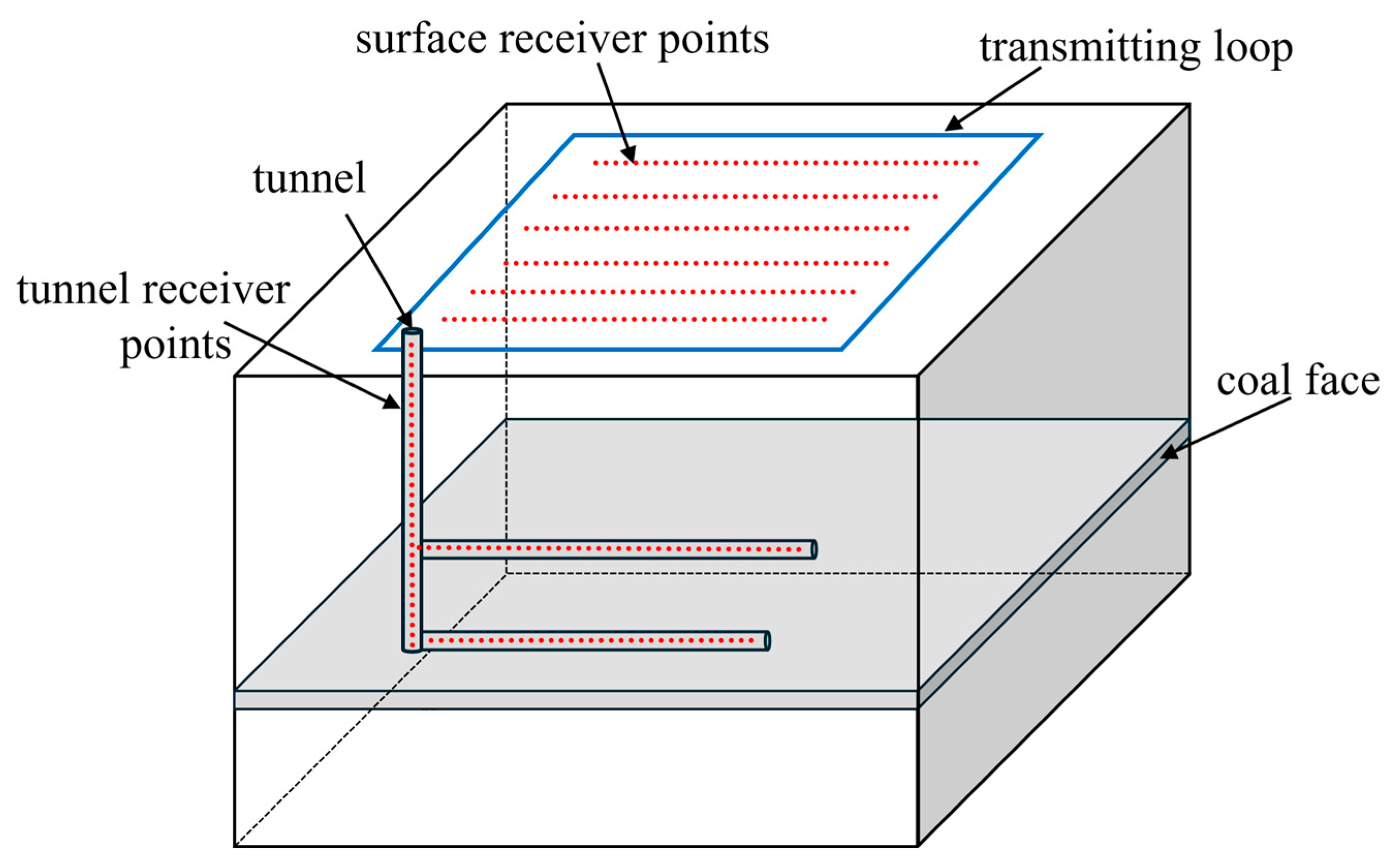
The layout of the surface-to-surface and surface-to-tunnel TEM configurations is illustrated in Figure 1. We deployed the transmitting loop on the surface. Inside the transmitting loop and within the tunnel, we arranged survey points for data acquisition.

3. Accuracy Verification of Surface-to-Tunnel TEM Data

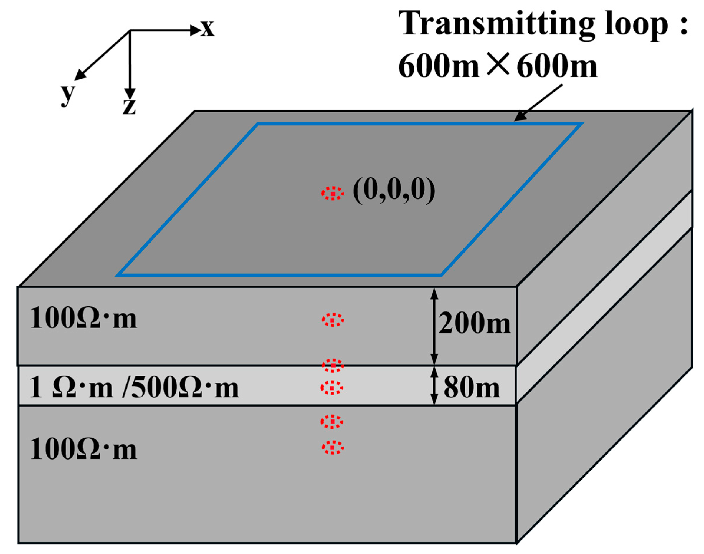
To validate the accuracy of the SEM for both surface and surface-to-tunnel TEM systems, two three-layer earth models have been designed as shown in Figure 2. The thicknesses of the first and second layers are 200 m and 80 m for the two models. The resistivity of the first, second and third layers are 100 Ω·m, 1 Ω·m and 100 Ω·m for one model, while the resistivity of the first, second and third layers are 100 Ω·m, 500 Ω·m, and 100 Ω·m for the other. The key difference between the two layered earth models is that one has a high-resistivity layer as the second layer, while the other has a low-resistivity layer.

The layout of the surface-to-surface and surface-to-tunnel TEM system is as shown in Figure 2. The 1D semi-analytical model is the same as the three-layer earth model in Figure 2. For both the surface and tunnel modes, a surface-based large loop is uniformly adopted as the transmitting source, with receivers deployed on the ground and within the tunnel. The detailed parameters of the TEM system are as follows. The step-off waveform is applied, the transmitting current is 50 A, and the area of the transmitting loop is 600 m × 600 m. The receivers are placed both on the earth surface and within the tunnel. The discrete mesh information we employed for the third and fourth-order SEM verification is as follows. The physical mesh is subdivided into 8800 elements, with a minimum element size of 20 m × 20 m × 40 m. The coordinate origin is set at the midpoint of the transmitting loop, and the receivers are set as (0 m, 0 m, 0 m) on the ground surface and (0 m, 0 m, 120 m), (0 m, 0 m, 200 m), (0 m, 0 m, 240 m), (0 m, 0 m, 300 m), and (0 m, 0 m, 350 m) within the tunnel.

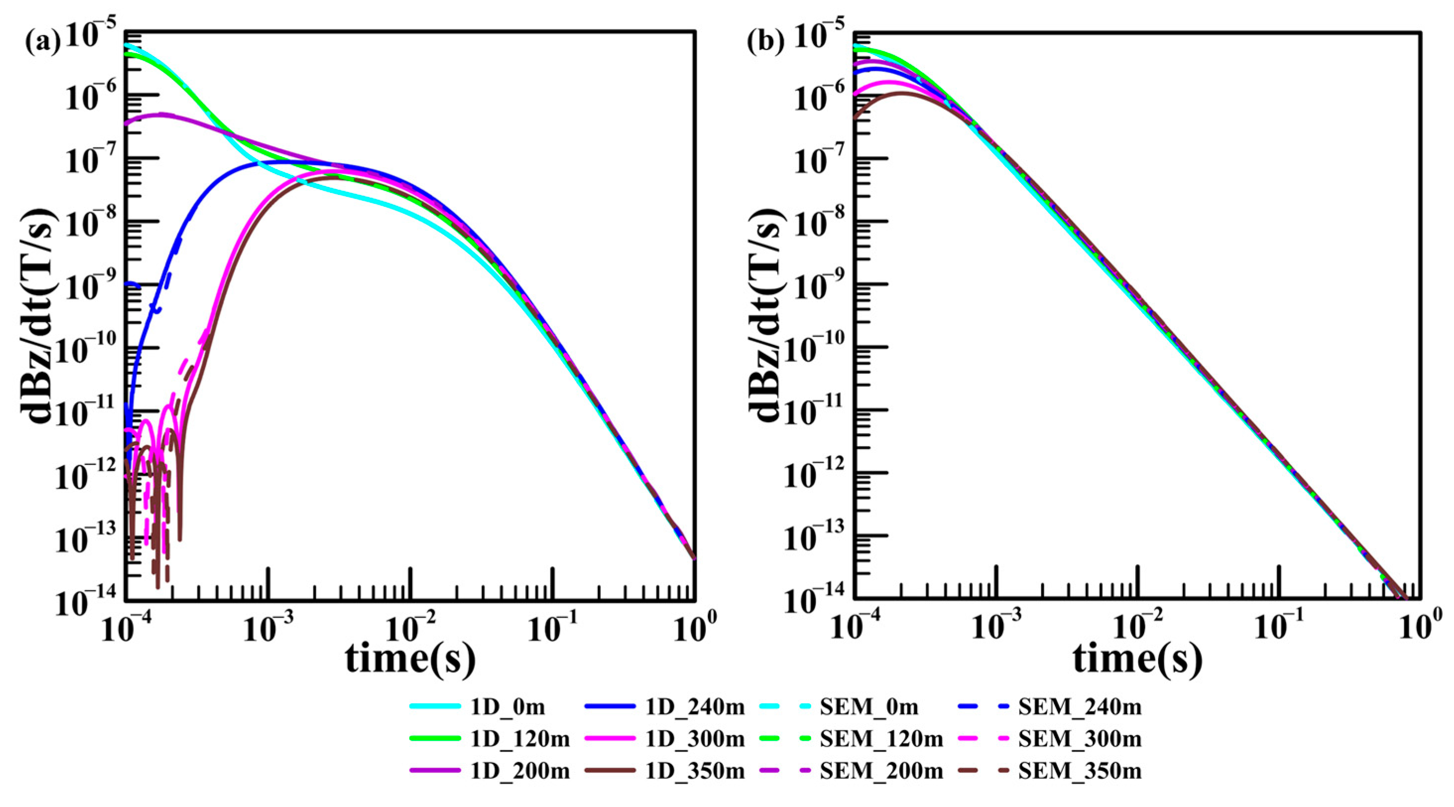
Figure 3a and Figure 3b, respectively, present the dBz/dt response decay curves with time channel of surface and tunnel receivers for the models with a second layer of low resistivity and high resistivity, calculated by the third-order SEM and the 1D semi-analytical solution. From Figure 3, it can be observed that the dBz/dt decay curves for both models calculated by the third-order SEM and the 1D analytical solution are well-fitted with each other, to some extent, which demonstrates the effectiveness of the SEM algorithm. The dBz/dt decay curves of the low-resistivity layer model and the high-resistivity layer model show significant differences. For the low-resistivity layer model, the dBz/dt response characteristics of surface receiver points and those within the low-resistivity layer (tunnel location) differ significantly. The dBz/dt field at the surface receiver point (z = 0 m) and near the surface receiver point (z = 120 m) exhibits a nonlinear attenuation over time. It has an increase in the early time channels and reaches a peak, before decreasing over time, with the receiver located in the low-resistivity layer (z = 200 m, 240 m). As the receiver point (z = 300 m, 350 m) depth increases away from the second low-resistivity layer, the feature of the dBz/dt response curve initially increasing and then decreasing over time weakens (occurring only at very early stages); overall, the dBz/dt field value exhibits a decrease with time. Therefore, the dBz/dt field of the low-resistivity earth model demonstrates that when the receiver point is located within that layer, the dBz/dt field value decays over time with a distinct pattern: it first increases and then decreases during the early-to-middle time period. This dBz/dt response characteristic differs from observations made at the surface, above the low-resistivity layer, or below it, and can be effectively used to identify the low-resistivity target layer. For the high-resistivity layer model, the dBz/dt response curves recorded at the surface (z = 0 m), above the high-resistivity layer (z = 120 m), within it (z = 200 m, 240 m), and below it (z = 300 m, 350 m) all exhibit a similar evolution pattern. During the early time stage, the response value first shows a slight increase and then decays, while in the middle-to-late time stages, it presents a nonlinear decay over time. Additionally, in the early time stages, the observed responses at different receiver points exhibit significant differences, and as the depth z increases, the magnitude of the dBz/dt response decreases accordingly. Compared with a low-resistivity layer model, the dBz/dt response of model with a high-resistivity layer retains a certain degree of identifiability, though this is lower than that of the low-resistivity layer model.

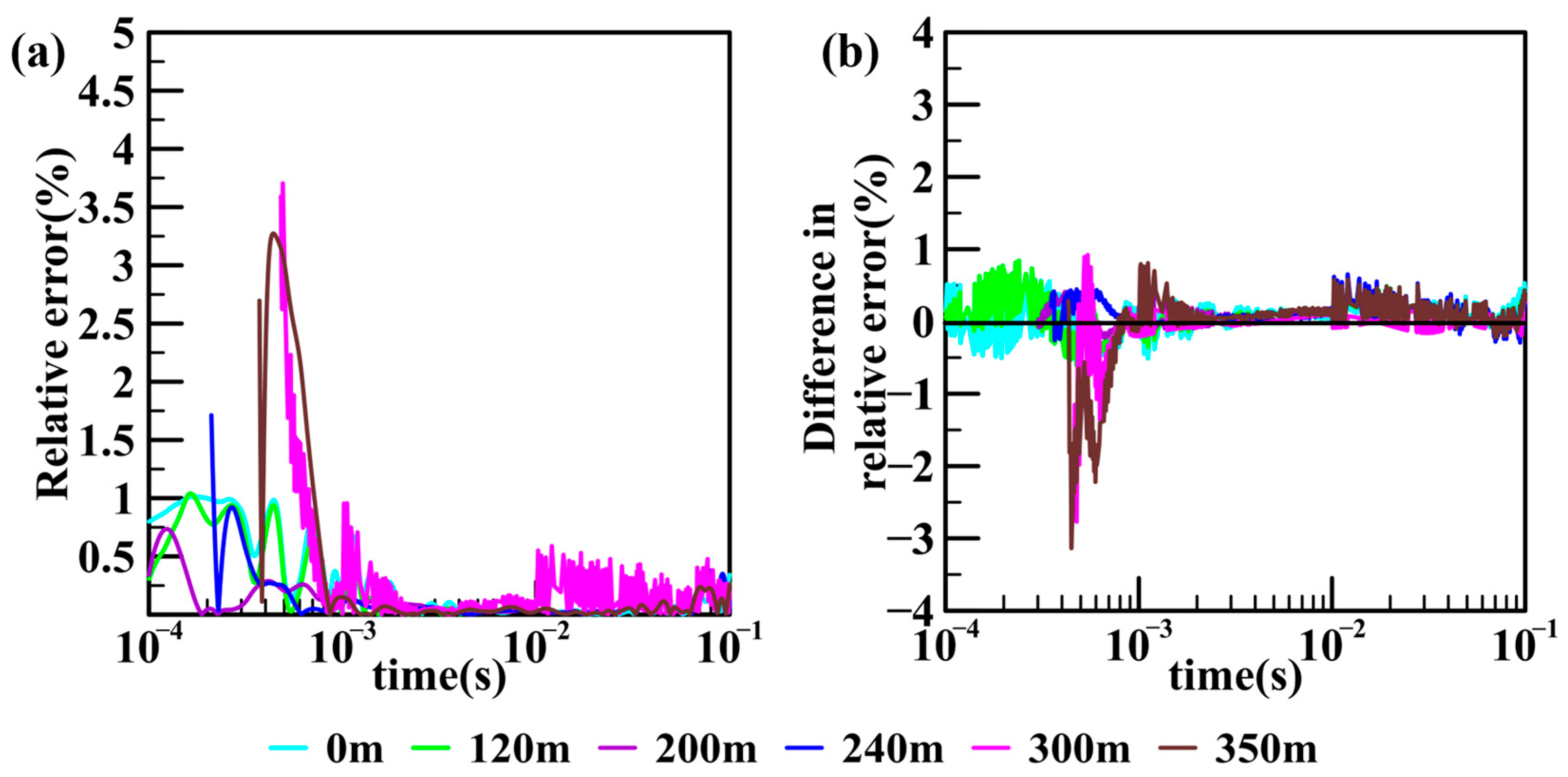
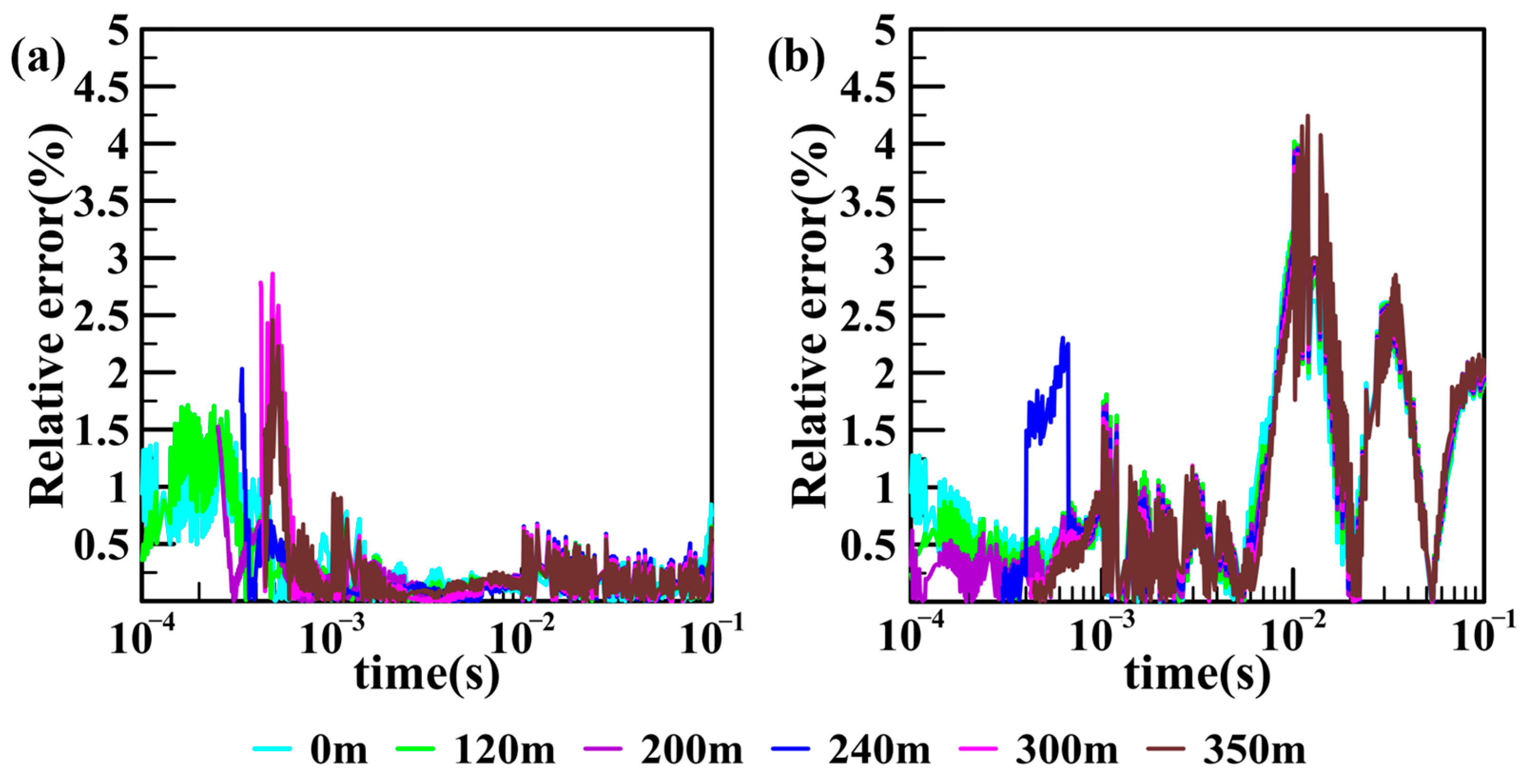
Figure 4 presents the relative errors between the third-order SEM and the 1D semi-analytical solution for both earth models. As shown in Figure 4, the relative errors between the third-order SEM and the semi-analytical solution at multiple surface and tunnel receiver points for both models are less than 5%. This demonstrates the accuracy of the SEM in solving the surface-to-tunnel TEM mode. Furthermore, most of the relative errors remain within 2%. Notably, in Figure 4a, the relative errors are less than 0.5% during the later time interval from 10⁻³ s to 0.1 s, which demonstrates the accuracy of the SEM in solving models containing the low-resistivity layer models. The results further show the application potential of the surface-to-tunnel TEM forward modeling based on SEM in simulating in real models of water-bearing fractured zones in coalfields.

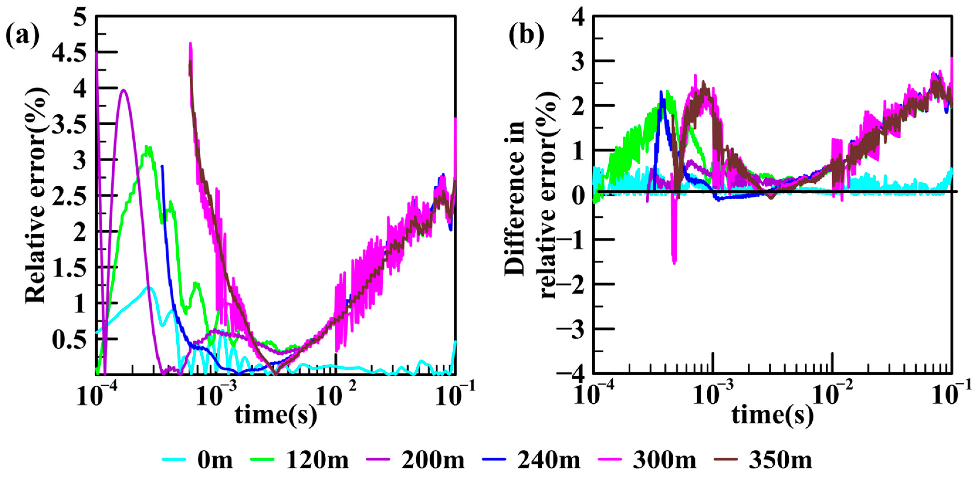
Theoretically, the modeling accuracy of the SEM is influenced by both the order of the basis functions and the physical mesh discretization. For the low-resistivity layer model in Figure 2 (the second layer with resistivity of 1 Ω·m), we individually vary the order of the basis functions and the form of the physical mesh discretization to conduct an in-depth analysis of their impacts on modeling accuracy.

We used the fourth-order SEM to calculate the dBz/dt response for the low-resistivity layer model shown in Figure 2. Figure 5a presents the relative errors between the fourth-order SEM and the 1D semi-analytical solutions; Figure 5b shows the difference in relative errors between the third-order and fourth-order results. As shown in Figure 5a, the relative errors of the fourth-order SEM remain within 5%, with the majority confined below 0.5%. Figure 5b reveals that the relative errors of the third-order SEM results are significantly larger than those of the fourth-order SEM calculations. This observation indicates that the accuracy of surface-to-tunnel TEM forward modeling based on the SEM improves substantially with an increase in the order of the basis functions.

To analyze the impact of mesh discretization on the SEM forward modeling, a coarser element mesh is employed for the low-resistivity layer model shown in Figure 2. The physical mesh was subdivided into 20 × 20 × 20 cells, with a minimum cell size of 30 m × 30 m × 50 m, and third-order basis functions are similarly used for the modeling. The relative errors between the results from the coarse mesh SEM and the 1D semi-analytical solution are shown in Figure 6a, while the differences in relative errors between the coarse and fine mesh results are presented in Figure 6b. Figure 6 indicates that the SEM results from the coarse mesh exhibit good agreement with the semi-analytical solution, with most relative errors remaining within 2%. However, as the receiver point moves deeper below the surface, the errors increase, particularly evident in the early time channels. In summary, although the coarse mesh we employed essentially maintains the required accuracy, the relative errors of the coarse mesh SEM results are generally larger than those obtained from the fine mesh.

Therefore, for 3D surface and surface-to-tunnel TEM forward modeling based on the SEM, both increasing the order of basis functions and optimizing mesh discretization can improve modeling accuracy.

4. Detection Capability Analysis of Surface and Surface-to-Tunnel TEM Response Characteristics for Typical Models

4.1. 3D Earth Model Design

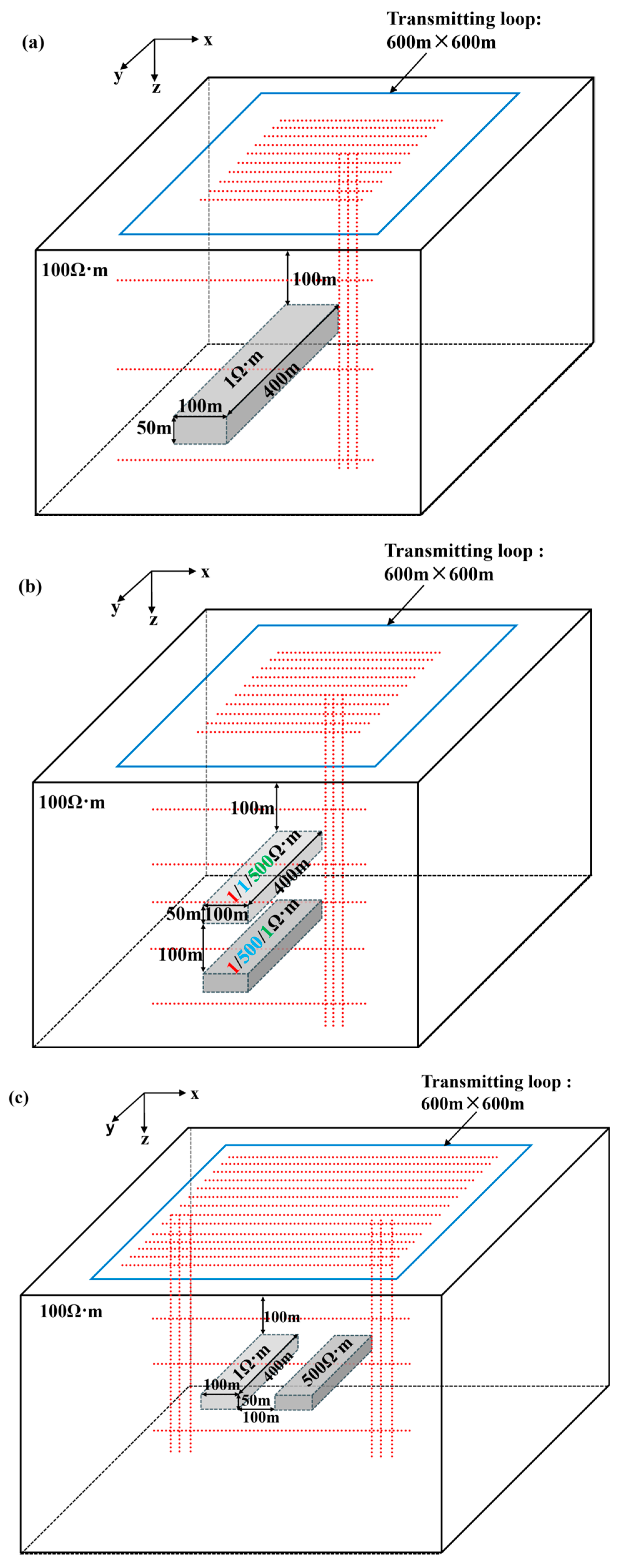
For the TEM dBz/dt response calculation of the 3D model, we employed the same TEM system as shown in Figure 2. To analyze the detection capabilities of the surface-to-surface TEM and surface-to-tunnel TEM under different geological background conditions, three earth models are designed for coalfield conditions, as shown in Figure 7; one is a single anomalous body model (Model A), one is dual anomalous bodies with one deep and one shallow burial depth (Model B), and one is dual anomalous bodies with the same burial depth (Model C). The size of all burial anomalous bodies is consistent at 100 m × 400 m × 50 m, and the background resistivity is 100 Ω·m. The burial top surface of the anomalous bodies for Models A and C is at a depth of 100 m. In Model B, the vertical distance between the upper and lower anomalous bodies is 100 m (one burial depth is 100 m, the other is 200 m), while in Model C, the horizontal distance between the left and right anomalous bodies is 100 m. The resistivity information of the anomalous bodies is as shown in

Table 1. Parameters for anomalous earth models shown in Figure 7.

	Types and Abbreviations	Resistivity	Center Position of the Anomalous Bodies
Model A	Single low-resistivity anomalous body (L Model)	1 Ω·m	(0 m, 0 m, 125 m)
Model B	Dual low-resistivity anomalous bodies (LL Model)	Both 1 Ω·m	(0 m, 0 m, 125 m) and (0 m, 0 m, 275 m)
	Upper low-resistivity and lower high-resistivity dual anomalous bodies (ULLH Model)	1 Ω·m and 500 Ω·m	(0 m, 0 m, 125 m) and (0 m, 0 m, 275 m)
	Upper high-resistivity and lower low-resistivity dual anomalous bodies (UHLL Model)	500 Ω·m and 1 Ω·m	0 m, 0 m, 125 m) and (0 m, 0 m, 275 m)
Model C	Left low-resistivity and right high-resistivity dual anomalous bodies (LLRH Model)	1 Ω·m and 500 Ω·m	(100 m, 0 m, 125 m) and (−100 m, 0 m, 275 m)

. For the dual anomalous bodies in Model B, we set three kinds of resistivity parameters as follows: (1) both anomalies are low-resistivity bodies (1 Ω·m); (2) the shallow-buried anomaly is a low-resistivity body (1 Ω·m), while the deep-buried anomaly is a high-resistivity body (500 Ω·m); and (3) the shallow-buried anomaly is a high-resistivity body (500 Ω·m), while the deep-buried anomaly is a low-resistivity body (1 Ω·m). For the dual anomalous bodies in Model C, we set both anomalies as low-resistivity bodies (1 Ω·m).

To assess the above five kinds of earth models, we conducted TEM forward modeling for both the large-area surface-to-surface TEM mode and the single-line surface-to-tunnel TEM mode. This integrated approach, combining surface-area scanning with a surface-to-tunnel survey line, effectively fits the operational realities of actual exploration. Due to the spatial constraint of the working environment, receiver points in the tunnel are generally limited to the deployment of a single survey line along its axis, employing either a horizontal or vertical electrode array. By deploying multiple survey lines, earth surface areas achieve a spatially dense, area-wide receiver points layout. For Models A, B and C, the receiver points layouts for the surface-to-surface TEM are the same; the survey area is defined as a 400 m × 400 m grid centered at (0 m, 0 m, 0 m), with a receiver point spacing of 10 m.

Regarding the tunnel receiver points layout, it contains horizontal and vertical survey lines. (1) Vertical survey line: Models A and B share the same survey line deployment. Vertical survey lines are deployed on the right side of the anomalous body at x = 50 m, 60 m, and 70 m. Each survey line starts at the surface at (50 m, 0 m, 0 m), (60 m, 0 m, 0 m), and (70 m, 0 m, 0 m), respectively, and extends to 400 m depth with 10m spacing along the z-axis. Model C uses a similar survey line deployment to Models A and B, but is positioned differently. Model C’s vertical survey lines are deployed on the right side of the right anomalous body at x = 150 m, 160 m, and 170 m, and on the left side of the left anomalous body at x = −150 m, −160 m, and −170 m. Each survey line starts at the surface at (150 m, 0 m, 0 m), (160 m, 0 m, 0 m), (170 m, 0 m, 0 m), (−150 m, 0 m, 0 m), (−160 m, 0 m, 0 m), and (−170 m, 0 m, 0 m), respectively, and extends to 400 m depth with 10m spacing along the z-axis. (2) Horizontal survey line: Models A and C share the same survey line deployment. The survey lines are distributed horizontally at three depths: above the anomalous body (z = 50 m), within it (z = 125 m), and below it (z = 200 m). The survey lines extend from (−200 m, 0 m) to (200 m, 0 m) with 10m spacing along the x-axis. Model B uses the same survey lines deployment as Models A and C, plus two additional survey lines: within the lower anomalous body (z = 275 m) and below it (z = 350 m).

4.2. Response Characteristics and Analysis of Surface-to-Surface TEM Mode

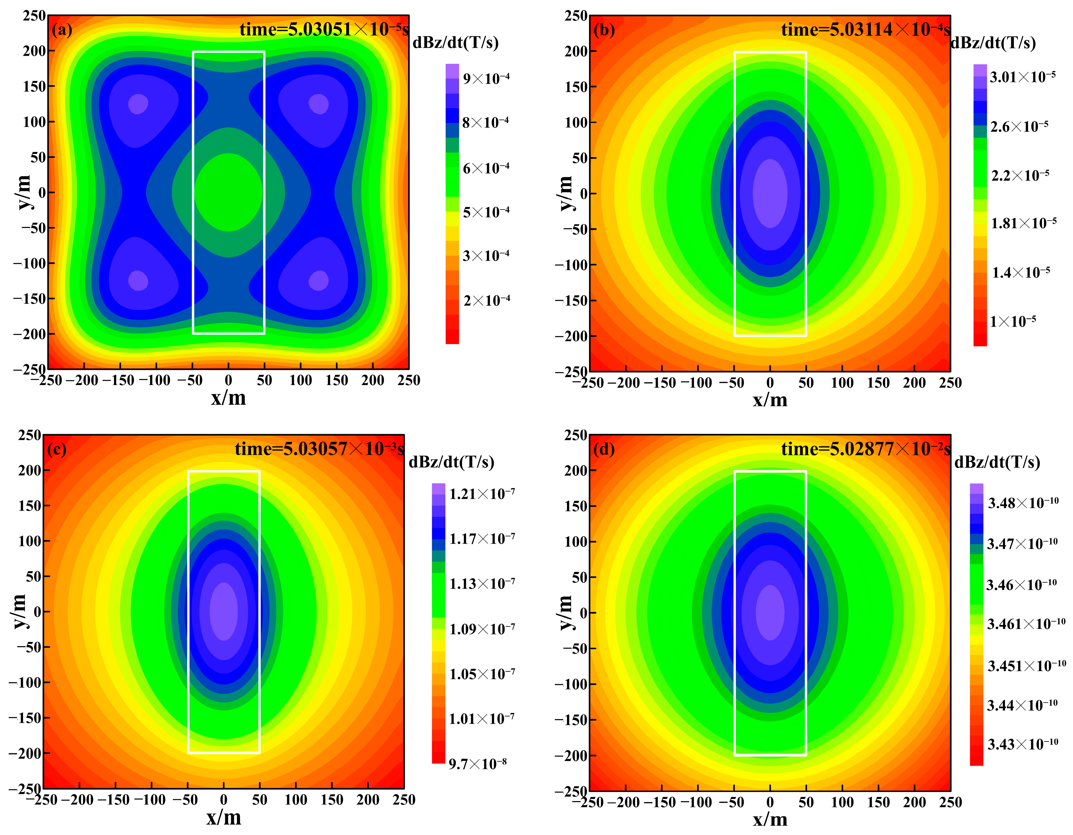
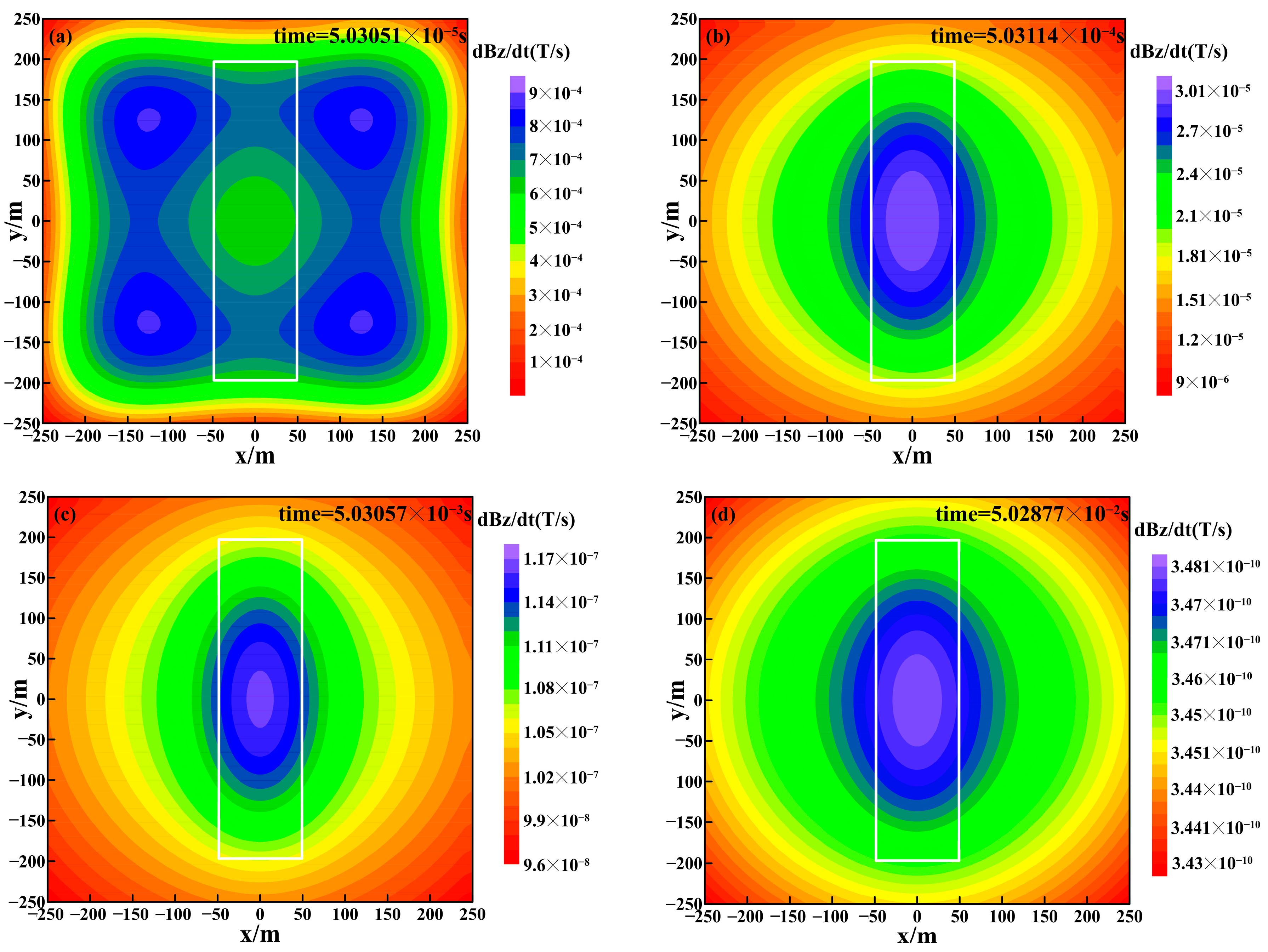
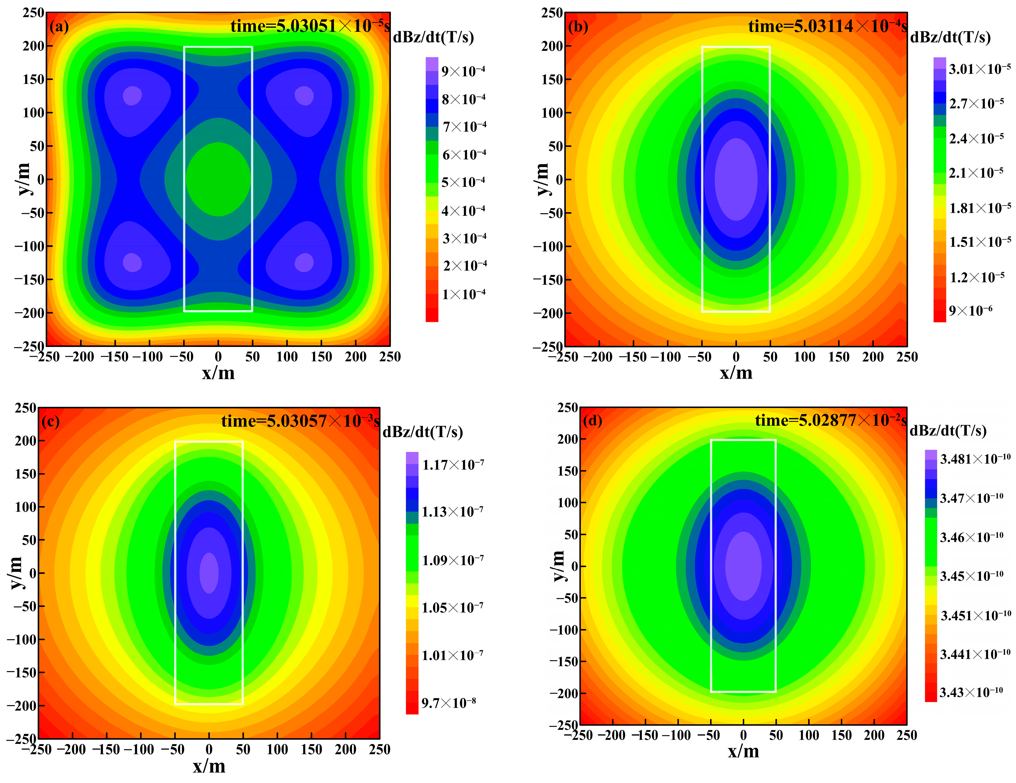
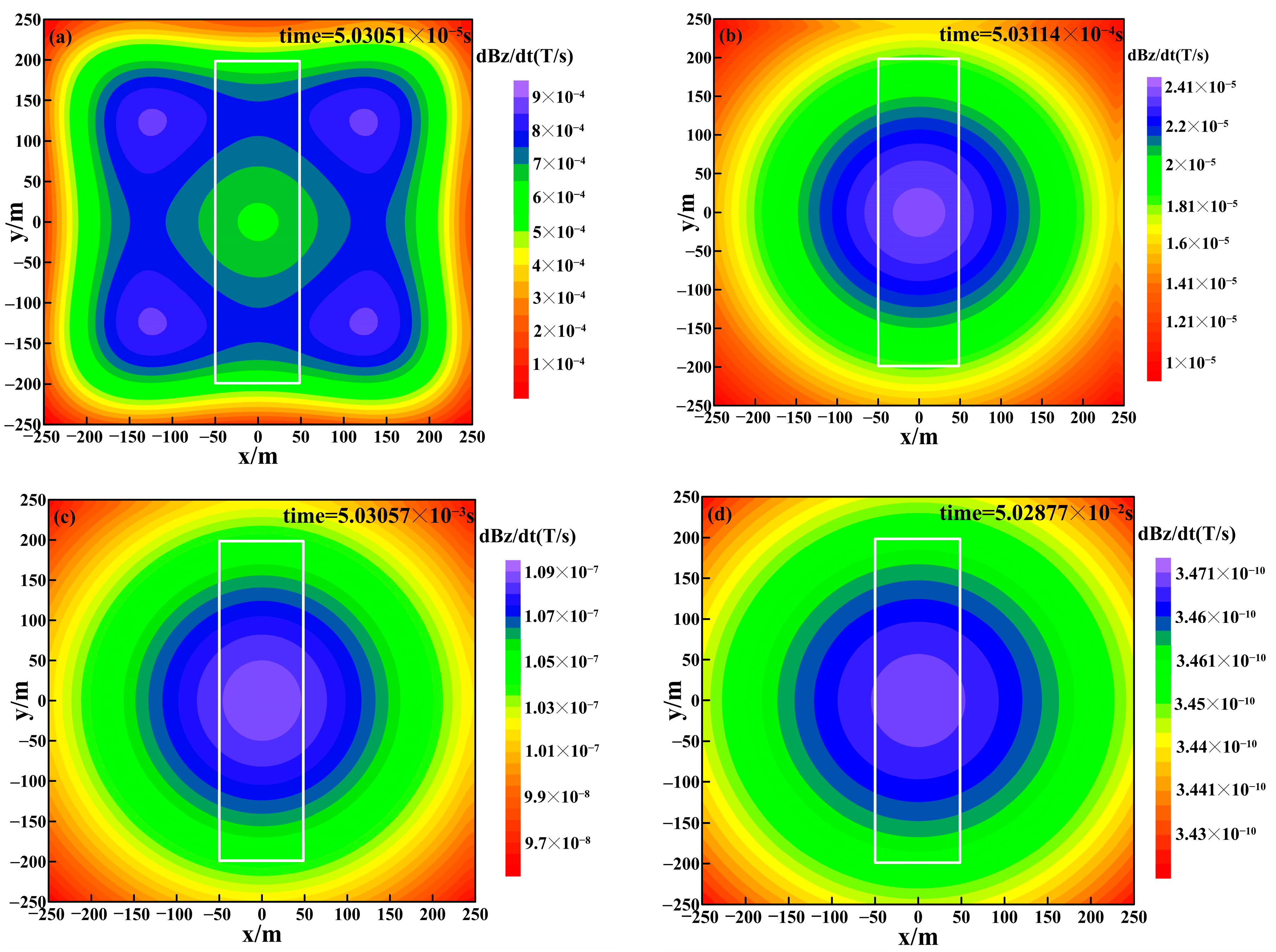
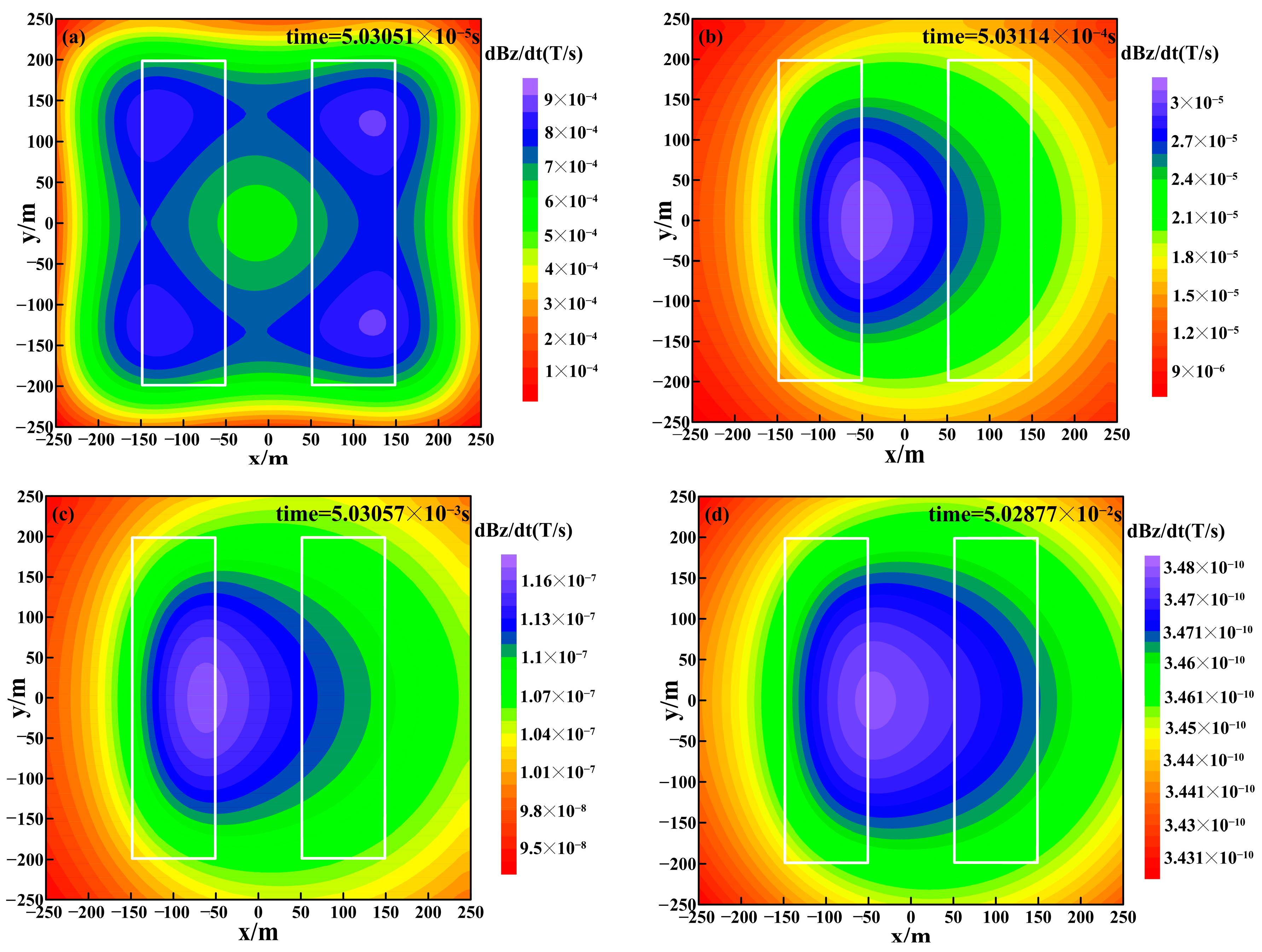
Figure 8, Figure 9, Figure 10, Figure 11 and Figure 12 are the multi-survey line contour plots of the multiple time channels (time = 5.03051 × 10⁻⁵ s, 5.03114 × 10⁻⁴ s, 5.03057 × 10⁻³ s, 5.02877 × 10⁻² s) surface-to-surface dBz/dt response for the above five 3D earth models (L, LL, ULLH, UHLL and LLRH models). Figure 8 shows the dBz/dt response distributions for the L model at different time channels. The dBz/dt response patterns are axisymmetric about the single anomalous body at different time channels. Based on the distribution characteristics of dBz/dt responses in the x–y plane, we can see that the strongest response occurs for x = −50 m to 50 m and y = −200 m to 200 m, which indicates that the anomalous body extends roughly over these ranges.

In Figure 9, Figure 10 and Figure 11, the surface response is essentially identical to that shown in Figure 8, while the dBz/dt response magnitude exhibits some variations. This indicates that the anomalous bodies extend roughly from x = −50 m to 50 m and y = −200 m to 200 m. When the horizontal positions of two anomalous bodies coincide and only their burial depths differ, the dBz/dt response characteristics observed at the surface receiver locations resemble those of a single anomalous body, making it difficult to distinguish between the two. For the UHLL Model, the characteristics of the dBz/dt contour response in the x-y plane differ somewhat from those of the L and LL models. This is likely due to the presence of a shallow high-resistivity body, causing the planar response to approximate a circular shape, which diminishes the ability to identify boundaries in both the x- and y- directions.

Figure 12 shows the surface dBz/dt response distributions for the LLRH model at different time channels. Figure 12 shows that the surface dBz/dt response has a certain ability to identify horizontal dual anomalous bodies, with a greater ability to identify low-resistivity anomalous bodies. The surface dBz/dt response contour characteristics of the LLRT model differ significantly from those of the three previously discussed models. This dissimilarity arises from the presence of two laterally adjacent anomalous bodies with distinct resistivity values within the model, with the low-resistivity anomaly on the left side exerting a more dominant influence on the surface response. As illustrated in Figure 12, the zone of peak response exhibits a leftward shift, while the right-side response remains comparatively subdued. This pattern indicates that the left anomaly extends approximately within the region defined by x = −50 m to 50 m and y = −200 m to 200 m, while the right anomaly occupies the spatial domain from x = 50 m to 150 m along the y = −200 m to 200 m interval.

Based on the surface-to-surface dBz/dt response characteristics of the above five 3D earth models, we can draw the following conclusions: (1) For the LL, ULLH and UHLL models, despite vertical differences in the number and resistivity of anomalous bodies, the upper bodies are all low-resistivity, yielding similar surface response characteristics. (2) Although the UHLL model has the same dual-body configuration as the LL and ULLH models, its high-resistivity upper body leads to differences from the LL and ULLH models. (3) The LLRH model consists of two horizontally adjacent anomalous bodies with different resistivities. The left low-resistivity body exerts a significantly stronger influence, shifting the maximum-response region leftward, while the right-side response remains relatively weak. Overall, surface-to-surface TEM has a relatively good ability to identify horizontal boundaries, especially for low-resistivity targets. For targets with overlapping horizontal positions, vertical-direction observations are needed to aid in their identification.

4.3. Response Characteristics and Analysis of Surface-to-Tunnel TEM Mode

4.3.1. Response Characteristics and Analysis of the Tunnel x-Axis Direction Observation

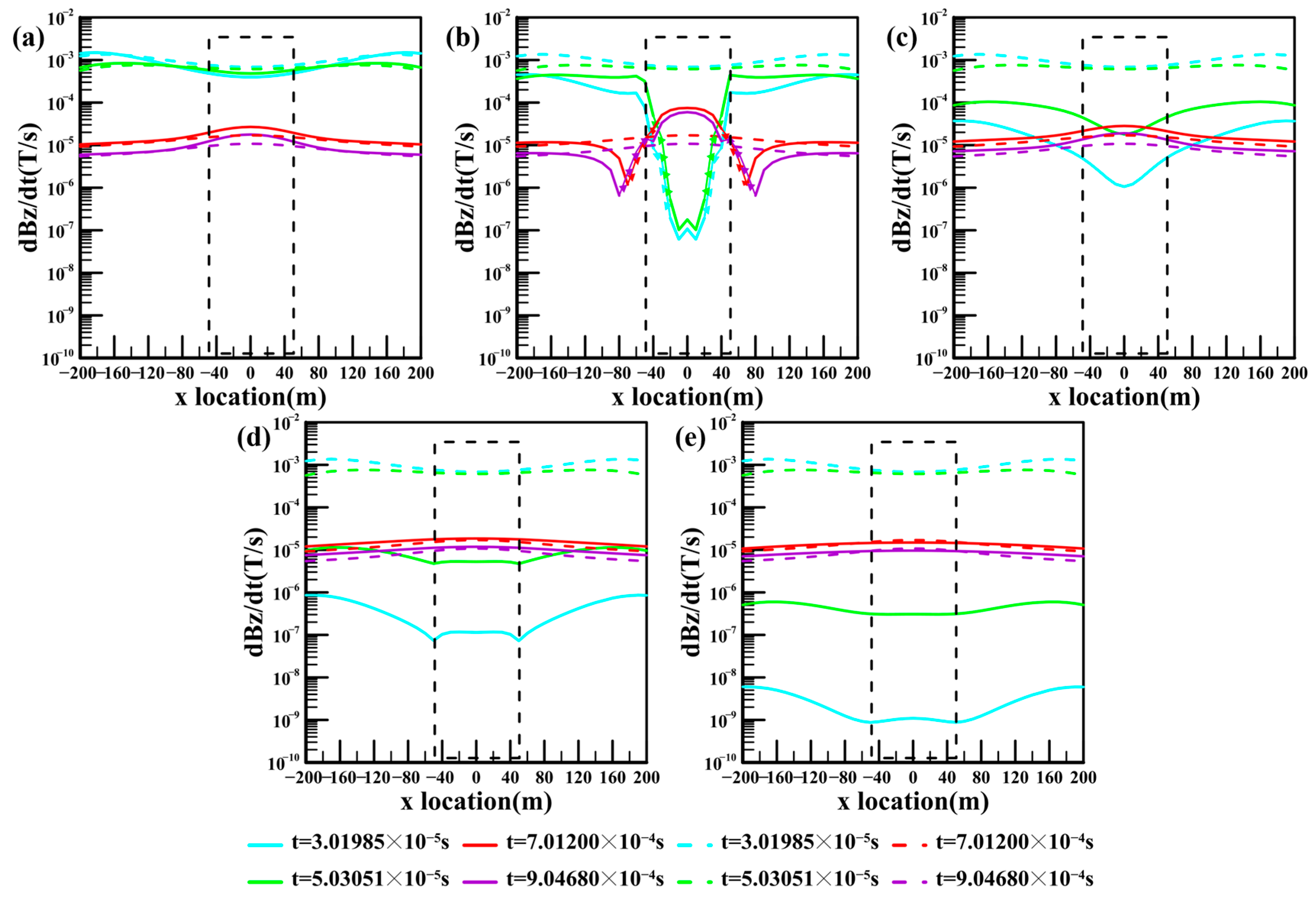
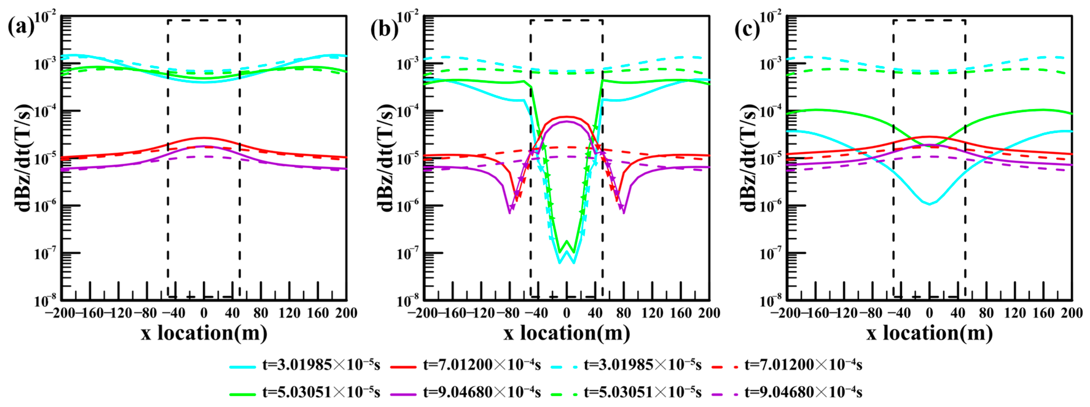
Figure 13 presents the surface-to-surface and surface-to-tunnel dBz/dt response along the x-axis direction survey line for the L model at different time channels. Figure 13 shows that the surface-to-surface dBz/dt responses exhibit smaller amplitude variations near the anomalous body compared to surface-to-tunnel dBz/dt results. This indicates that during TEM exploration, the tunnel survey lines closer to the geological target exhibit enhanced identification capabilities.

The early dBz/dt response is strong and attenuates gradually with time. With increasing depth, the dBz/dt response amplitude progressively decreases. A distinct peak appears near the anomalous body: before 10⁻⁵ s the response curve bulges downward, whereas after 10⁻⁵ s it bulges upward. Notably, in Figure 13b, pronounced fluctuations are observed in the anomalous body around z = 125 m, and the dBz/dt response undergoes a clear reversal between t = 10⁻⁵ s and 10⁻⁴ s. This indicates that the anomalous body is distributed approximately within the horizontal range x = −50 m to 50 m, with a concentration near z = 125 m in the vertical (z-axis) direction.

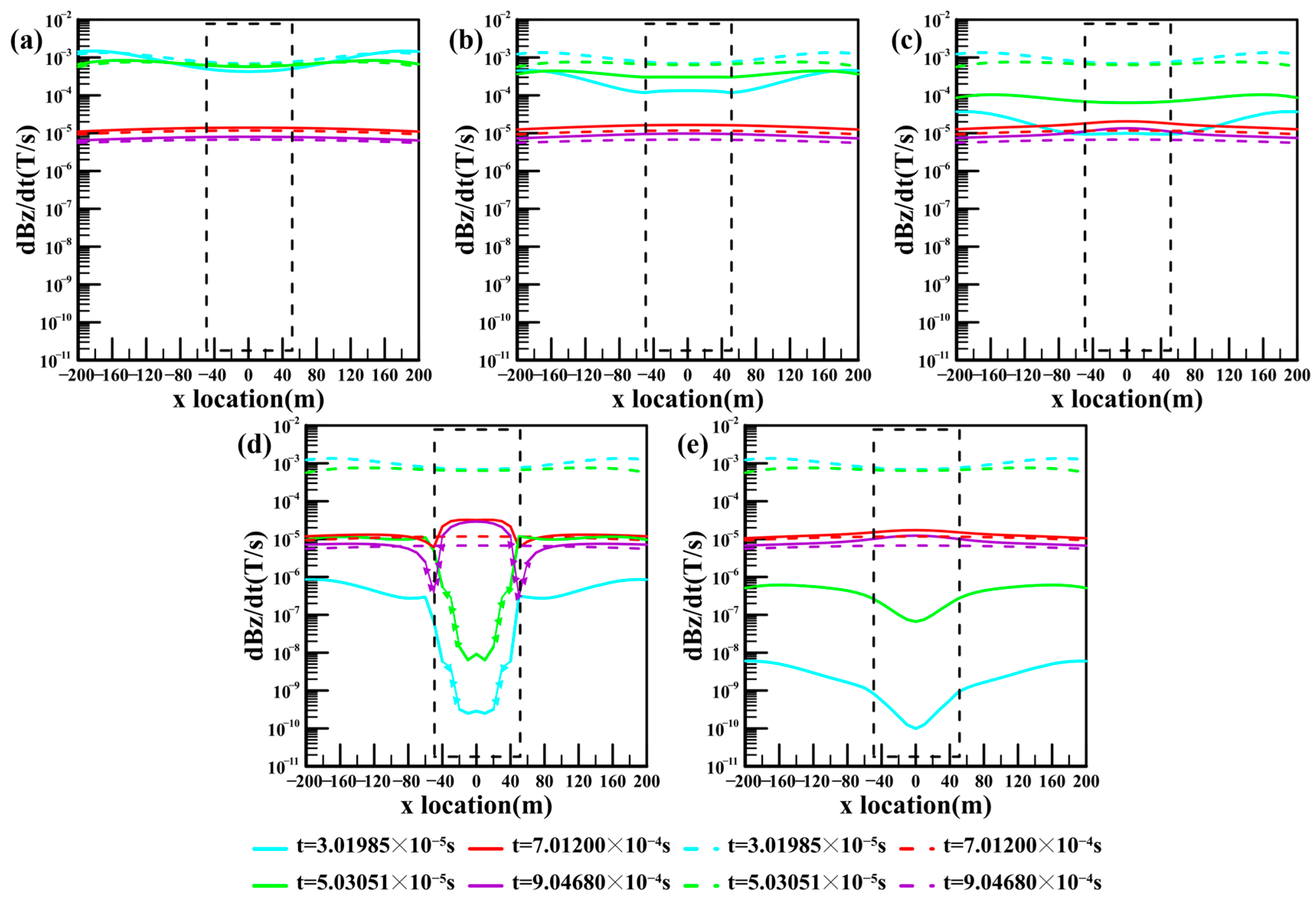
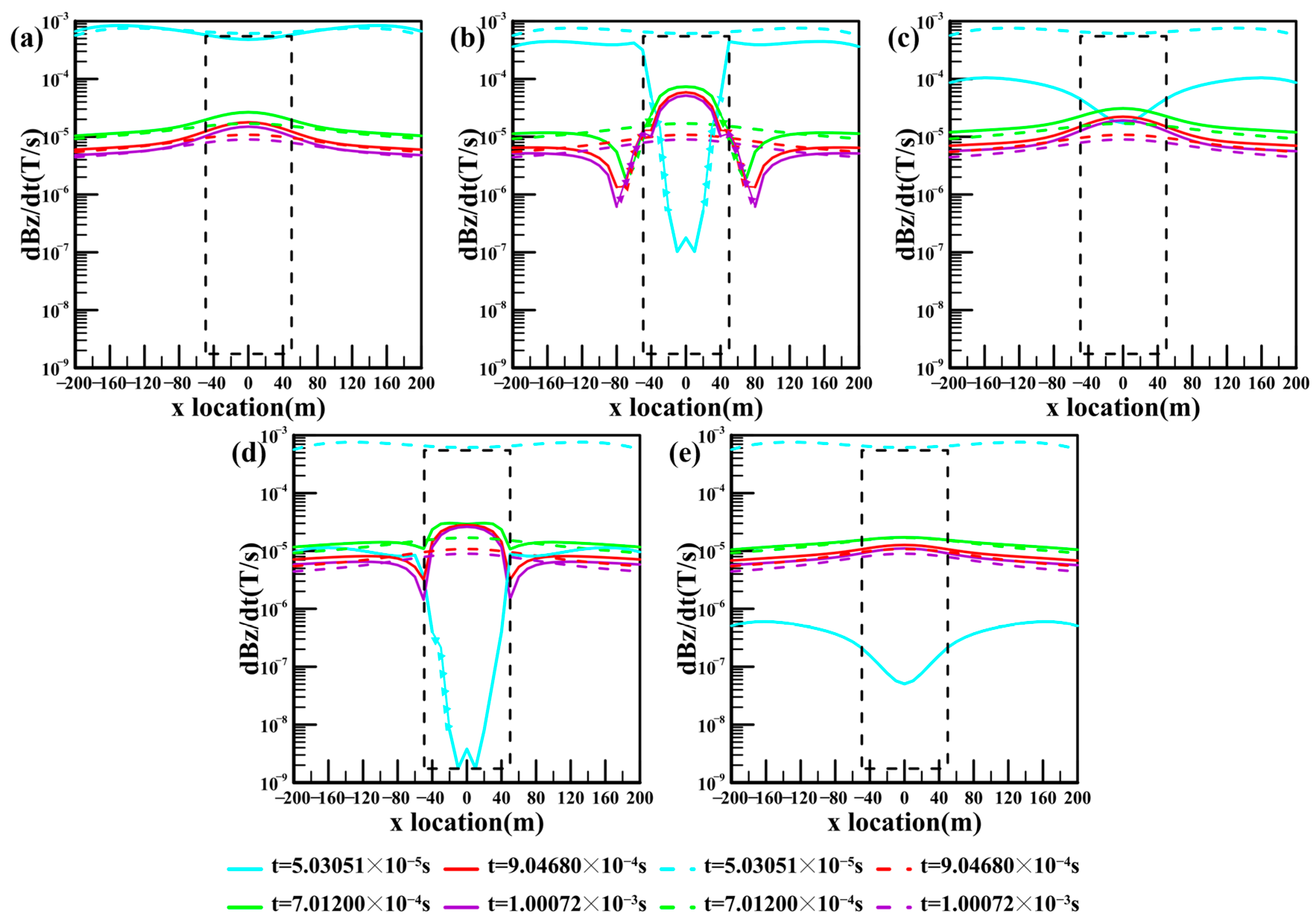
Figure 14 shows the surface-to-surface and surface-to-tunnel dBz/dt response along the x-axis direction survey line for the LL model at different time channels. Similarly, it can be observed that the amplitude variation in tunnel observations near the anomalous body is greater than that of surface survey line observations, indicating that tunnel survey lines closer to the geological target exhibit enhanced identification capability. The dBz/dt responses in Figure 14a–c are essentially the same as those in Figure 13, while the dBz/dt response magnitude exhibits some variations. The dBz/dt responses shown in Figure 14b,d are essentially identical, except that Figure 14d exhibits a slightly weaker dBz/dt response in the early time channels. Figure 14b displays the internal response of the overlying low-resistivity anomalous body, whereas Figure 14d illustrates the response of the underlying high-resistivity anomalous body; this difference likely accounts for the observed variation. The overlying low-resistivity anomalous body attenuates the electromagnetic signal, leading to a weaker early time response in Figure 14d. Similarly, the dBz/dt responses in Figure 14c and Figure 14e are largely consistent, with the only distinction being a moderately attenuated dBz/dt response in the early time channels of Figure 14e. Figure 14c corresponds to the electromagnetic response beneath the overlying low-resistivity anomaly, while Figure 14e reflects the response of the underlying high-resistivity anomalous body, which provides a plausible explanation for the discrepancy. Both overlying anomalous bodies contribute to signal attenuation, resulting in the reduced early time response intensity observed in Figure 14e. As depth increases, the response amplitude demonstrates a gradual decreasing trend.

In Figure 14b,d, prominent fluctuations are evident within the anomalous bodies near z = 125 m and z = 275 m. Notably, within the upper low-resistivity anomalous body, the dBz/dt response undergoes a clear sign reversal between t = 10⁻⁵ s and 10⁻³ s. This indicates that the two anomalous bodies are distributed approximately within the horizontal range of x = −50 m to 50 m, with the upper anomaly centered at z = 125 m and the lower one centered at z = 275 m.

Figure 15 shows the surface-to-surface and surface-to-tunnel dBz/dt response along the x-axis direction survey line for the ULLH model at different time channels. Likewise, it can be observed that when a high-resistivity anomalous body is present, the amplitude variation in the dBz/dt response from tunnel surveys near the anomalous body remains greater than that obtained from surface survey lines, with the tunnel survey lines closer to the geological target still demonstrating superior detection capability. The dBz/dt response characteristics in Figure 15a–c are essentially consistent with those in Figure 14a–c. However, there is a significant difference between the responses in Figure 15d,e and Figure 14d,e, specifically manifested as a marked reduction in amplitude fluctuations. This attenuation in response magnitude likely stems from fundamental differences in the electrical structure between the two types of models: the ULLH model assumes the lower anomalous body to be a high-resistivity body, whereas the LL model assumes it to be a low-resistivity body. These two distinct electrical anomalous bodies exert differential influences on the diffusion and attenuation processes of the electromagnetic field. Notably, in Figure 15b, substantial dBz/dt response fluctuations can still be observed within the anomalous body near z = 125 m. Particularly prominent is the clear sign reversal of the dBz/dt response in the upper low-resistivity anomalous body during the time interval from t = 10⁻⁵ s to 10⁻³ s. These response characteristics indicate that the two electrical anomalous bodies extend approximately horizontally between x = −50 m and 50 m, with the center of the upper anomalous body lying at about 125 m depth and that of the lower one at about 275 m depth. Based on the above information, the horizontal boundaries of the target bodies can be effectively delineated.

Figure 16 shows the surface-to-surface and surface-to-tunnel dBz/dt response along the x-axis direction survey line for the UHLL model at different time channels. For the UHLL model, significant amplitude variation is observed near the lower low-resistivity anomalous body (as shown in Figure 16b), while the response amplitude near the upper high-resistivity anomalous body remains relatively weak (Figure 16d). Notably, within the lower low-resistivity anomalous body, the dBz/dt response exhibits a distinct sign reversal in the time range of t = 10⁻⁵ to 10⁻³ s. This indicates that both anomalous bodies extend approximately horizontally from x = −50 m to 50 m, with the upper body centered at a depth of z = 125 m and the lower body at z = 275 m.

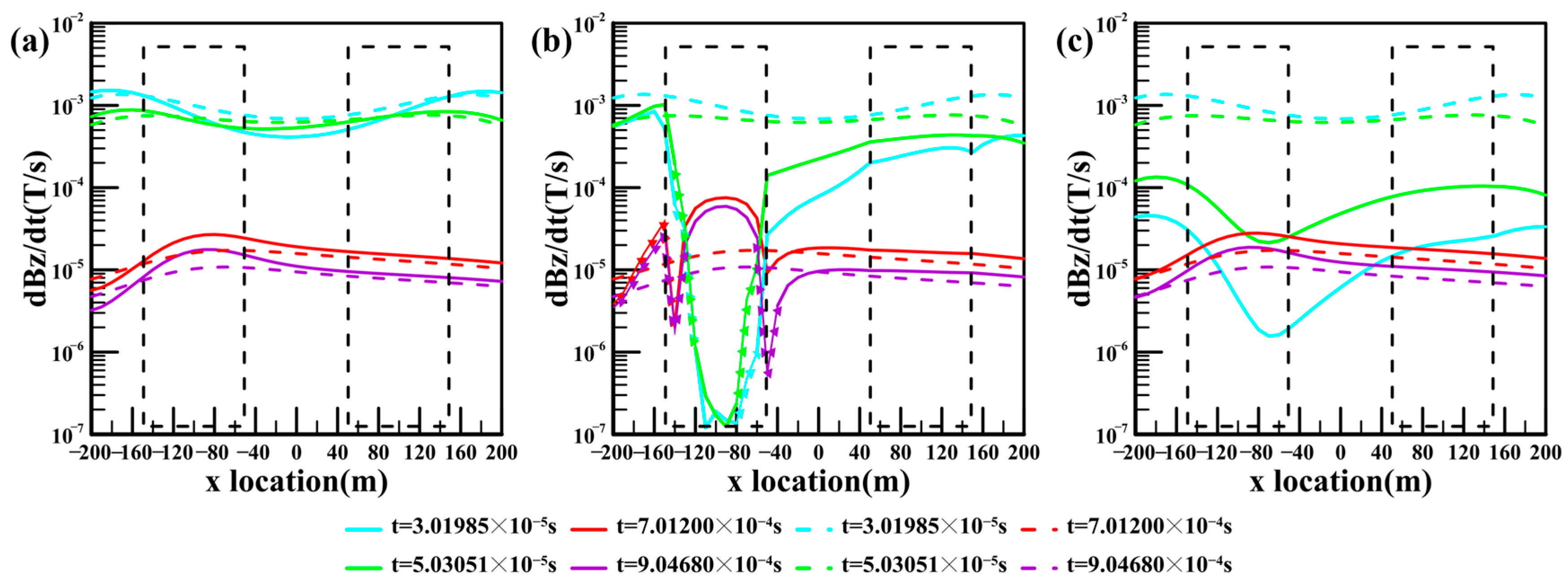
Figure 17 shows the surface-to-surface and surface-to-tunnel dBz/dt responses along the x-axis direction survey line for the LLRH model at different time channels. For a model containing both a low-resistivity and a high-resistivity anomaly at the same burial depth, the dBz/dt response amplitude variation obtained through tunnel-based observations near the anomalies is still larger than that from surface survey lines, indicating that the tunnel survey line closer to the geological target retains better recognition capability.

The LLRH model consists of two laterally adjacent geological bodies with distinct electrical resistivities. The low-resistivity anomalous body on the left dominates the distribution characteristics of the dBz/dt response, while the dBz/dt response amplitude variations near the high-resistivity anomalous body on the right are comparatively weaker. As illustrated in Figure 17b, more pronounced fluctuations in the dBz/dt response amplitude can be observed, with significant dBz/dt response amplitude variations localized primarily within the anomalous bodies near the depth of z = 125 m. Notably, within the left low-resistivity anomalous body, the dBz/dt response exhibits a distinct sign reversal over the time interval from t = 10⁻⁵ s to 10⁻³ s. The response curves indicate that both anomalous bodies are centered at a depth of z = 125 m; the left body roughly extends laterally between x = −150 m and −50 m, while the right body spans from x = 50 m to 150 m.

Based on the surface-to-tunnel dBz/dt response characteristics of the above five 3D earth models, we can draw the following conclusions: (1) For all 3D earth models with varying anomalous body configurations, the dBz/dt response curves consistently show that the amplitude variation near the anomalies is larger in tunnel-based surveys than in surface-based surveys. This demonstrates that survey lines positioned closer to geological targets in tunnels possess superior capabilities for anomaly detection. To some extent, this further indicates that integrated surface and tunnel-based TEM observation contributes to high-resolution detection of the target bodies, specifically for the detection and identification of the burial low-resistivity anomalous bodies. (2) The LL and ULLH models both feature a dual upper–lower anomalous body configuration. Their dBz/dt responses differ because the lower anomalous body is low-resistivity in the LL model and high-resistivity in the ULLH model. (3) The ULLH and UHLL models differ because their upper and lower anomalous bodies are interchanged, leading to significant fluctuations. (4) The LLRH model comprises two adjacent anomalous bodies of different resistivity, with the left low-resistivity body producing more pronounced horizontal response fluctuations.

4.3.2. Response Characteristics and Analysis of the Tunnel z-Axis Direction Observation

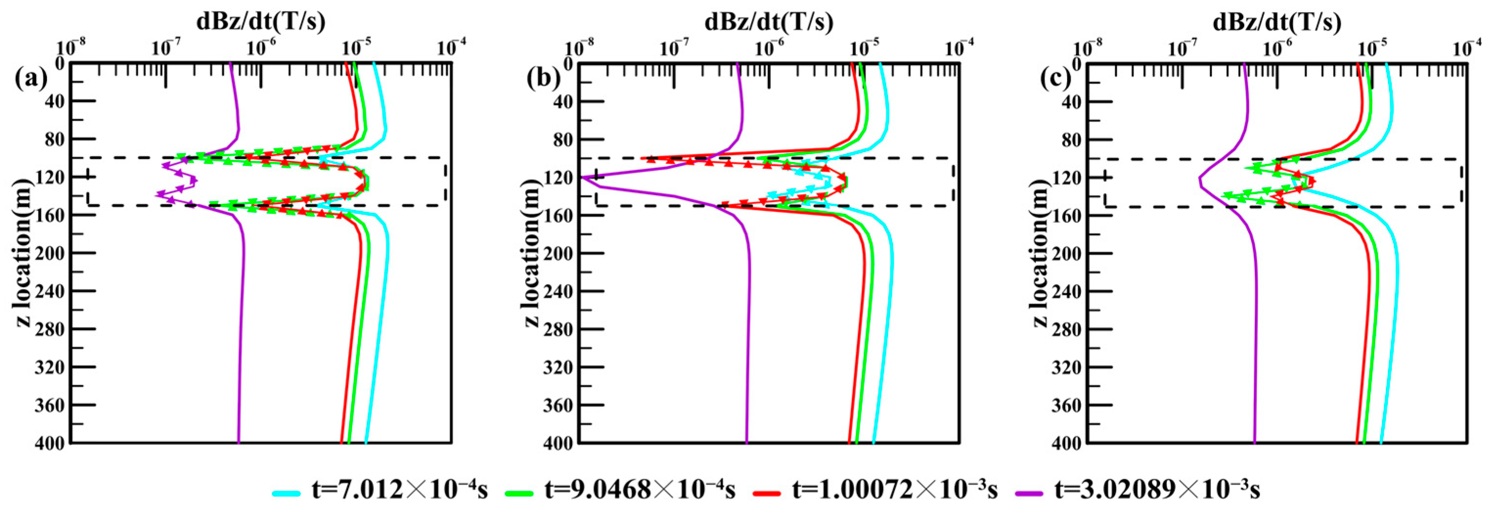
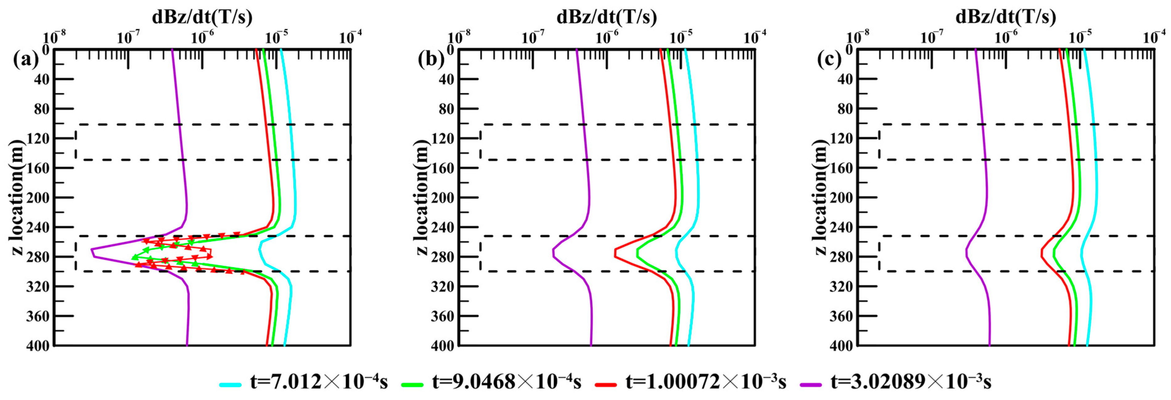
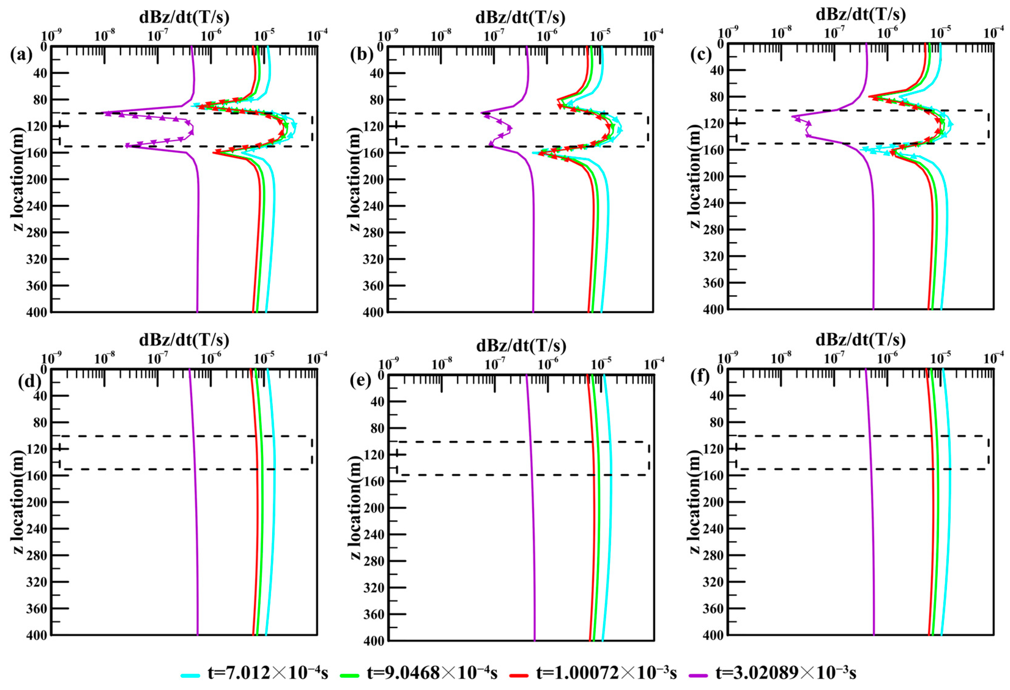
Figure 18 shows the surface-to-tunnel dBz/dt response along the z-axis direction survey line for the L model at different time channels. The observation dBz/dt results along the z-direction in the tunnel show a significant variation in dBz/dt response amplitude at the top and bottom interfaces of the anomalous body, enabling clear identification of the upper and lower boundaries of the low-resistivity target. During the early time channels, the amplitude of the dBz/dt response is strong and attenuates gradually over time. Prominent fluctuations in dBz/dt response amplitude occur near the anomalous body, accompanied by a distinct sign reversal of the dBz/dt response between t = 10⁻⁴ s and 10⁻³ s. The location of these dBz/dt response variations coincides with the burial depth of the anomalous body, which lies between z = 100 m and 150 m. Furthermore, as the dBz/dt observation line moves away from the target body, the variations in the dBz/dt response weaken to a certain extent, and the sign-reversal phenomenon gradually diminishes with increasing distance. Thus, it can clearly be observed that dBz/dt observations along the z-direction in the tunnel contribute effectively to identifying the vertical boundaries of the low-resistivity target body.

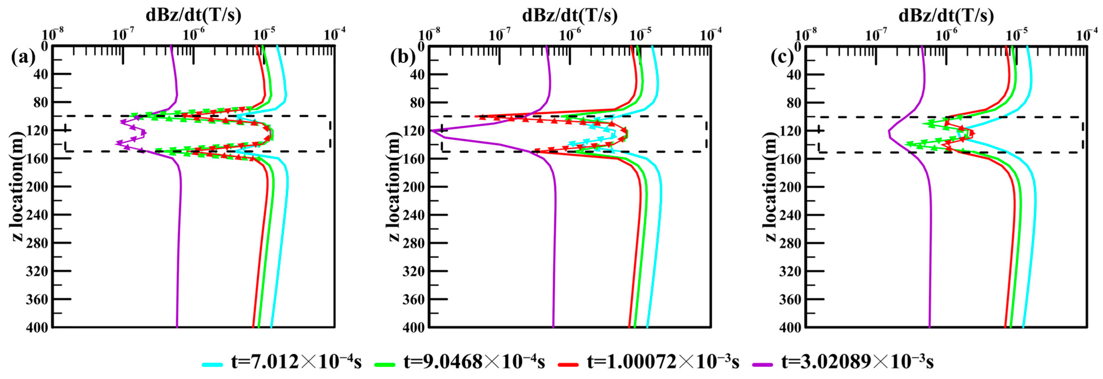
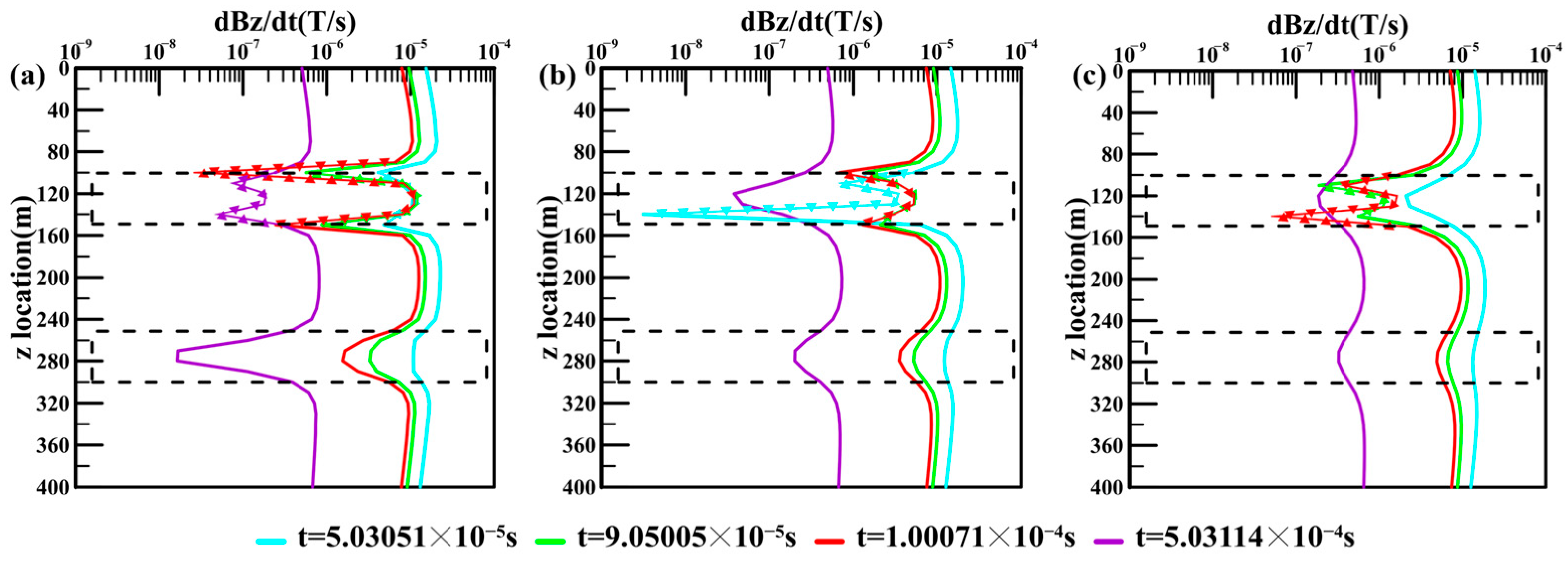
Figure 19 shows the surface-to-tunnel dBz/dt response along the z-axis direction survey line for the LL model at different time channels. The LL model contains two low-resistivity anomalous bodies with identical horizontal dimensions but different burial depths. Based on the results from the previous surface-based observations and horizontal tunnel surveys, it has been established that effectively separating and identifying the two anomalous bodies presents significant difficulty. From Figure 19, we can find that the distribution of the dBz/dt responses along z-direction tunnel survey line reveals two distinct amplitude variations in the dBz/dt response curves for multiple time channels. The locations of the dBz/dt response amplitude changes show excellent correspondence with the positions of the top and bottom surfaces of the two target bodies. The dBz/dt response of the upper anomalous body is stronger than that of the lower one and exhibits a distinct sign reversal between t = 10⁻⁴ s and 10⁻³ s. The positions of the two amplitude variations, occurring at depths of z = 100 m to 150 m and z = 250 m to 300 m, are in excellent agreement with the vertical locations of the upper and lower anomalous bodies in the z-direction. This indicates that a joint surface-to-surface and surface-to-tunnel TEM facilitates effective identification of targets oriented vertically in the z-direction.

Figure 20 shows the surface-to-tunnel dBz/dt response along z-axis direction survey line for the ULLH model at different time channels. The ULLH model contains two anomalous bodies, which share identical horizontal dimensions but have different burial depths. The differences from the previously mentioned Model LL are that the upper burial body exhibits low resistivity, while the lower burial one exhibits high resistivity. Although the ULLH model comprises a low-resistivity anomalous body overlying a high-resistivity anomalous body, the shielding effect of the overlying low-resistivity structure suppresses the response from the deeper high-resistivity body. As a result, no significant response anomaly associated with the high-resistivity body is observed in the dBz/dt response curve. A distinct sign reversal occurs in the overlying anomalous body between t = 10⁻⁴ s and 10⁻³ s, which indicates that this anomalous body is situated at depths of approximately z = 100 m to 150 m. To a certain extent, the dBz/dt response of the vertical survey line along the tunnel suggests that it has limited capability to identify deeply buried high-resistivity targets, particularly when there is a low-resistivity anomalous body overlying the top of the high-resistivity target.

Figure 21 shows the surface-to-tunnel dBz/dt response along the z-axis direction survey line for the UHLL model at different time channels. Model UHLL also contains two anomalous bodies with identical horizontal dimensions but different burial depths. Conversely, in contrast to Model ULLH, the upper body exhibits high resistivity, while the lower target body shows low-resistivity. As shown in Figure 21, the dBz/dt response curves exhibit significant amplitude variations near the low-resistivity target body, whereas minimal variations are observed near the high-resistivity target body. At the x = 50 m tunnel survey line, a sign reversal phenomenon is observed in the dBz/dt response. As the survey tunnel lines (x = 60 m and x = 70 m) move away from the target body, the sign reversal in the dBz/dt response curves disappears. From the dBz/dt response curves, it can be inferred that the lower anomalous body is actually located at a depth of approximately z = 250 m to z = 300 m.

Figure 22 shows the surface-to-tunnel dBz/dt response along the z-axis direction survey line for the LLRH model at different time channels. We have deployed observation survey lines along the z-direction at the lateral sides of both the left-side anomalous low-resistivity body and the right-side high-resistivity anomalous body. As can be seen in Figure 22, the response curve near the low-resistivity target body exhibits significant amplitude variations at observation points around the target body, whereas the response curve near the high-resistivity target body shows no marked amplitude changes at such observation points. This further indicates that the surface-to-tunnel TEM observation mode has good identification capability for low-resistivity bodies, but a limited identification capability for high-resistivity bodies. Although the anomalous body on the right side exhibits high-resistivity, no significant fluctuations in amplitude dBz/dt response are observed in Figure 22d–f. The variations in the dBz/dt response curves are localized within the depth range of z = 100 m to 150 m, which aligns well with the vertical positions (both top and bottom) of the anomalous body on the left side in the z-direction.

Based on the surface-to-tunnel dBz/dt response characteristics of the above five 3D earth models, we can draw the following conclusions: (1) Based on the observation results from z-axis survey lines in the tunnel, the vertical z-axis survey mode demonstrates excellent capability in identifying the vertical boundaries of target bodies, particularly for low-resistivity targets. (2) When multiple low-resistivity anomalies overlap horizontally, the data obtained from vertical survey lines will contribute to the effective identification of these multiple anomalies. (3) Based on the dBz/dt response results from five earth models, the dBz/dt response curves do not exhibit clear high-resistivity anomalies, indicating to some extent a limited capability in identifying high-resistivity bodies.

5. Conclusions

This paper presents a 3D spectral element forward algorithm for surface-to-tunnel transient electromagnetic surveys and conducts joint surface–tunnel modeling and response analysis. Layered-model examples demonstrate that (1) the algorithm’s accuracy and reliability are validated against 1D semi-analytical solutions; and (2) the results of the comparative experiment for different orders and meshes show that the finer the mesh at a fixed order, the smaller the relative error, and the higher the order on a fixed mesh, the smaller the relative error. 3D anomalous-body examples demonstrate that (1) surface receivers enable lateral positioning of the target in both x- and y-directions, with high horizontal resolution; (2) horizontal survey lines in the tunnel significantly enhance lateral resolution, while vertical survey lines in the tunnel can delineate the depth interval of the anomalous body more accurately; and (3) incorporating tunnel observation points enables fine-scale localization, allowing for determination of both the lateral boundaries and the exact vertical depth of the anomalous bodies.

We propose a surface-to-surface and surface-to-tunnel 3D TEM forward modeling based on SEM, and we have completed the theoretical formula derivations and algorithm validation. The accuracy of the SEM and its reliability are verified through comparison with 1D semi-analytical solutions. Experimental comparisons of different basis function orders and meshes indicate that, for a fixed order, finer meshes yield smaller relative errors, and for a fixed mesh, higher basis function orders result in smaller relative errors, thus confirming that the SEM forward modeling accuracy improves with both mesh refinement and increased order of the basis functions. For detection capability analysis of TEM, we design five sets of 3D earth models and perform a multi-dimensional detection capability analysis using three representative observational TEM modes: surface-to-surface areal observations, surface-to-tunnel horizontal x-axis-oriented observations in tunnels, and surface-to-tunnel vertical z-axis-oriented observations in tunnels. Through multi-dimensional TEM observation forward modeling, we have found that the joint use of surface-to-surface and surface-to-tunnel observational TEM effectively facilitates the accurate identification of low-resistivity target body boundaries in the horizontal x- and y-directions, as well as in the vertical z-direction.

Therefore, through theoretical modeling cases, we have confirmed that the surface-to-surface and surface-to-tunnel joint TEM observations scheme initially achieves rough positioning of the target through surface measurements and subsequently enables fine positioning via tunnel sensors, significantly enhancing the recognition capability of the low-resistivity target bodies. This strategy overcomes the inherent limitations of the single TEM observation mode, eliminates the detection depth constraints caused by the small dipole moments of small underground loop sources, and strikes a balance between maintaining deep-seated detection capacity and achieving high lateral resolution. Furthermore, this joint TEM approach avoids the near-surface low-resistivity shielding effect present in surface-only observations, markedly improving the resolution of deep-seated small-scale anomalies. Thus, the 3D TEM forward modeling based on the SEM provides a reliable theoretical foundation and data support for subsequent inversion research. In addition, we have found that the joint TEM observation approach is particularly effective for detecting low-resistivity targets. This makes it suitable for the detection and identification of water-bearing fractured zones in coalfields. However, the ability of the joint TEM observation mode to identify high-resistivity targets is still limited. In the future, we will investigate the characteristics of the electric field (i.e., Ex) response distribution obtained from TEM observations and explore effective methods for detecting high-resistivity targets.