Uncertainty Quantification Analysis of Dynamic Responses in Plate Structures Based on a Physics-Informed CVAE Model

Abstract

The propagation of uncertainties in structural dynamic responses, arising from variations in material properties, geometry, and boundary conditions, is of critical concern to researchers in a variety of engineering instances. Conventional methods like high-fidelity Monte Carlo simulation are computationally prohibitive, while existing surrogate models can improve efficiency at the expense of accuracy. To achieve a trade-off between accuracy and efficiency, a Physics-Informed Conditional Variational Autoencoder (PI-CVAE) model is proposed. It integrates a novel dual-branch encoder for time-frequency feature extraction, a learnable frequency-filtering decoder, and a holistic physics-informed loss function so as to enable efficient generation of dynamic responses with high accuracy and adequate physics consistency. Comprehensive numerical analysis of plate structures demonstrates that the proposed approach achieves remarkable accuracy (maximum FRF error < 0.2% and $R^2$ > 0.99) and a computational speedup of 8–11 times in comparison with conventional simulation techniques. By maintaining high accuracy while efficiently propagating uncertainties, the PI-CVAE model provides a practical framework for probabilistic vibration analysis, especially during the acoustic design phase.

1. Introduction

Deterministic methods for structural dynamics rely on precisely defined parameters to guarantee accurate results. However, practical engineering applications are subject to uncertainties in materials, geometries, and boundary conditions. These uncertainties inevitably introduce substantial discrepancy between prediction and observation, which involves intensive studies on Uncertainty Propagation (UQ) [1,2]. Current techniques, such as direct numerical simulation and data-driven surrogate models, frequently fail to achieve efficiency and accuracy simultaneously.

Direct numerical methods, such as the stochastic perturbation method [3,4,5], stochastic spectral analysis [6,7], and the Monte Carlo finite element method [8], typically require numerous executions of the original simulation model. This leads to prohibitive computational costs, which constitute the major bottleneck in applying these methods to complex systems. As computational cost scales exponentially with model complexity, dimension reduction strategies, particularly surrogate modeling, have garnered increasing attention from researchers in relevant fields.

Surrogate models provide approximations of complex systems, functioning as black-box or gray-box mappings that capture input–output relationships through limited datasets. These methods involve a one-time upfront investment to construct a low-cost surrogate model, enabling near-zero-cost repeated evaluations during subsequent analysis and optimization phases. Among them, methods such as Polynomial Chaos Expansion (PCE) [9,10] and Gaussian Process (GP) regression [11,12] provide established tools for uncertainty analysis. However, they remain constrained by the curse of dimensionality and limited expressiveness for highly nonlinear, high-dimensional dynamic responses. To overcome these limitations, the focus has shifted toward more expressive nonlinear modeling frameworks like the Conditional Variational Autoencoder (CVAE) [13,14]. By treating the latent representation as a probability distribution and conditioning the generation on input parameters, the CVAE evolves from a data compressor into a conditional probabilistic generative model, making it a promising foundation for uncertainty propagation [15].

However, for reliable uncertainty quantification in structural dynamics, generated frequency response functions are required to adhere to the fundamental physics of linear, time-invariant systems. This requirement is termed physical consistency, which is defined by four essential attributes: non-negative magnitude spectra, causal phase spectra, accurate resonance-frequency localization, and statistically faithful reproduction of key modal properties such as resonant frequencies and damping ratios [16,17,18]. Models that violate these principles risk generating physically implausible predictions, regardless of their numerical accuracy. Therefore, the enforcement of physical consistency through model architecture and training is placed at the core of the proposed approach. Standard encoder–decoder designs often underperform because they treat FRFs as generic high-dimensional data, failing to capture their intrinsic physical structure [19].

This fundamental mismatch stems from an inability to model coupled time-frequency physics, ensure inherent physical consistency in generation, and prioritize the statistical fidelity of interpretable engineering features over mere pointwise data accuracy [18,20]. Consequently, a pronounced gap exists between standard CVAE capabilities and the rigorous demands of reliable FRF-based uncertainty quantification, underscoring the need for a fundamentally redesigned, physics-integrated approach. To address the limitations mentioned above, this paper introduces a Physics-Informed Conditional Variational Autoencoder (PI-CVAE), a novel surrogate modeling framework that integrates the probabilistic representation of CVAEs with physics-based constraints. PI-CVAE is designed to explicitly enforce structural dynamics principles across its encoding, latent representation, and decoding stages. The principal contributions of this work are threefold:

• A novel dual-branch encoder for time-frequency feature extraction that synergistically integrates temporal convolutions with frequency-domain attention is introduced. This design handles coupled time-frequency features in dynamic responses to extract transient decay characteristics and spectral modal properties.
• A learnable frequency-filtering decoder that dynamically calibrates spectral amplitude and phase is proposed. This decoder operates in concert with a latent frequency regularizer to ensure non-negative magnitudes, causal phase relationships, and physically realistic damping behavior, enabling the generation of physically consistent responses.
• A holistic physics-informed loss function that combines peak alignment loss and decay-rate loss is introduced. The loss terms collectively enforce multi-faceted physical constraints to prevent the generation of non-physical artifacts while maintaining high reconstruction accuracy, thereby ensuring the statistical fidelity of key engineering attributes.

The major objective of the present work is to develop a principled integration of domain physics into a CVAE-based surrogate—through a dual-branch encoder, a frequency-filtering decoder, and attribute-level physics-informed losses—directly enhancing uncertainty quantification (UQ) characteristics by ensuring that the generated response distributions adhere to physical principles while also achieving high point-wise accuracy. Specifically, it is hypothesized that the proposed PI-CVAE framework, which is designed to address the impact of geometric and material parameters on plate vibration responses within a UQ analysis context, will exhibit enhanced predictive reliability under distribution shift and robust performance with limited training data.

The remainder of this paper is structured as follows. Section 2 reviews related works and analyzes their limitations. Section 3 provides the necessary theoretical background. Section 4 details the proposed PI-CVAE methodology. Section 5 presents numerical validations and results. Finally, Section 6 concludes the work and discusses potential future directions.

2. Related Work

2.1. Limitations of Conventional Surrogate Models

Surrogate models provide computationally efficient approximations of complex systems, functioning as black-box or gray-box mappings that capture input–output relationships through limited datasets. These methods involve a one-time upfront investment to construct a low-cost surrogate model, enabling near-zero-cost repeated evaluations during subsequent analysis and optimization phases.

Polynomial Chaos Expansion (PCE) decomposes the model response into a series of orthogonal polynomials with respect to random input variables, offering good interpretability but facing the challenge of exponentially growing expansion terms with increasing input dimensions. However, when applied to FRF approximation, PCE often suffers from spurious resonance peaks due to its polynomial basis struggling to accurately capture high-frequency dynamic features.

Gaussian Process (GP) regression treats the model response as a realization of a Gaussian process, providing flexible stochastic interpolation capabilities; however, the computational cost of inverting the covariance matrix becomes prohibitively high [11,12]. A key limitation of FRF prediction is its tendency to over-smooth the response, particularly around sharp resonance peaks, as the inherent smoothness prior of standard kernels fails to preserve critical spectral details.

Artificial Neural Networks (ANNs) demonstrate powerful nonlinear fitting capabilities through interconnected neuron structures comprising input, hidden, and output layers [21], yet they inherently lack probabilistic characterization of predictions, and their accuracy heavily depends on the quantity and quality of available data [22]. ANN-based surrogates are prone to either generate oscillatory artifacts from overfitting or lose fine modal features from underfitting, especially when training data for complex FRFs is limited. Although these surrogate modeling methods provide effective tools for high-dimensional uncertainty analysis, they are all constrained to varying degrees by the curse of dimensionality, high data collection costs, and limitations in model accuracy, necessitating integration with dimension reduction techniques and multi-fidelity modeling strategies to enhance their practical applicability. These inherent challenges of conventional surrogates, particularly when dealing with the high-dimensional and highly nonlinear nature of FRFs, motivate the exploration of more expressive deep generative models.

2.2. Physics-Informed and Generative Learning Frameworks

Integrating physical knowledge into deep learning models has emerged as a key approach to overcoming existing limitations [23]. A notable example is Physics-Informed Neural Networks (PINNs), which impose physical constraints by incorporating governing equations as regularization terms in their loss functions [24,25]. This provides a new way to solve problems involving partial differential equations. However, PINNs mainly address deterministic forward and inverse problems, making them fundamentally different from CVAE models that focus on data generation and probabilistic inference [26,27]. More critically, when applied to FRF prediction, PINNs face specific challenges: their solutions may satisfy governing equations on average while still exhibiting local inaccuracies in resonance amplitudes and locations, creating a disconnect between low global PDE residuals and the fidelity of key engineering attributes. A significant unresolved challenge lies in effectively and systematically incorporating physical laws into generative models like CVAE to ensure that generated samples are both data-consistent and physically plausible [28,29].

Autoencoders (AEs) provide a foundation for nonlinear dimensionality reduction and the reconstruction of high-dimensional dynamic response data through their encoder–decoder architecture. However, standard autoencoders are deterministic and cannot generate probabilistic outputs conditioned on input parameters, which is essential for uncertainty quantification [13,14]. The Conditional Variational Autoencoder (CVAE) redefines the autoencoder by treating the latent representation as a probability distribution instead of a deterministic point while simultaneously conditioning the generative process on auxiliary input variables [15]. Through its integration of probabilistic latent modeling and conditional generation, the framework evolves from a data compressor into a conditional probabilistic generative model. As a result, it learns to infer the complete probability distribution of system responses under stochastic inputs rather than merely approximating a deterministic mapping. This fundamental design makes the CVAE a promising foundational framework for uncertainty propagation analysis. Nevertheless, the standard CVAE frequently generates physically inconsistent FRFs, manifesting as non-causal phase responses, non-negative magnitude violations, and misaligned resonance frequencies due to its lack of built-in physical constraints. While the CVAE provides a powerful generic framework for probabilistic UQ, its effectiveness is contingent upon the alignment between its architecture and the specific physical priors of the target problem, such as those governing FRFs.

2.3. Architectural Deficiencies in the Standard CVAE

Directly applying the standard CVAE framework to generate Frequency Response Functions (FRFs) for structural dynamics reveals significant limitations. FRF generation imposes unique requirements, including strict adherence to causality, energy conservation, and the accurate representation of modal properties, all of which extend far beyond conventional data reconstruction. Consequently, standard encoder–decoder designs often underperform because they treat FRFs as generic high-dimensional data, failing to capture their intrinsic physical structure [19]. This fundamental mismatch is rooted in three specific deficiencies in the core components of the standard CVAE framework: the encoder, the decoder, and the loss function.

Standard encoder designs, which predominantly employ Multi-Layer Perceptrons (MLPs) [30] or Convolutional Neural Networks (CNNs) [28], typically treat input data as abstract feature vectors. Consequently, these designs fail to preserve or exploit the specific structure inherent to FRFs, resulting in a loss of critical physical information. Recent physics-informed encoders aim to integrate domain knowledge more explicitly. For instance, $\Phi$-DVAE constrains latent space evolution via differential equations for the assimilation of unstructured data [31], while DE-PIVAE employs a dual-encoder architecture to disentangle clean signals from noise [32]. Other structured approaches employ Long Short-Term Memory (LSTMs) networks [24] or Transformer-based architectures [33] to capture temporal dependencies and tensor decomposition to maintain data structure [34]. Although these methods advance pattern recognition for temporal or spatial data, they remain limited for FRFs because they do not inherently model frequency-domain causality, complex-valued relationships, or key modal properties such as resonant bandwidth and damping ratios, all of which are fundamental to dynamic systems. This deficit motivates the development of an encoder capable of jointly and explicitly modeling the coupled time-frequency physics inherent in structural responses.

The decoder in standard CVAE frameworks typically functions as a symmetric “black-box” generative network [35]. Although capable of producing plausible outputs in domains like computer vision, such decoders often violate the stringent physical constraints governing FRFs, yielding non-causal phase responses or implausible negative magnitudes [36]. Current strategies for incorporating physical knowledge into decoders follow two paths. The first approach integrates physics directly into the model architecture. Examples include the embedding of the Young–Laplace equation to create a deterministic solver [37] and the employment of advanced paradigms like Denoising Diffusion Probabilistic Models (DDPMs) [38]. The second, more common approach applies physical laws indirectly as external post hoc corrections [39,40] or soft constraints within the loss function. For safety-critical applications like structural dynamics, reliance on such external mechanisms introduces unacceptable reliability risks, as the core generative process, itself, lacks inherent physical consistency [18]. Therefore, the inherent lack of physical consistency in the core generative process necessitates a novel decoding mechanism that guarantees the generation of physically admissible FRFs by design instead of external correction.

The standard CVAE loss function is based on the optimization of the Evidence Lower Bound (ELBO), which combines a reconstruction error term with latent space regularization. To improve the physical plausibility of generated outputs, a common strategy augments this base loss function with penalty terms derived from domain knowledge. Such terms may penalize residuals from governing equations (e.g., power balance [25]) or deviations from known physical correlations among system variables [41]. More sophisticated frameworks like $\Phi$-DVAE integrate multiple objectives—data fitting, dynamics residuals, and uncertainty regularization—into a composite loss function [31]. Other approaches employ adaptive weighting to balance competing loss terms [41] or design specialized losses that shape model sensitivity for specific tasks [42]. Despite these advancements, significant challenges remain for FRF generation. The incorporation of complex Partial Differential Equation (PDE) residuals into the loss often leads to unstable optimization and high computational cost [43,44]. A more fundamental challenge is that for engineering decisions, the statistical fidelity of key interpretable physical attributes in the generated responses is paramount [45]. Attributes such as resonant frequencies and modal damping must be faithfully represented—a requirement that surpasses the need for strict pointwise adherence to governing equations. Current loss paradigms lack an efficient mechanism to enforce this higher-order, attribute-level consistency [20]—a capability essential for credible uncertainty quantification in structural dynamics. Therefore, a loss paradigm is expected that directly enforces the statistical fidelity of these interpretable engineering attributes rather than relying solely on point-wise PDE residuals.

2.4. Research Gaps and Objective

To systematically summarize the limitations of existing approaches and to clearly position the contributions of this work, key characteristics of representative methods across multiple dimensions relevant to FRF uncertainty quantification are compared in Table 1.

Table 1. Comparison of surrogate modeling approaches for structural dynamics UQ.

Method	Physics Constraint	UQ Capability	Key Limitation
PCE/GP	None	Statistical	Poor spectral accuracy
ANN	None	Deterministic	Overfitting
PINN	Soft constraint	Deterministic	Non-probabilistic
Standard CVAE	None	Probabilistic	Non-physical outputs
PI-CVAE	Built-in	Probabilistic	Model complexity

This review synthesizes three inter-related challenges that currently limit the effective deployment of conditional variational autoencoders for FRF-based uncertainty quantification. First, existing encoder architectures do not adequately model the coupled time–frequency dynamics inherent in structural responses. Second, standard decoders lack embedded mechanisms to ensure outputs adhere to fundamental physical principles. Third, conventional loss functions are not aligned with the preservation of the statistical fidelity of interpretable engineering attributes in generated responses. To address these challenges, this work introduces the Physics-Informed Conditional Variational Autoencoder (PI-CVAE). The proposed framework incorporates a dual-branch encoder to jointly capture temporal and spectral features, a learnable frequency-filtering decoder to enforce non-negativity and causal phase relationships, and a holistic physics-informed loss to prioritize the consistency of key engineering characteristics. The objective is to develop a surrogate model that achieves improved accuracy, inherent physical plausibility, and computational efficiency for uncertainty propagation in structural dynamic systems.

3. Background

The frequency-domain behavior of a system with n degrees of freedom is characterized by the frequency response function matrix ($\mathbf{H}\left(\omega \right)\in {\mathbb{C}}^{n\times n}$). This matrix defines the linear relationship between a harmonic excitation force vector ($\mathbf{F}\left(\omega \right)$) and the steady-state displacement response vector ($\mathbf{X}\left(\omega \right)$).

$$\mathbf{X}\left(\omega \right)=\mathbf{H}\left(\omega \right)\mathbf{F}\left(\omega \right).$$

(1)

Derived from the system’s equations of motion, $\mathbf{H}\left(\omega \right)$ is mathematically equivalent to the inverse of the dynamic stiffness matrix:

$$\mathbf{H}\left(\omega \right)={\left(-{\omega }^2\mathbf{M}+i\omega \mathbf{C}+\mathbf{K}\right)}^{-1},$$

(2)

where $\mathbf{M}$, $\mathbf{C}$, and $\mathbf{K}$ represent the mass, damping, and stiffness matrices, respectively. The resonant peaks, phase shifts, and anti-resonances observed in the FRF directly manifest the underlying modal properties, such as natural frequencies, damping ratios, and mode shapes.

In practical engineering structures, inherent variabilities in material properties (e.g., Young’s modulus (E) and density ($\rho$)), geometric parameters (e.g., thickness (h)), and boundary conditions are inevitable. These uncertainties can be collectively described by a random vector ($\mathit{\theta }\in {\mathbb{R}}^d$) characterized by a joint probability density function ($p(\mathit{\theta })$). Incorporating these uncertain parameters makes the system matrices stochastic, denoted as $\mathbf{M}(\mathit{\theta }),\mathbf{C}(\mathit{\theta }),\mathbf{K}(\mathit{\theta })$. Consequently, the deterministic FRF transforms into a stochastic frequency response function.

$$\mathbf{H}(\omega ;\mathit{\theta })={\left(-{\omega }^2\mathbf{M}(\mathit{\theta })+i\omega \mathbf{C}(\mathit{\theta })+\mathbf{K}(\mathit{\theta })\right)}^{-1}.$$

(3)

The central task of uncertainty quantification is to characterize the statistics of the output random field ($\mathbf{H}(\omega ;\mathit{\theta })$). This includes estimating its mean ($\mathbb{E}\left[\mathbf{H}\right(\omega \left)\right]$), variance ($\mathbb{V}\left[\mathbf{H}\right(\omega \left)\right]$), or full probability distribution, which results from the propagation of $\mathit{\theta }$ through this complex physical mapping. Direct high-fidelity numerical evaluation for each realization of $\mathit{\theta }$ is prohibitively expensive. This fundamental limitation highlights the critical need for efficient surrogate models to approximate the mapping of $\mathit{\theta }\to \mathbf{H}(\mathit{\theta };\omega )$.

4. Methodology

The proposed framework for uncertainty quantification is built upon a dual-branch encoding strategy (Section 4.1), a learnable frequency-filtering decoder (Section 4.2), and physics-informed loss functions (Section 4.3), with the overall uncertainty propagation workflow detailed in Section 4.4. The complete training procedure of the PI-CVAE is presented in Figure 1.

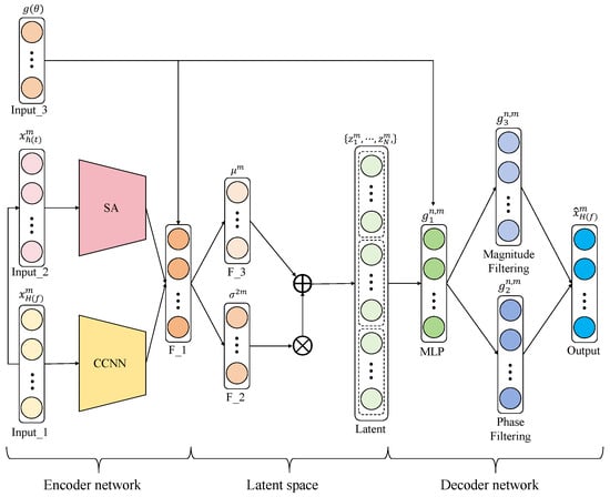
Figure 1. The complete training procedure of the PI-CVAE.

4.1. Time-Frequency Dual-Branch Encoding Framework

Structural dynamic responses show complex coupling between time and frequency, meaning that transient features and spectral properties are closely related. Because of this, the use of only frequency-domain analysis cannot capture transient dynamics, while using only time-domain modeling leads to unclear spectral information. To address this issue, the PI-CVAE uses a new dual-branch encoder that works in both the time and frequency domains. This architecture extracts and combines temporal and spectral features at the same time, creating a unified representation that is more consistent with physical laws. The time-domain branch extracts transient features like signal decay rates. These rates are closely related to frequency-domain properties, including structural damping ratios and half-power bandwidths.

The input to the time-domain branch is the Impulse Response Function (IRF), which is obtained by applying the Inverse Discrete Fourier Transform (IDFT) to the complex-valued Frequency Response Function (FRF):

$$h\left[n\right]={\mathcal{F}}^{-1}\left\{H\left(f\right)\right\}={\displaystyle \frac{1}{N}}\sum _{k=0}^{N-1}H\left[k\right]e^{j2\pi kn/N},n=0,1,\dots ,N-1$$

Before transformation, the FRF undergoes preprocessing to obtain a physically admissible and causal impulse response. Conjugate symmetry is enforced in the frequency domain to guarantee a real-valued time signal. A frequency-domain window is applied to mitigate artifacts induced by the finite spectral representation. Subsequently, a temporal alignment is performed by shifting all impulse responses such that their primary peaks coincide, thereby establishing a consistent temporal reference for the subsequent neural network processing. This preprocessing pipeline ensures that the extracted time-domain features are physically consistent and directly comparable across samples.

This branch processes the discrete-time response signal ($h\left[n\right]\in {\mathbb{R}}^T(n=0,\cdots ,T-1)$) through a causal convolutional neural network. The operation at layer m is defined as follows:

$$h\left[n\right]\left[m\right]=\sigma \sum _{i=0}^{k-1}W\left[i\right]\left[m\right]h[n-i][m-1]+b\left[m\right]$$

(4)

where $W\left[m\right]\in {\mathbb{R}}^{k\times d_{in}\times d_{out}}$ is a learnable convolution kernel. The causality constraint $(n-i\ge 0)$ ensures that the output at each time step (n) relies only on the current and past inputs ($h[n-i]$), preventing the use of any future information $(n-i<0)$.

The final feature vector (${\mathbf{z}}_t$) is obtained by flattening the output of the last convolutional layer ($h^{\left[L\right]}$).

$${\mathbf{z}}_t=\mathrm{Flatten}\left(h^{\left[L\right]}\right)\in {\mathbb{R}}^{D_t},$$

(5)

where L denotes the total number of layers and $D_t$ is the flattened dimension. This vector captures the essential temporal decay characteristics of the dynamic response.

The frequency-domain branch employs a specialized self-attention mechanism to identify and prioritize resonant modes. Conventional self-attention uses shared linear projections to generate the Query (Q), Key (K), and Value (V) matrices, which limits its ability to concurrently capture both localized resonance bands and global spectral interactions in structural dynamic responses. In the PI-CVAE, a hybrid projection strategy generates the three matrices (Q, K, and V) through separate, physics-guided pathways. This design tailors each matrix for a distinct physical role, thereby enhancing the differentiation of extracted features.

The Query matrix (Q) is designed to identify local spectral features near potential resonance peaks. It is produced by applying a 1D convolution operation to the input frequency spectrum ($X=\left|H\right(f\left)\right|$):

$$Q=LeakyReLU\left(Conv1D(X;W_q)\right)\in {\mathbb{R}}^{F\times d_k}$$

(6)

where $W_q\in {\mathbb{R}}^{m\times d_k}$ represents the learnable kernel weight.

The convolutional kernel width (m) is set to a fixed value, chosen to correspond to the typical half-power bandwidth ($\Delta f$) expected in structural dynamic systems.

This ensures the convolution covers a frequency range that matches the resonance bandwidth. Symmetric padding is applied to preserve information at the spectral boundaries. In addition, LeakyReLU activation with a negative slope of 0.1 is used instead of ReLU to avoid the vanishing gradient problem. This is important for retaining information from small or negative pre-activations, which often represent physically meaningful but weak higher-order vibration modes.

The Key matrix (K) captures a global representation of the frequency spectrum. It is produced by processing the concatenated input ($[X;g(\mathit{\theta }\left)\right]$) through a Multi-Layer Perceptron (MLP).

$$K=W_2·\mathrm{Swish}(W_1[X;g(\mathit{\theta })]+b_1)+b_2$$

(7)

where $W_1$ and $W_2$ are learnable weight matrices and $b_1$ and $b_2$ are bias terms. Unlike the locally focused convolutional filter used for Q, the MLP inherently captures interactions across all frequency points. This allows it to effectively represent long-range dependencies and global modal couplings. The Swish activation function ($x·\sigma \left(x\right)$) is chosen for its beneficial traits, such as smoothness and non-monotonicity. These properties often lead to better performance and more stable gradients than ReLU. By explicitly incorporating the physical parameters ($\mathit{\theta }$), the network can dynamically adjust this global representation according to the specific structural configuration.

The Value matrix (V) contains the fundamental spectral information to be weighted and aggregated. It is formulated as an element-wise scaling of the input spectrum to preserve the intrinsic energy distribution of the original frequency response:

$$V=W_v\odot X$$

(8)

where $W_v\in {\mathbb{R}}^{F\times d_v}$ is a learnable weight matrix, ⊙ denotes the Hadamard (element-wise) product, and $X=\left|H\right(f\left)\right|$ is the input spectrum. This formulation is guided by the principle of energy conservation, as expressed by Parseval’s theorem:

$$\sum _t{\left|h\left(t\right)\right|}^2=\sum _f{\left|H\left(f\right)\right|}^2$$

(9)

By performing only element-wise scaling, the transformation preserves the intrinsic structure of the spectral energy distribution.

The fused frequency-domain feature (${\mathbf{z}}_f$) is then computed through an attention mechanism as a weighted sum of the Value matrix (V). The attention weights ($\alpha \left(f\right)$) are obtained by comparing the locally focused Query vectors (Q) with the globally informed Key vectors (K):

$$\alpha \left(f\right)=\mathrm{Softmax}\left({\displaystyle \frac{Q{K}^T}{\sqrt{d}}}\right)$$

(10)

$${\mathbf{z}}_f=\alpha V$$

(11)

This mechanism enables the model to dynamically amplify or attenuate specific frequency components according to their physical significance.

The time-domain feature (${\mathbf{z}}_f$) and frequency-domain feature (${\mathbf{z}}_t$), which are outputs of the dual-branch encoder, are fused into a unified representation. This representation is then coupled with the underlying structural properties by incorporating the physical parameters ($\mathit{\theta }$) through an embedding network ($g(·)$). The complete fused feature vector is constructed using the following equation.

$${\mathbf{z}}_{\mathrm{fused}}=[{\mathbf{z}}_f;{\mathbf{z}}_t]+g(\mathit{\theta })$$

(12)

The fused feature vector (${\mathbf{z}}_{\mathrm{fused}}$) is projected by the encoder to obtain the parameters of the latent distribution.

Two separate linear layers are used to output the mean (${\mu }_{\varphi }$) and the log variance ($log{\sigma }_{\varphi }^2$) of the distribution. The latent variable ($\mathbf{z}$) is sampled via the reparameterization trick, expressed as

$$z={\mu }_{\varphi }+{\sigma }_{\varphi }\odot ϵ,ϵ\sim \mathcal{N}(0,I),$$

(13)

which enables gradient-based optimization during training. This stochastic sampling introduces a probabilistic dimension to the encoding process, which is essential for supporting uncertainty quantification.

4.2. Learnable Frequency-Filtering Decoder Network

The decoder of the PI-CVAE employs a learnable frequency-filtering method to generate FRFs that are inherently regularized towards physical plausibility. While not imposing hard constraints internally, its design works synergistically with the physics-informed loss functions (Section 4.3) to ensure non-negative magnitudes, causal phase relationships, and realistic damping behavior in the final output. Specifically, the method decodes the latent variable ($\mathbf{z}$) and structural parameters ($\mathit{\theta }$) into a consistent FRF by dynamically adjusting the spectral amplitude and phase.

The initial FRF prediction module takes the concatenated input $[\mathbf{z};\mathit{\theta }]$ and processes it through an MLP to generate a preliminary, complex-valued estimate of the FRF across all frequency points (f):

$${\widehat{H}}_{\mathrm{raw}}\left(f\right)=\mathrm{MLP}\left([\mathbf{z};\mathit{\theta }]\right)\in {\mathbb{C}}^F$$

(14)

In practice, the MLP outputs a real-valued vector of dimension $2F$. The first F elements are interpreted as the real part ($\Re \left\{{\widehat{H}}_{\mathrm{raw}}\left(f\right)\right\}$), and the subsequent F elements as the imaginary part ($\Im \left\{{\widehat{H}}_{\mathrm{raw}}\left(f\right)\right\}$). This two-channel representation allows for the use of standard real-valued neural network frameworks. The complex-valued estimate is then reconstructed as follows:

$${\widehat{H}}_{\mathrm{raw}}\left(f\right)=\Re \left\{{\widehat{H}}_{\mathrm{raw}}\left(f\right)\right\}+j\Im \left\{{\widehat{H}}_{\mathrm{raw}}\left(f\right)\right\}.$$

The initial phase ($\angle {\widehat{H}}_{\mathrm{raw}}\left(f\right)$) is directly computed from this complex representation via the arctangent function $(\angle {\widehat{H}}_{\mathrm{raw}}\left(f\right)=atan2(\Im \left\{{\widehat{H}}_{\mathrm{raw}}\left(f\right)\right\},\Re \left\{{\widehat{H}}_{\mathrm{raw}}\left(f\right)\right\})$, ensuring mathematical consistency. The subsequent phase correction ($\beta \left(f\right)$; Equation (16)) is applied to this initial phase as an additive term.

The amplitude processing component applies a frequency-dependent filter to enforce the non-negativity of the generated FRF magnitude. This constraint is implemented via a sigmoid-activated transformation, expressed as

$$A\left(f\right)=\sigma ({\mathbf{W}}_a\mathbf{z}+{\mathbf{b}}_a)\in {[0,1]}^F,$$

(15)

where ${\mathbf{W}}_a\in {\mathbb{R}}^{F\times k}$ is a learnable weight matrix that captures frequency-specific patterns and ${\mathbf{b}}_a$ is a bias term that sets baseline attenuation levels.

The sigmoid function is well-suited for this task. Its output is naturally bounded between 0 and 1, which guarantees non-negative magnitudes. Furthermore, its smooth gradient and asymptotic saturation support stable training and resemble the finite energy dissipation seen in real structures.

In parallel with the amplitude processing, the phase component ensures that the generated FRF exhibits causal and physically realistic phase behavior. It computes a phase correction term ($\beta \left(f\right)$) using a hyperbolic tangent (tanh) transformation:

$$\beta \left(f\right)=\pi ·\tanh ({\mathbf{W}}_b\mathbf{z}+{\mathbf{b}}_b)\in {[-\pi ,\pi ]}^F$$

(16)

where ${\mathbf{W}}_b$ learns to modulate the phase dynamically and ${\mathbf{b}}_b$ provides a baseline phase offset.

Bounding the phase within this interval is a processing step that is necessary to prevent phase wrapping and achieve alignment with the range of the principal value of the argument. It should be noted that while this constraint is necessary for a causal response, it is not sufficient by itself to guarantee strict causality, which requires the full Kramers–Kronig relations between the real and imaginary parts of the FRF to be satisfied. In the proposed framework, the overall physical consistency and causality of the generated FRF emerge from the synergistic effect of multiple mechanisms: the non-negativity constraint on the magnitude; the guidance provided by the physics-informed loss functions; and the fact that the model is trained on data originating from physically realizable, causal systems.

The physically consistent $\widehat{H}\left(f\right)$ is obtained by applying the adaptive amplitude filter ($A\left(f\right)$) and phase correction ($\beta \left(f\right)$) to the initial raw estimate (${\widehat{H}}_{\mathrm{raw}}\left(f\right)$). This synthesis process is mathematically described by the following equation.

$$\widehat{H}\left(f\right)=A\left(f\right)\odot \left|{\widehat{H}}_{\mathrm{raw}}\left(f\right)\right|\odot e^{j(\angle {\widehat{H}}_{\mathrm{raw}}\left(f\right)+\beta \left(f\right))}$$

(17)

where ⊙ represents the Hadamard (element-wise) product.

This operation ensures physical consistency via two key mechanisms. First, the magnitude spectrum is dynamically scaled by the sigmoid-constrained amplitude filter ($A\left(f\right)$), which suppresses non-physical resonance peaks and enforces non-negative energy values. Second, the phase spectrum is adjusted by the tanh-bounded correction term ($\beta \left(f\right)$) to maintain a causal and realistic waveform. Together, these operations effectively prevent the generation of non-physical spectra.

4.3. Physical Losses

Conventional loss functions for the training of a standard variational autoencoder combine a reconstruction loss ($\mathcal{L}\mathrm{recon}$) and a latent regularization term ($\mathcal{L}\mathrm{reg}$). The standard objective (${\mathcal{L}}_{\mathrm{CVAE}}$) is formulated as

$${\mathcal{L}}_{\mathrm{CVAE}}={\mathcal{L}}_{\mathrm{recon}}+{\mathcal{L}}_{\mathrm{reg}},$$

(18)

The first term (${\mathcal{L}}_{\mathrm{recon}}=\mathbb{E}[log{p}_{\psi }\left(\mathbf{H}\right|\mathbf{z},\mathit{\theta })]$) encourages accurate data reconstruction, often implemented as the Mean Squared Error (MSE). The second term (${\mathcal{L}}_{\mathrm{reg}}=D_{KL}(q_{\varphi }\left(\mathbf{z}\right|\mathbf{H},\mathit{\theta })\Vert p\left(\mathbf{z}\right))$) regularizes the latent space distribution ($q_{\varphi }$) towards a prior ($p\left(\mathbf{z}\right)=\mathcal{N}(\mathbf{0},\mathbf{I})$).

While these terms ensure probabilistic modeling and data fidelity, they often fail to enforce basic structural dynamics principles. The generated responses may exhibit non-physical artifacts, such as inaccurate resonance frequencies or unrealistic damping behavior.

To address these issues, the PI-CVAE framework introduces a comprehensive physics-informed loss system. This system includes a temporal decay-rate loss to maintain realistic damping behavior and a spectral peak alignment loss to correctly identify resonance frequencies. This multi-objective strategy balances accuracy relative to training data with consistency with physical laws.

The envelope of a signal, representing its time-varying amplitude, is extracted using the Hilbert transform. For the target signal ($h\left(t\right)$) and the generated signal ($\widehat{h}\left(t\right)$), the envelopes ($A\left(t\right)$ and $\widehat{A}\left(t\right)$) are obtained as follows:

$$A\left(t\right)=|h\left(t\right)+j·\mathcal{H}\left\{h\left(t\right)\right\}|,\widehat{A}\left(t\right)=|\widehat{h}\left(t\right)+j·\mathcal{H}\left\{\widehat{h}\left(t\right)\right\}|,$$

(19)

where $\mathcal{H}$ denotes the Hilbert transform operator. The formulation of this loss is motivated by the energy dissipation characteristics of dynamic systems. In a viscously damped system undergoing free decay, the envelope decays exponentially, leading to a linear decrease in the logarithmic envelope with a slope proportional to the damping. While the impulse responses processed here are not necessarily free decays, their envelopes inherently reflect the system’s energy dissipation properties. Therefore, comparison of the derivatives of the logarithmic envelopes provides a sensitive measure of whether the generated response captures the correct damping trends. Thus, the decay-rate loss is defined as the mean squared error between the following derivatives:

$${\mathcal{L}}_{\mathrm{decay}}={\displaystyle \frac{1}{T}}{\int }_0^T{\left({\displaystyle \frac{d}{dt}}lnA\left(t\right)-{\displaystyle \frac{d}{dt}}ln\widehat{A}\left(t\right)\right)}^{2}dt.$$

(20)

This loss term acts not as a strict enforcer of a single-degree-of-freedom exponential decay model but, rather, as a physics-informed regularizer. It penalizes deviations from a broadly monotonic and physically reasonable decay pattern, thereby encouraging the generative model to respect the fundamental principle of energy dissipation observed in real structural systems.

The spectral peak alignment loss (${\mathcal{L}}_{\mathrm{peak}}$) ensures accurate localization by minimizing the difference between the peaks in the true and generated frequency response functions. The resonance peaks are identified from both the true FRF ($\left|H\right(\omega \left)\right|$) and the generated FRF ($|\widehat{H}\left(\omega \right)|$) as all local maxima that meet the following condition.

$${\Omega }_{\mathrm{real}}=\left\{{\omega }_i|{\displaystyle \frac{d\left|H\right({\omega }_i\left)\right|}{d\omega }}=0, {\displaystyle \frac{d^2\left|H\left({\omega }_i\right)\right|}{d{\omega }^2}}<0\right\}$$

(21)

$${\Omega }_{\mathrm{gen}}=\left\{{\omega }_i|{\displaystyle \frac{d|\widehat{H}\left({\omega }_i\right)|}{d\omega }}=0, {\displaystyle \frac{d^2\left|\widehat{H}\left({\omega }_i\right)\right|}{d{\omega }^2}}<0\right\}.$$

(22)

For each true resonance peak frequency (${\omega }_i\in {\Omega }_{\mathrm{real}}$), the frequency error ($\Delta {\omega }_i$) is calculated as the minimum distance to any generated resonance peak in ${\Omega }_{\mathrm{gen}}$.

$$\Delta {\omega }_i=\underset{j}{\min }|{\omega }_i-{\widehat{\omega }}_j|$$

(23)

To handle outliers and potential mismatches in the number of peaks in a robust way, the aggregate loss is computed with the Huber loss function, which is less sensitive to large errors than the mean squared error. The loss is defined as

$${\mathcal{L}}_{peak}={\displaystyle \frac{1}{N}}\sum _{i=1}^N\left\{\begin{array}{c}{\displaystyle \frac{1}{2}}\Delta {\omega }_i^{2}if\Delta {\omega }_i\le \delta ,\hfill \\ \delta (\Delta {\omega }_i-{\displaystyle \frac{1}{2}}\delta )otherwise,\hfill \end{array}\right.$$

(24)

where the threshold ($\delta$) is set to $2\Delta f$, with $\Delta f$ being the frequency resolution. This defines a reasonable error tolerance for peak alignment.

To ensure practical applicability, the peak alignment loss incorporates specific design choices that address robustness concerns inherent to frequency-domain analysis. The selection of the Huber loss function mitigates sensitivity to outliers, providing a balanced response to both small alignment errors and larger discrepancies that may arise from noise or imperfect peak detection. The matching criterion associates each ground-truth peak with its nearest counterpart in the generated spectrum. This approach inherently accommodates discrepancies in the number of identified peaks between the target and generated FRFs, preventing loss divergence while maintaining focus on the alignment of dominant spectral features. Furthermore, a threshold parameter of $\delta =2\Delta f$ is established with physical justification: it defines an acceptable alignment tolerance proportional to the frequency resolution ($\Delta f$). The factor of two represents a conservative engineering margin that acknowledges inherent limitations in frequency discretization while avoiding excessive tolerance that could compromise alignment accuracy.

The overall training objective for the PI-CVAE combines data reconstruction accuracy with the proposed physics-informed constraints and the inherent variational regularization term, expressed as

$${\mathcal{L}}_{\mathrm{total}}={\mathcal{L}}_{\mathrm{recon}}+{\mathcal{L}}_{\mathrm{reg}}+{\Lambda }_1{\mathcal{L}}_{\mathrm{peak}}+{\Lambda }_2{\mathcal{L}}_{\mathrm{decay}}.$$

(25)

The weighting coefficients (${\Lambda }_1$ and ${\Lambda }_2$) follow a linear warm-up schedule. Their values increase linearly from 0 to their final magnitudes (0.1 and 0.05, respectively) over the first 80% of the training epochs. This curriculum allows the model to first stabilize with the standard CVAE objective (${\mathcal{L}}_{\mathrm{recon}}+{\mathcal{L}}_{\mathrm{reg}}$) before gradually enforcing the physics-informed constraints. This balances the influence of each constraint, promotes stable optimization, and prevents any single loss term from dominating the gradient updates.

This multi-component loss function enables the model to concurrently achieve high data accuracy, physically realistic dynamic behavior, and a well-organized latent space that supports effective uncertainty propagation.

4.4. Uncertainty Propagation Analysis

The trained PI-CVAE model facilitates highly efficient uncertainty propagation analysis by acting as a fast replacement for computationally expensive finite element simulations during Monte Carlo sampling. The overall procedure is divided into two sequential stages, including an offline training phase and an online propagation phase.

The initial offline phase represents a one-time computational investment for model development. This process starts with the creation of a training dataset. A set of N input parameter vectors (${\left\{{\mathit{\theta }}_i\right\}}_{i=1}^N$) is generated through Latin Hypercube Sampling (LHS) to uniformly explore the parameter space. For each parameter vector, a high-fidelity finite element simulation computes the corresponding frequency response function (${\mathbf{H}}_i$).

This set of parameter–FRF pairs ($\mathcal{D}={\{{\mathit{\theta }}_i,{\mathbf{H}}_i\}}_{i=1}^N$) forms the training dataset for the PI-CVAE model.

After the offline training phase concludes, the online propagation phase begins. This phase uses the trained model to perform highly efficient uncertainty quantification. It starts by drawing a large number of samples (S) from the prior distribution of the input parameters ($p(\mathit{\theta })$). Generating a corresponding ${\widehat{\mathbf{H}}}^{\left(s\right)}$ for each parameter sample (${\mathit{\theta }}^{\left(s\right)}$) involves two steps. First, a latent variable is sampled from the prior (${\mathbf{z}}^{\left(s\right)}\sim p\left(\mathbf{z}\right)=\mathcal{N}(\mathbf{0},\mathbf{I})$). Then, the decoder deterministically maps the pair $({\mathbf{z}}^{\left(s\right)},{\mathit{\theta }}^{\left(s\right)})$ to the output (${\widehat{\mathbf{H}}}^{\left(s\right)}={\mathrm{Decoder}}_{\mathit{\theta }}({\mathbf{z}}^{\left(s\right)},{\mathit{\theta }}^{\left(s\right)})$). The computational advantage of the method stems from this sub-millisecond generation capability. The resulting set of generated FRFs forms a Monte Carlo estimate of the full predictive distribution. Key statistical moments, such as the mean and standard deviation of the response, can then be directly computed from this ensemble for comprehensive uncertainty analysis.

5. Numerical Verifications

This section numerically validates the proposed PI-CVAE framework for uncertainty propagation in structural dynamics, assessing its accuracy, efficiency, and generalizability.

To guarantee an unbiased assessment and prevent data leakage, a rigorous data separation protocol was employed. For each structure, the dataset was partitioned into three distinct subsets. The training set comprised 100 parameter vectors generated via Latin Hypercube Sampling (LHS) to ensure space-filling coverage of the input domain. A separate validation set of 25 LHS samples was used exclusively for hyperparameter tuning and early stopping. The independent test set consisted of 2000 samples drawn via Monte Carlo sampling from the prior parameter distribution and was entirely disjoint from the training and validation data. All models, including the proposed PI-CVAE and the benchmark surrogates, were trained solely on the training set. All performance metrics reported in this section—the coefficient of determination ($R^2$), maximum FRF error, and ensemble statistics—were calculated exclusively on the held-out test set. This protocol ensures that the reported results reflect true generalization performance.

For a fair comparison, the framework is benchmarked against several established surrogates, including fifth-order Polynomial Chaos Expansion (PCE), Gaussian Process (GP) regression with a Matérn kernel, a standard CVAE, and Physics-Informed Neural Networks (PINNs).

5.1. Cantilever Plate

The cantilever plate serves as a benchmark to evaluate the PI-CVAE framework. The model is tested first on in-domain parameter variations to measure accuracy and efficiency, then on extrapolated parameter ranges to assess its generalization ability. Finally, the model is compared with established surrogate modeling techniques, showing its usefulness for uncertainty propagation in structural dynamics.

This case study uses a standard cantilever plate with the parameters shown in Figure 2 and Table 2. Three parameters—thickness (h), Young’s modulus (E), and mass density ($\rho$)—are modeled as Gaussian variables to represent manufacturing uncertainties. Two variation levels are defined in Table 3. Case I (COV 1–5%) tests performance within the training domain, while Case II (COV 3–10%) evaluates generalization beyond trained parameters. This approach assesses both interpolation and extrapolation capability. The training data contain 100 samples generated via Latin hypercube sampling using Case I parameter ranges.

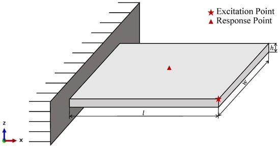
Figure 2. Geometric model of the cantilever plate.

Table 2. Material and geometric parameters of the plate.

Parameter	Value
Length (L)	370 mm
Width (B)	280 mm
Thickness (h)	2.5 mm
Mass density ($\rho$)	2750 kg/m3
Poison’s ratio ($\mu$)	0.33
Young’s modulus (E)	68.9 GPa

Table 3. Variability of input variables in uncertainty analysis for the cantilever plate.

Selected Parameter	Thickness (h)	Young’s Modulus (E)	Mass Density ($\mathit{\rho }$)
COV (Case I)	1%	5%	5%
COV (Case II)	3%	10%	10%

Standard convergence is observed for the cantilever plate under Case I, as shown in Figure 3a. Oscillatory behavior is exhibited during extrapolation to Case II, which demonstrates the robustness of the model to distribution shifts, as illustrated in Figure 3b.

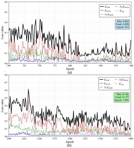
Figure 3. Convergence of the training loss for the PI-CVAE model in the case of the cantilever plate. (a) Case I; (b) Case II.

Ten randomly selected FRF curves from both PI-CVAE predictions and high-fidelity finite element references are compared in Figure 4. The curves match closely across the entire frequency range, including key resonance regions.

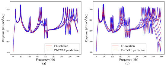
Figure 4. Acceleration FRFs of the cantilever plate from the PI-CVAE model (red solid lines) versus the FE solutions (blue dotted lines) at 10 test sample points.(a) Case I; (b) Case II.

The accelerance FRF ensembles from 2000 Monte Carlo samples generated by the PI-CVAE surrogate and high-fidelity finite element references are compared in Figure 5a,b. The results show close agreement across the frequency range, with the surrogate accurately capturing amplitude variations, stochastic spread, and sharp resonance peaks. The close match between the mean FRF from the PI-CVAE and the FE reference is shown in Figure 5c, where random variations are effectively smoothed to produce an unbiased estimate. The standard deviation, which quantifies response dispersion due to input uncertainty, is accurately reproduced, as evidenced in Figure 5d. Having established its in-domain accuracy, we proceed to assess the model’s performance under the extrapolative conditions of Case II.

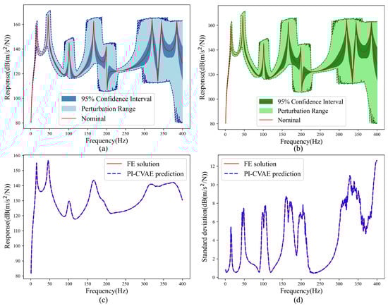
Figure 5. Acceleration FRFs of the cantilever plate predicted by the PI-CVAE model versus the FE model evaluated for 2000 MC samples for Case I. (a) PI-CVAE model prediction based on MC; (b) FE solution based on MC; (c) mean of FRFs; (d) standard deviation of FRFs.

In this test, the same PI-CVAE model trained on Case I is applied without any modification to predict responses for the much wider uncertainties in Case II. Even with the large change in input parameters, the FRF ensembles from the PI-CVAE (Figure 6a) still match the FE references (Figure 6b) very well. The model correctly captures the resulting shifts in resonance frequencies and the greater amplitude variability. The mean and standard deviation for Case II are accurately reproduced by the model, as shown in Figure 6c,d, indicating its correct capture of the increased response variability resulting from larger input uncertainties.

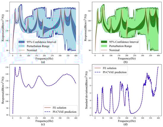
Figure 6. Acceleration FRFs of the cantilever plate predicted by the PI-CVAE model versus the FE model evaluated for 2000 MC samples for Case II. (a) PI-CVAE model prediction based on MC; (b) FE solution based on MC; (c) mean of FRFs; (d) standard deviation of FRFs.

The distribution of pointwise FRF errors for this case is presented in Figure 7a, where most errors are below 0.1%, with a maximum error of 0.12%. This low error level confirms the model’s high numerical accuracy and its ability to learn from limited data. For Case II, the error distribution remains similarly low (Figure 7b). The maximum error increases only slightly to 0.15%, showing minimal accuracy loss, even far beyond the training range. This stability results from the physics-informed architecture, which restricts solutions to physically realistic ranges.

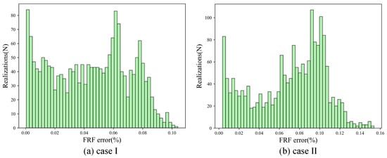
Figure 7. Histograms of the FRF prediction error by the PI-CVAE model for the cantilever plate across 2000 MC samples. (a) Case I; (b) Case II.

A comparison between PI-CVAE and established surrogate models for the case of the cantilever plate is provided in Table 4. PI-CVAE achieves significantly higher accuracy, with errors one to two orders of magnitude lower than PCE and GP. Unlike PCE, it avoids non-physical resonance peaks due to its physics-informed architecture. Under extrapolation (Case II), the accuracy advantage of PI-CVAE is greater. PCE and GP errors rise sharply to 23% and 12%, while PI-CVAE maintains minimal error (0.12% to 0.15%). PI-CVAE balances CVAE’s data efficiency with PINNs’ physical consistency, achieving superior accuracy without additional training data. A single high-fidelity FE simulation for this case takes 42.7 s. The complete PI-CVAE workflow requires about 2.9 h in total for data generation, training, and prediction. This represents a net speedup exceeding 8× over the 23.7 h needed for a direct 2000-sample Monte Carlo analysis.

Table 4. Comprehensive performance comparison for the cantilever-plate case study.

Method	PCE	GP	CVAE	PINN	PI-CVAE (Proposed)
Case I: Interpolation (COV 1–5%)
Max FRF Error	8.53%	6.21%	4.84%	3.11%	0.12%
R2	0.85	0.92	0.94	0.96	0.998
Case II: Extrapolation (COV 3–10%)
Max FRF Error	23.54%	12.25%	7.78%	5.21%	0.15%
R2	0.69	0.81	0.92	0.93	0.996
Efficiency
Training Duration (min)	25.8	35.4	52.1	68.9	85.3
Single Prediction (ms)	132.6	623.8	258.4	382.1	488.7

The cantilever-plate study definitively demonstrates the PI-CVAE framework’s high accuracy and robustness for uncertainty propagation, both within and beyond its training domain. As a fundamental validation measure, these results provide substantial evidence regarding the model’s capacity and establish a foundational basis for the investigation of more intricate structural systems.

5.2. T-Shaped Plate

This case study employs a T-shaped welded plate to further evaluate the framework’s robustness and general applicability. This structure contains geometric discontinuities that produce complex dynamic behavior.

The geometry and material properties of the asymmetric T-shaped plate are depicted in Figure 8 and summarized in Table 5. The test setup excites the center point of the left flange and measures the response at the center point of the right flange. Uncertainties in thickness, Young’s modulus, and mass density are modeled as independent Gaussian variables with a 3% coefficient of variation. These parameters vary uniformly across all structural components. Specifically, the plate is divided into four regions for parameter perturbation: the left flange, right flange, upper plate, and welded joint.

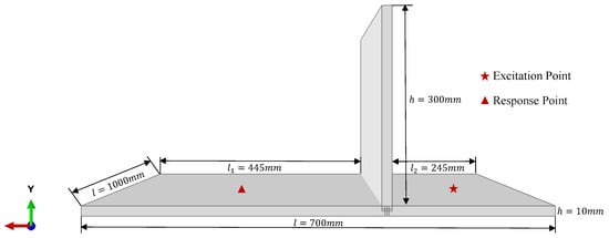
Figure 8. Geometric model of the asymmetric T-shaped plate.

Table 5. Material and geometric parameters of the T-shaped plate.

Parameter	Value
Mass density ($\rho$)	7850 kg/m3
Poison’s ratio ($\mu$)	0.28
Young’s modulus (E)	205 GPa

A final loss of 0.12–0.18 is achieved by PI-CVAE, despite slower convergence, as illustrated in Figure 9.

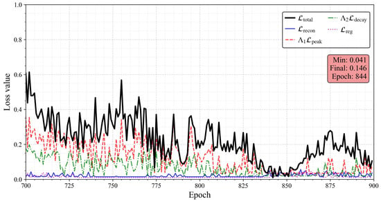
Figure 9. Convergence of the training loss for the PI-CVAE model in the case of a T-shaped plate.

Close agreement between predicted and reference responses is observed across ten sample FRF realizations, which are compared in Figure 10.

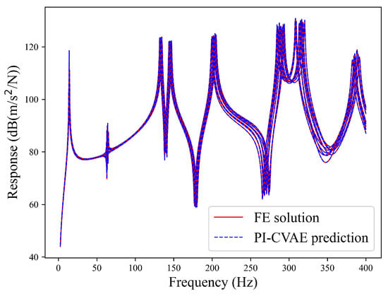
Figure 10. Acceleration FRFs of the T-shaped plate from the PI-CVAE model (red solid lines) versus the FE solutions (blue dotted lines) at 10 test sample points.

High accuracy is observed in the matching between the FRF ensembles and the FE references, as shown in Figure 11a,b, where closely spaced and higher-order modes are captured, despite geometric discontinuities. The model also precisely reproduces both the mean response in Figure 11c and the standard deviation in Figure 11d.

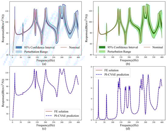
Figure 11. Acceleration FRFs of the T-shaped plate predicted by the PI-CVAE model versus the FE model evaluated for 2000 MC samples. (a) PI-CVAE model prediction based on MC; (b) FE solution based on MC; (c) mean of FRFs; (d) standard deviation of FRFs.

The distribution of prediction errors across all frequencies is presented in Figure 12. The errors remain very low, confirming the model’s high accuracy.

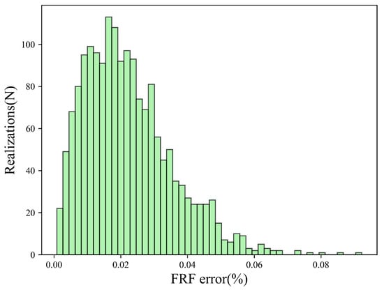
Figure 12. Histograms of the FRF prediction error by the PI-CVAE model for the T-shaped plate across 2000 MC samples.

A comparison of model performance for the T-shaped plate is provided in Table 6, which shows that PI-CVAE achieves the highest accuracy, with a minimal prediction error of 0.085%, significantly outperforming conventional methods. The framework also provides major computational savings. Each FE evaluation for the T-shaped plate requires 83.4 s. The full PI-CVAE procedure completes a 2000-sample uncertainty quantification in approximately 4.1 h, achieving an overall acceleration of over 11 times compared to a direct Monte Carlo FE simulation, which would take about 46.3 h.

Table 6. Variability of input variables in uncertainty analysis for T-shaped plate.

Method	PCE	GP	CVAE	PINN	PI-CVAE (Proposed)
Max FRF Error	8.08%	5.21%	4.98%	1.98%	0.085%
R2	0.82	0.90	0.91	0.94	0.992
Training Duration (min)	28.5	42.7	68.3	72.6	88.4
Single Prediction (ms)	158.9	735.2	312.6	458.3	582.1

Validation with a T-shaped plate confirms that the PI-CVAE framework effectively handles geometric discontinuities and local stiffness changes. With prediction times under one second, this approach enables previously unfeasible uncertainty analysis for complex structures. These capabilities make PI-CVAE suitable for industrial use. It meets the dual requirements of accuracy and speed when applied to complex geometries.

5.3. Ablation Study

This section presents an ablation study to quantify the contributions of key components within the PI-CVAE architecture. This analysis isolates the physics-informed modules to evaluate their necessity beyond conventional performance metrics. The study uses a cantilever plate under Case I conditions, with model variants assessed through numerical accuracy and physical plausibility metrics. The following variants were created by removing or replacing specific components in the full model.

• Full PI-CVAE: The complete proposed model;
• w/o Time Branch: Removes the time-domain causal convolutional branch;
• w/o Frequency Branch: Removes the frequency-domain self-attention branch;
• w/o Physics Losses: Removes the physics-informed loss terms (${\mathcal{L}}_{peak}$, ${\mathcal{L}}_{decay}$, and ${\mathcal{L}}_{reg}$), training the model solely on the reconstruction loss;
• w/o Frequency Filtering: Replaces the learnable frequency-filtering decoder with a standard MLP decoder.

Three complementary metrics are employed to provide a comprehensive assessment of the physical consistency and accuracy of the generated frequency response functions. All metrics are calculated exclusively on the held-out test set to ensure an unbiased evaluation.

Modal-frequency mean absolute error is used to quantify the accuracy of resonance frequency prediction. For each successfully matched resonance peak between the true and generated FRFs, the absolute difference in frequency is computed. The average across all matched peaks is reported. This metric directly measures the precision in identifying the system’s eigenvalues and is defined as follows:

$${\mathrm{MAE}}_{\mathrm{freq}}={\displaystyle \frac{1}{N_{\mathrm{matched}}}}\sum _{i=1}^{N_{\mathrm{matched}}}\left|{\omega }_i^{\mathrm{true}}-{\omega }_i^{\mathrm{gen}}\right|.$$

The modal assurance criterion error evaluates the fidelity of the predicted mode shapes. The modal assurance criterion is computed for each pair of matched modes, with the mode shapes extracted from the corresponding columns of the FRF matrix at the matched resonance frequencies. The MAC value for a single mode pair is defined as follows:

$${\mathrm{MAC}}_i={\displaystyle \frac{{\left|{\left\{{\varphi }_i^{\mathrm{true}}\right\}}^H\left\{{\varphi }_i^{\mathrm{gen}}\right\}\right|}^2}{\left({\left\{{\varphi }_i^{\mathrm{true}}\right\}}^H\left\{{\varphi }_i^{\mathrm{true}}\right\}\right)\left({\left\{{\varphi }_i^{\mathrm{gen}}\right\}}^H\left\{{\varphi }_i^{\mathrm{gen}}\right\}\right)}},$$

where H denotes the Hermitian transpose. The overall MAC error is then calculated as $1-\overline{\mathrm{MAC}}$, where $\overline{\mathrm{MAC}}$ is the average MAC across all matched modes. A lower MAC error indicates better preservation of the modal shape information.

As shown in Table 7, noticeable degradations in both conventional accuracy (MAE and $R^2$) and physical consistency metrics (Modal Freq. MAE and MAC error) are observed when either the time- or frequency-domain branch is removed. Specifically, removing the time branch increases the Modal Freq. MAE from 0.8 Hz to 2.1 Hz and the MAC error from 0.02 to 0.12, while removing the frequency branch further degrades these metrics to 2.5 Hz and 0.15, respectively. This underscores the necessity of the dual-branch encoder for capturing coupled time-frequency physics. The variant without the learnable frequency-filtering decoder (w/o Frequency Filtering) shows a moderate increase in point-wise MAE (0.28%) but exhibits a substantial degradation in MAC error (0.21), confirming that the proposed decoder is essential for embedding physical constraints such as non-negativity and causal phase relationships directly into the generative process. The most severe physical violations are observed in the variant trained without physics-informed losses (w/o Physics Losses), which yields the highest MAC error (0.28) despite maintaining a relatively low Modal Freq. MAE (1.8 Hz). This demonstrates that while the model can achieve reasonable resonance-frequency localization, data-driven training alone cannot ensure physically consistent mode shapes and overall dynamic response fidelity.

Table 7. Ablation study results for the cantilever plate (Case I).

Model Variant	MAE (%)	${\mathit{R}}^2$	Modal Freq. MAE (Hz)	MAC Error
Full PI-CVAE	0.12	0.995	0.8	0.02
w/o Time Branch	0.31	0.96	2.1	0.12
w/o Frequency Branch	0.38	0.95	2.5	0.15
w/o Frequency Filtering	0.28	0.97	1.5	0.21
w/o Physics Losses	0.45	0.94	1.8	0.28

In summary, the ablation study demonstrates that the superior performance of the PI-CVAE stems from the synergistic integration of its three core components: the dual-branch encoder, physics-informed losses, and the frequency-filtering decoder. The removal of any single component leads to a measurable decline in either numerical accuracy or—more critically—the physical consistency of the generated responses.

6. Conclusions

The present work proposes a Physics-Informed Conditional Variational Autoencoder (PI-CVAE), a surrogate modeling strategy for efficient and physics-consistent uncertainty quantification of structural dynamic responses. Its major contribution lies in the integration of three components that address the specific demands of frequency response function generation: a dual-branch encoder for coupled time-frequency feature extraction, a learnable frequency-filtering decoder that ensures non-negative magnitudes and causal phase relationships, and a physics-informed loss function that prioritizes the statistical fidelity of interpretable engineering attributes. Comprehensive numerical validations demonstrate that the proposed approach maintains high accuracy while achieving significant computational speedup compared to conventional simulation techniques, establishing a practical and robust framework for uncertainty quantification in structural dynamics.

Comprehensive validation on cantilever and T-shaped plates confirms the PI-CVAE framework’s exceptional accuracy and robustness. The model achieves maximum FRF errors as low as 0.12% within the training domain and 0.15% under extrapolation, significantly outperforming conventional surrogate methods. With a computational speedup of 8–11× over direct Monte Carlo simulation and consistent generalization beyond trained parameter ranges, the framework demonstrates strong practicality for real-world uncertainty quantification in structural dynamics.

Future work will focus on enhancing the scalability of the framework for high-dimensional systems and extending it to quantify model-form uncertainties. These directions aim to further solidify PI-CVAE as an efficient and reliable tool for real-time reliability assessment and design optimization in aerospace, civil, and mechanical engineering applications.

References

- Soize, C. Stochastic modeling of uncertainties in computational structural dynamics—Recent theoretical advances. J. Sound Vib. 2013, 332, 2379–2395. [Google Scholar] [CrossRef]
- Schueller, G. On the treatment of uncertainties in structural mechanics and analysis. Comput. Struct. 2007, 85, 235–243. [Google Scholar] [CrossRef]
- Huang, B.; Ma, C.; Li, Y.; Wu, Z.; Zhang, H. Analytical approximation of dynamic responses of random parameter nonlinear systems based on stochastic perturbation-Galerkin method. Chaos Solitons Fractals 2024, 189, 115724. [Google Scholar] [CrossRef]
- Zhao, K.; Wu, F.; Wu, X.; Zhang, X.; Yang, Y. An adaptive high-order stochastic perturbation collocation method for uncertainty quantification and propagation. Appl. Math. Model. 2025, 146, 116185. [Google Scholar] [CrossRef]
- Kaminski, M.; Vaccaro, M.S.; Barretta, R. On a stochastic model of nonlocal elastic beams using the generalized perturbation method. Probabilistic Eng. Mech. 2025, 81, 3. [Google Scholar] [CrossRef]
- Śniady, P.; Adamowski, R.; Kogut, G.; Zielichowski-Haber, W. Spectral stochastic analysis of structures with uncertain parameters. Probabilistic Eng. Mech. 2008, 23, 76–83. [Google Scholar] [CrossRef]
- Chassaing, J.C.; Lucor, D.; Trégon, J. Stochastic nonlinear aeroelastic analysis of a supersonic lifting surface using an adaptive spectral method. J. Sound Vib. 2012, 331, 394–411. [Google Scholar] [CrossRef]
- Singh, B.; Bisht, A.; Pandit, M.; Shukla, K. Nonlinear free vibration analysis of composite plates with material uncertainties: A Monte Carlo simulation approach. J. Sound Vib. 2009, 324, 126–138. [Google Scholar] [CrossRef]
- Najm, H.N. Uncertainty quantification and polynomial chaos techniques in computational fluid dynamics. Annu. Rev. Fluid Mech. 2009, 41, 35–52. [Google Scholar] [CrossRef]
- Son, J.; Du, Y. An efficient polynomial chaos expansion method for uncertainty quantification in dynamic systems. Appl. Mech. 2021, 2, 460–481. [Google Scholar] [CrossRef]
- Xia, Z.; Tang, J. Characterization of dynamic response of structures with uncertainty by using Gaussian processes. J. Vib. Acoust. 2013, 135, 051006. [Google Scholar] [CrossRef]
- Li, M.J.; Lian, Y.; Cheng, Z.; Li, L.; Wang, Z.; Gao, R.; Fang, D. A clustering adaptive Gaussian process regression method: Response patterns based real-time prediction for nonlinear solid mechanics problems. Comput. Methods Appl. Mech. Eng. 2025, 436, 117669. [Google Scholar] [CrossRef]
- Nakarmi, S.; Leiding, J.A.; Lee, K.S.; Daphalapurkar, N.P. Predicting non-linear stress–strain response of mesostructured cellular materials using supervised autoencoder. Comput. Methods Appl. Mech. Eng. 2024, 432, 117372. [Google Scholar] [CrossRef]
- Lai, C.; Baraldi, P.; Zio, E. Physics-informed deep autoencoder for fault detection in new-design systems. Mech. Syst. Signal Process. 2024, 215, 111420. [Google Scholar] [CrossRef]
- Li, G.; Tang, L.; Sorokin, V.; Wang, S. CVAE-based inverse design of two-dimensional honeycomb pentamode metastructure for acoustic cloaking. Thin-Walled Struct. 2025, 206, 112623. [Google Scholar] [CrossRef]
- Steffensen, M.T.; Tcherniak, D.; Thomsen, J.J. Uncertainty in frequency response function estimates in experimental modal analysis. J. Sound Vib. 2025, 614, 119168. [Google Scholar] [CrossRef]
- Navarro, J.D.; Velasquez-Gonzalez, J.C.; Aristizabal, M.; Montoya, A.; Millwater, H.R.; Restrepo, D. Arbitrary-order sensitivity analysis of frequency response functions using hypercomplex automatic differentiation and spectral finite elements. Appl. Math. Comput. 2026, 510, 129677. [Google Scholar] [CrossRef]
- Jia, X.; Hou, W.; Cao, S.Z.; Yan, W.J.; Papadimitriou, C. Analytical hierarchical bayesian modeling framework for model updating and uncertainty propagation utilizing frequency response function data. Comput. Methods Appl. Mech. Eng. 2025, 447, 118341. [Google Scholar] [CrossRef]
- Ullah, A.; Yan, T.; Fuxin, L. CVAE-SM: A Conditional Variational Autoencoder with Style Modulation for Efficient Uncertainty Quantification. In 2024 IEEE International Conference on Robotics and Automation (ICRA); IEEE: Piscataway, NJ, USA, 2024; pp. 10786–10792. [Google Scholar]
- Shi, Y.; Wei, P.; Feng, K.; Feng, D.C.; Beer, M. A survey on machine learning approaches for uncertainty quantification of engineering systems. Mach. Learn. Comput. Sci. Eng. 2025, 1, 11. [Google Scholar] [CrossRef]
- Liang, D.; Yao, J.; Jia, Z.; Cao, Z.; Liu, X.; Jing, X. Novel neural network for predicting the vibration response of mistuned bladed disks. AIAA J. 2023, 61, 391–405. [Google Scholar] [CrossRef]
- Zhou, Z.; Gao, Y.; Cheng, Y.; Ma, Y.; Wen, X.; Sun, P.; Yu, P.; Hu, Z. Uncertainty quantification of vibroacoustics with deep neural networks and Catmull–Clark subdivision surfaces. Shock Vib. 2024, 2024, 7926619. [Google Scholar] [CrossRef]
- Raissi, M.; Perdikaris, P.; Karniadakis, G.E. Physics-informed neural networks: A deep learning framework for solving forward and inverse problems involving nonlinear partial differential equations. J. Comput. Phys. 2019, 378, 686–707. [Google Scholar] [CrossRef]
- Ju, L.; Zheng, Q.; Zhang, J.; Guo, S.; Chen, F. Estimating transient vertical hyporheic exchange fluxes from streambed temperatures using LSTM-autoencoder-enhanced physics-informed neural networks. J. Hydrol. 2025, 661, 133721. [Google Scholar] [CrossRef]
- Zideh, M.J.; Solanki, S.K. Multivariate physics-informed convolutional autoencoder for anomaly detection in power distribution systems with widespread deployment of distributed energy resources. Sustain. Energy Grids Netw. 2025, 44, 102022. [Google Scholar] [CrossRef]
- Wang, X.; Qian, W.; Zhao, T.; Chen, H.; He, L.; Sun, H.; Tian, Y. A generative design method of airfoil based on conditional variational autoencoder. Eng. Appl. Artif. Intell. 2025, 139, 109461. [Google Scholar] [CrossRef]
- Kim, Y.; Choi, Y.; Widemann, D.; Zohdi, T. A fast and accurate physics-informed neural network reduced order model with shallow masked autoencoder. J. Comput. Phys. 2022, 451, 110841. [Google Scholar] [CrossRef]
- Zhang, X.; Zhang, W.; Wen, S.; Ding, Q. Augmentation framework for HVAC fault diagnosis based on denoising diffusion models. J. Build. Eng. 2025, 106, 112646. [Google Scholar] [CrossRef]
- Li, G.; Zhan, L.; Fang, X.; Gao, J.; Xu, C.; He, X.; Deng, J.; Xiong, C. Performance comparison on improved data-driven building energy prediction under data shortage scenarios in four perspectives: Data generation, incremental learning, transfer learning, and physics-informed. Energy 2024, 312, 133640. [Google Scholar] [CrossRef]
- Chen, D.; Li, X.; Xu, J.; Wang, Z. An anomaly detection method for gas turbines in power plants using conditional variational autoencoder optimized with self-attention. Reliab. Eng. Syst. Saf. 2025, 267, 111894. [Google Scholar] [CrossRef]
- Glyn-Davies, A.; Duffin, C.; Akyildiz, O.D.; Girolami, M. Φ-DVAE: Physics-informed dynamical variational autoencoders for unstructured data assimilation. J. Comput. Phys. 2024, 515, 113293. [Google Scholar] [CrossRef]
- Wang, L.; Yang, M. Dual-Encoder Physics-Informed Variational Autoencoders for robust forward and inverse SDE solving under noisy measurements. Phys. A Stat. Mech. Its Appl. 2025, 679, 131008. [Google Scholar] [CrossRef]
- Gao, Z.; Yu, K.; Wu, J.; Jiang, W.; Yang, B. PET-AE: Physics-informed enhanced temporal autoencoder for incipient fault detection of shafting systems. Mech. Syst. Signal Process. 2025, 240, 113345. [Google Scholar] [CrossRef]
- Liu, J.; Li, C. Physics-informed tensor autoencoder with memory for video anomaly detection. Expert Syst. Appl. 2025, 298, 129576. [Google Scholar] [CrossRef]
- Zhuang, B.; Gallet, A.; Smyl, D. Inverse structural design with generative and probabilistic autoencoders and diffusion models. Eng. Appl. Artif. Intell. 2025, 161, 112143. [Google Scholar] [CrossRef]
- Rathnakumar, R.; Huang, J.; Yan, H.; Liu, Y. Bayesian Entropy Neural Networks for Physics-Aware Prediction. arXiv 2024, arXiv:2407.01015. [Google Scholar] [CrossRef]
- Pan, C.; Qiao, C.; Feng, S.; Li, Y.; Zheng, Y.; Ye, H. Robust measurement of surface tension and contact angle using physics-informed autoencoders. Colloids Surfaces A Physicochem. Eng. Asp. 2025, 730, 138972. [Google Scholar] [CrossRef]
- Zhang, C.; Zhao, Y.F. A hybrid deep learning approach for the design of 2D Auxetic Metamaterials. Comput. Methods Appl. Mech. Eng. 2025, 441, 117972. [Google Scholar] [CrossRef]
- Najera-Flores, D.A.; Qian, G.; Hu, Z.; Todd, M.D. Corrosion morphology prediction of civil infrastructure using a physics-constrained machine learning method. Mech. Syst. Signal Process. 2023, 200, 110515. [Google Scholar] [CrossRef]
- Shi, C.; Yin, C.; Luo, W.; Liu, H.; Tang, H. Study of current distribution generation in PEMFC based on Conditional Variational Auto-Encoder. Energy AI 2025, 21, 100568. [Google Scholar] [CrossRef]
- Xu, C.; Xu, C.; Sun, Y.; Chen, S.; Li, G. A physics-informed autoencoder method with automatic weighted loss for chiller water system sensor fault detection. Energy Build. 2025, 348, 116448. [Google Scholar] [CrossRef]
- Yue, K.; Li, Z.; Yao, X.; Du, W.; Yu, W.; Huang, W.; Wang, L. Physics-informed attention-aided multiple autoencoder for gear anomaly detection under zero-shot condition. Measurement 2025, 257, 118725. [Google Scholar] [CrossRef]
- Luo, K.; Zhao, J.; Wang, Y.; Li, J.; Wen, J.; Liang, J.; Soekmadji, H.; Liao, S. Physics-informed neural networks for PDE problems: A comprehensive review. Artif. Intell. Rev. 2025, 58, 323. [Google Scholar] [CrossRef]
- Klapa Antonion, X.W.; Raissi, M.; Joshie, L. Machine learning through physics–informed neural networks: Progress and challenges. Acad. J. Sci. Technol. 2024, 9, 46–49. [Google Scholar] [CrossRef]
- Booker, J.M.; Ross, T.J.; Reardon, B.J.; Hemez, F.M.; Anderson, M.C.; Doebling, S.W.; Joslyn, C.A. An Engineering Perspective on uq for Validation, Reliability and Certification. Foundations 2004. Available online: https://cliffjoslyn.github.io/Docs/BoJRoT04.pdf (accessed on 24 January 2026).
Disclaimer/Publisher’s Note: The statements, opinions and data contained in all publications are solely those of the individual author(s) and contributor(s) and not of MDPI and/or the editor(s). MDPI and/or the editor(s) disclaim responsibility for any injury to people or property resulting from any ideas, methods, instructions or products referred to in the content. |
© 2026 by the authors. Licensee MDPI, Basel, Switzerland. This article is an open access article distributed under the terms and conditions of the Creative Commons Attribution (CC BY) license.