Dynamic Temporal Network-Based Spatio-Temporal Evolution and Passenger Flow Prediction: A Case Study of Beijing Subway

Abstract

Against the backdrop of China’s “dual-carbon” goals, accurate analysis and prediction of subway passenger flows are crucial for optimizing operational efficiency and advancing low-carbon urban transportation. Beijing’s subway network exhibits pronounced spatiotemporal heterogeneity across workdays, weekends, and holidays, yet existing studies often rely on static networks or single-scale temporal analyses, failing to capture dynamic flow evolution. To address this gap, this study develops a dynamic time-varying network framework with a 15 min temporal granularity, integrating sliding time-window analysis, node strength evaluation, and betweenness centrality for bottleneck identification. A Temporal–Spatial Fusion Gated Recurrent Unit (TSF-GRU) model is proposed to fuse temporal dependencies, spatial correlations, and network topology for short-term passenger flow forecasting. Results show distinct flow patterns: workdays feature a “concentrated commuting” dual peak, holidays a “steady continuous” leisure pattern, and weekends an “extended flexible” hybrid pattern. Station functions and bottleneck evolution vary dynamically across date types, with transportation hubs central on holidays/weekends and business nodes dominating workday peaks. The TSF-GRU model achieves a test-set MAPE of 7.62% and bottleneck prediction accuracy of 92.3%, outperforming traditional methods. This study provides a feasible pathway for refined, low-carbon subway operations in megacities and methodological support for achieving dual-carbon goals.

1. Introduction

As China’s political, cultural, and international exchange center, as well as a highly developed megacity, Beijing exhibits diverse urban functions and a dense population, resulting in exceptionally high transportation demand—while also bearing the crucial task of advancing urban low-carbon transformation [1]. In the context of global efforts to mitigate climate change and China’s “dual carbon” (carbon peaking and carbon neutrality) goals, the development of public transportation, particularly rail transit, has become a core strategy for reducing urban carbon emissions. Since the inauguration of its first subway line in 1969, the Beijing Subway has undergone decades of development and expansion, evolving into a large-scale urban rail network characterized by extensive coverage, high line density, and strong transport capacity—and serving as a pivotal carrier of the city’s low-carbon travel system [2]. Currently, the Beijing Subway operates more than 20 lines with a total operational length exceeding 700 km [3]. This expansive network not only traverses core urban districts such as Dongcheng and Xicheng but also extends to suburban districts and counties including Tongzhou, Changping, and Daxing, creating an efficient transport framework that connects key urban areas while significantly reducing reliance on high-emission private vehicles [4,5]. As one of the busiest subway systems in the world, the Beijing Subway carries an immense daily passenger volume—its efficient operation directly translates to substantial carbon emission reductions by diverting traffic from road transport. During peak periods, multiple lines operate at high frequencies to meet passenger demand, further enhancing the substitution effect on private cars and consolidating the subway’s role in low-carbon urban mobility.

The spatiotemporal characteristics of Beijing Subway passenger flows are highly complex, with significant variations across different times of the day and pronounced fluctuations during holidays, major events, and other special circumstances. The passenger population is heterogeneous, including government employees, corporate staff, international residents, and students, with travel purposes ranging from commuting and shopping to entertainment and tourism [6]. Weekday peak periods are dominated by commuting flows—where subway travel achieves concentrated carbon reduction effects by replacing private car trips—whereas holiday periods see a predominance of tourism and shopping trips, requiring targeted scheduling to maintain low-carbon travel efficiency [7,8]. Therefore, an in-depth study of the dynamic characteristics of Beijing Subway passenger flows can not only accurately reveal the operational patterns of a megacity rail transit system but also provide critical support for optimizing the low-carbon performance of urban transportation. Such analysis offers scientific guidance for subway operators to optimize resource allocation—such as adjusting train frequency based on flow dynamics to avoid energy waste—and improve operational efficiency [9]. Additionally, it provides valuable support for urban traffic management, subway network planning and upgrades (e.g., extending lines to areas with high private car usage), and enhancement of passenger travel experiences—all of which contribute to boosting the attractiveness of public transportation and advancing the city’s low-carbon development goals, carrying significant theoretical and practical implications [10,11].

This study develops a generalizable framework for analyzing dynamic temporal subway networks. Unlike prior studies that often rely on coarse temporal intervals or static network representations, this framework constructs a high-resolution dynamic temporal network using a minute-level sliding window, capturing fine-grained spatiotemporal evolution of passenger flows across weekdays, weekends, and holidays. It further integrates network structure analysis, directional flow visualization, and bottleneck identification through node strength and betweenness centrality, while classifying key nodes into seven dynamic evolution patterns, allowing for a precise understanding of functional differentiation over time. Building on this, the study designs targeted management strategies and predictive models that directly link network insights to low-carbon operational efficiency, such as optimized train scheduling, resource allocation, and dynamic bottleneck management. While the Beijing Subway serves as a case study for validation, the methodology and analytical framework are transferable to other large-scale urban subway systems, offering a replicable approach for combining spatiotemporal passenger flow analysis, network topology evaluation, and sustainable, low-carbon urban transportation planning.

2. Literature Review and Research Contributions

This section systematically reviews the research progress in three key fields: spatiotemporal characteristics of subway passenger flow, subway network structure, and dynamic subway networks. It focuses on analyzing the limitations of current research—such as insufficient integration of low-carbon goals, coarse temporal granularity in dynamic network construction, and lack of dynamic differentiation analysis of node functions. On this basis, the research gaps addressed by this study, key contributions, and the overall structure of the paper are clarified, laying a theoretical foundation for subsequent methodological design and empirical analysis.

2.1. Research on Spatiotemporal Characteristics of Passenger Flow

Scholars have primarily relied on statistical analysis methods to study subway passenger flow spatiotemporal characteristics, processing volume data for specific periods to calculate metrics such as averages and peaks [12]. These metrics are then used to distinguish peak and off-peak periods and to identify basic differences in passenger distribution across different times. Some studies have further integrated spatial analysis, examining the distribution patterns of passenger flows across different areas, providing a foundation for understanding the spatiotemporal distribution of subway passenger flows [13]. However, few studies have linked these characteristics to low-carbon operational optimization, missing opportunities to tailor strategies for maximum emission reduction effects. In the field of network structure and node analysis, early research focused on static network topology, evaluating node importance using metrics such as degree, betweenness centrality, and closeness centrality, while analyzing network connectivity and robustness. With the progression of research, passenger flow data have increasingly been incorporated into assessments of node importance, constructing integrated frameworks that combine the physical network and passenger flow network to more accurately evaluate the significance of different subway stations [14,15].

Yet, the low-carbon value of node functions—such as how transport hubs or commercial stations contribute differently to emission reductions—remains underexplored, limiting the alignment of network optimization with carbon reduction targets. Regarding operational optimization, studies have focused on improving efficiency, reducing costs, and meeting passenger demand. Mathematical models and optimization algorithms, such as linear programming and genetic algorithms, have been applied to optimize parameters including train frequency, operation schedules, and station stops [16]. Some studies have also considered train delays and passenger flow uncertainties, developing stochastic programming models to enhance the robustness of operation plans, and have emphasized the integration of subway operations with other transport modes to promote coordinated optimization across the urban transport system [17]. However, these optimization efforts rarely prioritize carbon emission reduction as a core objective, leading to strategies that may improve efficiency but fail to maximize low-carbon benefits. At the level of passenger flow spatiotemporal analysis, existing research is largely constrained by static frameworks, which are insufficient for capturing the dynamic evolution of passenger flows over time. Consequently, these studies struggle to reveal the fundamental differences in passenger flow rhythms across weekdays, holidays, and weekends, and cannot accurately identify the intrinsic drivers of flow fluctuations—critical gaps for designing time-sensitive low-carbon strategies [18,19].

2.2. Research on Subway Network Structure

In network and node studies, there is insufficient attention to the dynamic differentiation of node functions, leaving the functional switching patterns of different station types across time periods underexplored. Additionally, node importance assessments often lack comprehensive multi-factor indicator systems that include low-carbon contribution, making it difficult to reflect the dynamic changes in node significance under varying spatiotemporal conditions [20]. In operational optimization practice, implementing optimization strategies faces multiple challenges [21,22]. Existing research has difficulty effectively coordinating train operations with station service capacity, lacks mature strategies for balancing operational cost control with passenger demand under dynamic flow conditions, and provides limited mechanisms for dynamically adjusting operation plans during emergencies [23]. Furthermore, there is insufficient analysis linking passenger flow characteristics with urban spatial functions and socioeconomic activity patterns—including their carbon emission implications—which limits the practical applicability of research findings for low-carbon urban governance.

In the field of subway network construction research, early traditional studies generally employed a static network construction approach [24,25,26]. These studies abstracted subway stations as nodes with only spatial attributes such as longitude and latitude, and defined a single passenger trip from an origin station to a destination station as a directed edge connecting two nodes, with a primary focus on analyzing the spatial topology of the network [27]. Using this static construction approach, scholars were able to preliminarily reveal fundamental characteristics of subway networks, such as connectivity and the distribution of node importance, providing an initial theoretical basis for network planning and layout [28,29]. The core advantages of this approach lie in its simplicity and computational convenience, allowing rapid visualization of the network’s static structural relationships.

2.3. Research on Dynamic Subway Networks

As research progressed, some scholars gradually recognized the crucial influence of the temporal dimension on subway network operations, and in recent years attempts have been made to construct dynamic subway networks by incorporating time into network construction [30,31]. In dynamic network construction, researchers have tried to assign temporal attributes to nodes and edges to reflect how changes in passenger flow across different periods affect network structure. For example, some studies divide the day into fixed time intervals to build time-segmented dynamic networks, analyzing changes in node connectivity across different periods [32]. Other studies have integrated passenger travel time-series data to explore the dynamic formation and disappearance of network edges, providing new approaches for more accurately characterizing the dynamic operational features of subway networks [33,34]. These approaches typically use coarse time intervals (hourly or larger), ignore fine-grained edge dynamics along travel paths, and rarely link node functional evolution to low-carbon operational strategies, limiting their ability to guide sustainable urban transportation planning.

However, existing studies on dynamic subway network construction still have several technical limitations. In terms of three-dimensional node representation, current research generally uses coarse temporal divisions, often at hourly or even larger time intervals, failing to precisely align temporal and spatial attributes [35,36]. This limitation prevents an accurate depiction of station passenger flow variations at specific moments and makes it difficult to capture differences in passenger distribution at the same station across minute-level time slices, thus reducing the precision of dynamic node function assessment [37]. Regarding the definition of dynamic directed edges, existing research often lacks fine-grained delineation of travel time intervals. Passenger trips are usually grouped into broad, single intervals, ignoring the temporal characteristics of different stages within the journey [38]. Such coarse definitions fail to accurately reflect the temporal continuity of passenger travel and cannot capture variations in passenger flow intensity along the same travel path at different time segments, resulting in dynamic edges that do not precisely match real travel patterns [39]. In terms of time axis discretization, the selection of time intervals is often based on empirical judgment rather than scientific rationale. Intervals that are too large obscure details of passenger flow dynamics and prevent the capture of sudden changes in flow over short periods [40,41]. Conversely, intervals that are too small significantly increase data processing and computational complexity, and may lead to redundant data, making it difficult to highlight the core patterns of flow changes and thereby affecting the efficiency and accuracy of subsequent analyses.

2.4. Research Gaps, Contributions and Paper Structure

This study addresses the aforementioned research gaps by constructing a refined dynamic temporal subway network with minute-level temporal granularity, integrating node strength metrics, directional flow visualization, and bottleneck evolution classification, and directly linking these analyses to low-carbon operational strategies. By capturing fine-grained spatiotemporal passenger flow patterns across holidays, weekdays, and weekends, the framework allows precise dynamic characterization of station functions and bottleneck evolution, enabling targeted management strategies such as optimized train scheduling, dynamic bottleneck mitigation, and improved resource allocation. Although applied to the Beijing Subway, the framework is adaptable to other large-scale urban transit systems, offering a replicable methodology for dynamic network analysis, node functional differentiation, and sustainable operation planning, thereby highlighting both methodological novelty and practical applicability.

This paper is organized as follows: Section 2 details the study area, data sources, preprocessing procedures, and methodology for constructing dynamic temporal subway networks (including 3D node representation, dynamic directed edge definition, construction steps, and temporal discretization), as well as research methods for spatiotemporal pattern identification, temporal network flow analysis, network structural analysis, and bottleneck analysis—all linked to low-carbon evaluation metrics. Section 3 presents results of subway travel spatiotemporal analysis across day types, temporal network construction, node strength analysis, and bottleneck node dynamic evolution pattern classification, emphasizing low-carbon implications. The Section 5 deeply analyzes findings: spatiotemporal patterns/travel behaviors’ implications for carbon emission reduction, network structure/node functional differentiation under low-carbon development, and bottleneck identification/dynamic management strategies enhancing operational efficiency and environmental performance, along with the study’s theoretical/practical significance for megacity low-carbon transportation systems. Finally, the Conclusion summarizes key findings, outlines research limitations, and proposes future directions—including integrating real-time carbon emission data and developing AI-driven low-carbon operation strategies.

3. Materials and Methods

To effectively analyze the spatiotemporal evolution of Beijing Subway passenger flow and achieve accurate short-term prediction, this section details the core elements of the research. It first introduces the overall research framework integrating multi-source data, dynamic network modeling, and deep learning. Then, it specifies the study area, data sources, and preprocessing procedures to ensure data reliability. Subsequently, it elaborates on key research methods, including the construction of dynamic temporal subway networks, network analysis dimensions (temporal regularity recognition, mobility analysis, etc.), and the design of the TSF-GRU prediction model. Finally, it compares the proposed dynamic temporal network with classical models to highlight its methodological advantages, providing a complete technical pathway for subsequent empirical research.

3.1. Research Framework

This study presents a systematic research framework integrating multi-source big data, dynamic graph modeling, and deep learning (Figure 1) to analyze spatiotemporal evolution of subway passenger flows and enable high-precision forecasting. The framework includes four core components:

Firstly, Sliding Time-Window Data Processing: Massive AFC card data are converted into continuous temporal snapshots using overlapping time windows, capturing micro-scale passenger flow dynamics.

Secondly, Dynamic Temporal Network Modeling: Subway stations are nodes, and real-time flows form dynamic weighted edges, producing time-evolving directed graphs that reflect adaptive network behavior.

Thirdly, Spatiotemporal Pattern Analysis: Core hubs and vulnerable nodes are identified across different date types, while temporal lag effects of passenger accumulation and dissipation are analyzed to reveal system heterogeneity.

Finally, TSF-GRU Forecasting Module: Select three representative metro stations, namely commute-dominated station, transportation-hub station and commercial–leisure station, to analyze and compare the passenger flow characteristics during holidays, working days and weekends, and verify the adaptability to seven pairs of complex scenarios.

Figure 1. Research logical framework.

3.2. Research Data

The study area of this research encompasses the 12 districts served by Beijing’s subway lines (Figure 2), specifically Dongcheng, Xicheng, Chaoyang, Haidian, Fengtai, Shijingshan, Tongzhou, Changping, Daxing, Shunyi, Fangshan, and Mentougou (Figure 3). These districts together encompass the core operating area of the Beijing Subway network, which consists of more than 20 lines with a total operational length exceeding 700 km, spanning both central urban districts and peripheral suburban areas. The subway network within the study area is characterized by dense station spacing and complex interline connections, resulting in pronounced spatial heterogeneity in passenger distribution. In addition, subway passenger flows exhibit strong temporal variability across weekdays, weekends, holidays, and peak and off-peak periods. Such spatiotemporal variations provide a robust empirical basis for analyzing passenger flow dynamics under different temporal conditions. Selecting Beijing as the study area thus provides a representative context for analyzing urban transportation dynamics in China and other megacities. Detailed analysis of subway travel data can reveal temporal and spatial mobility patterns, offering scientific support for urban transport management, policy-making, and subway system optimization.

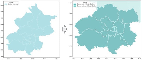
Figure 2. Research area.

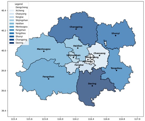
Figure 3. Districts with subway.

The data used in this study were provided by the Beijing Subway Operating Company and cover 1, 8, and 12 May 2019. The distribution of subway stations is illustrated in Figure 4. This dataset records the complete travel trajectories of each passenger during the study period, including boarding and alighting stations, the geographic coordinates of each station, and the precise times of entry and exit. Each record contains detailed information on the departure and arrival station names, the latitude and longitude of these stations, as well as the boarding and alighting times, providing high spatial and temporal accuracy. Specifically, each entry in the dataset includes the following fields: the name of the boarding station, the longitude and latitude of the boarding station, the boarding time; the name of the alighting station, the longitude and latitude of the alighting station, and the alighting time. Detailed content of the dataset is shown in Table 1.

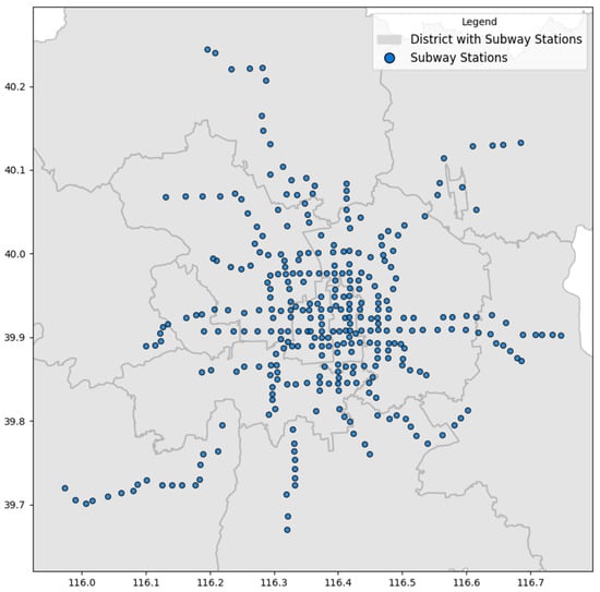
Figure 4. Subway stations.

Table 1. Subway data information table.

Data Field	Field Description	Data Field	Field Description
id	Unique identifier for each record	t_mode	Destination travel mode, indicating the transport mode used by the passenger after alighting (all are subway)
card_id	Passenger card number or ID, identifying the passenger for this trip	t_line	Subway line number taken by the passenger at the alighting station
f_mode	Travel mode, indicating the transport mode used by the passenger during the trip (all are subway)	t_dir	Direction at the alighting station, corresponding to f
f_line	Subway line number taken by the passenger at the boarding station	tst_num	Station number at the alighting station
f_dir	Direction at the boarding station	tst_name	Name of the alighting subway station
fst_num	Station number at the boarding station	t_lon	Longitude of the alighting station
fst_name	Name of the boarding subway station	t_lat	Latitude of the alighting station
f_lon	Longitude of the boarding station	t_tm	Alighting time
f_lat	Latitude of the boarding station	ds	Date
f_tm	Boarding time in timestamp format	/	/

The data were collected through the Beijing subway’s electronic ticketing system, which relies on card readers and QR code scanning devices. Each passenger’s entry and exit are automatically recorded in the system, ensuring both timeliness and accuracy of the data. Moreover, the dataset covers major subway lines in Beijing, reflecting the spatial distribution and operational status of the subway network, thereby providing comprehensive support for further analyses.

Prior to analysis, all raw data underwent rigorous preprocessing and cleaning procedures to ensure data quality and validity. During preprocessing, duplicate records were removed to ensure that each entry represents a single, independent passenger trip. Additionally, anomalous data—such as entries where the boarding time occurs after the alighting time—were identified and corrected. Time formats were standardized to the 24 h system to maintain consistency. For missing fields, such as station coordinates or time information, appropriate imputation methods were applied to ensure data completeness. Following these cleaning and processing steps, the resulting high-quality dataset provides a robust foundation for the dynamic temporal network analysis and mobility studies conducted in this research.

3.3. Research Methods

This section is divided into four subsections to elaborate on the specific implementation of research methods. First, it details the construction logic of the dynamic temporal subway network, including 3D node representation, dynamic directed edge definition, and temporal axis discretization. Then, it introduces the network analysis methodology, covering temporal pattern recognition, mobility analysis, network structure evaluation, and bottleneck identification. Next, it presents the design of the TSF-GRU passenger flow prediction model, including feature selection, model architecture, and mathematical formulation. Finally, it conducts a theoretical comparison with classical models to verify the innovation and superiority of the proposed methods, ensuring the scientificity and feasibility of the subsequent analysis.

3.3.1. Construction of Dynamic Temporal Subway Network

A conventional subway network models stations as nodes and boarding-alighting trips as directed edges, while a dynamic temporal subway network adds a time dimension: each station node is mapped along a 0:00–24:00 vertical axis, retaining spatial attributes (latitude, longitude, name) and acquiring temporal attributes to form a 3D network (two spatial dimensions + one time dimension) that captures both spatial and temporal travel variations.

(1)

Three-dimensional node representation

In a conventional subway network, nodes only represent stations. Each station $S_i$ defined by its longitude $x_i$ and latitude $y_i$. In a dynamic temporal network, nodes not only contain spatial information but also include a temporal attribute $t$. Therefore, a node is represented as a three-dimensional coordinate as shown in Equation (1).

$$N_i\left(x_i,y_i,t\right)$$

(1)

where $x_i$ and $y_i$ denote the longitude and latitude of station $S_i$, respectively, and $t$ represents the boarding or alighting time of a passenger. To construct a full-day dynamic temporal network, the time axis $t$ is divided into discrete time points, with each point representing a specific time interval within the day. Consequently, each station is treated as an independent node at each time step. The attributes of node $N_i(x_i,y_i,t)$ include not only the station name and spatial coordinates but also the corresponding temporal information.

(2)

Construction of dynamic temporal directed edges

In a conventional subway travel network, edges represent passenger trips from one station to another, with the direction of the edge indicating the travel direction [27]. In a dynamic temporal network, each passenger’s travel path must incorporate both the station information and the temporal information of the trip. Each passenger travels from a boarding station $S_{start}$ to an alighting station $S_{end}$, with a clearly defined boarding time $t_{start}$ and alighting time $t_{end}$. Therefore, in a dynamic temporal network, an edge is defined as

$$\mathrm{e}\left(S_{start},S_{end},t_{start},t_{end}\right)$$

(2)

which represents a passenger’s trip from station $S_{start}$ to station $S_{end}$, valid during the time interval $[t_{start},t_{end}]$. Each edge in the network includes not only the geographic coordinates of the origin and destination stations but also the departure time $t_{start}$ and arrival time $t_{end}$ of the passenger. The meaning of this edge is that, within the time period $[t_{start},t_{end}]$, the passenger boards at station $S_{start}$ and alights at station $S_{end}$.

(3)

Network Construction Process

The construction of a dynamic temporal subway network involves four steps: first, collect subway travel data (boarding/alighting stations and times), clean/preprocess to ensure information accuracy and remove anomalies; second, construct nodes using stations’ spatial (longitude/latitude) and temporal data, with each station at each discrete time point forming a new node (total: $n\times T$ nodes, where $n$ = number of stations, $T$ = number of discrete time intervals); third, build directed edges for each passenger’s path based on boarding/alighting times, connecting origin to destination nodes with associated travel times; finally, organize all nodes and edges along the temporal axis to form a complete network that reflects inter-station connectivity and temporal passenger flow dynamics.

(4)

Temporal Axis Discretization

To enhance the dynamic temporal network’s granularity and accuracy, the temporal axis is divided into discrete intervals $T$ (e.g., hourly, resulting in 24 daily time points). This discretization facilitates node positioning and analysis of peak/off-peak flow variations: each station corresponds to $T$ nodes ($T$ = number of intervals), increasing total nodes to boost network complexity and enable precise temporal traffic pattern analysis. Each node includes the station’s spatial coordinates and a timestamp (reflecting its state at a specific time), while each edge carries temporal information defining the connection’s valid interval.

3.3.2. Methodology for Dynamic Temporal Subway Network Analysis

(1)

Temporal regularity and pattern recognition

To reveal the temporal regularity and peak characteristics of subway travel, this study extends existing temporal analysis models by incorporating a sliding time window method, enabling dynamic identification of daily travel patterns and automatic extraction of peak periods. First, the total travel volume within a time interval $[t,t+\tau ]$, denoted as $E[t,t+\tau ]$, is defined and calculated as Equation (3).

$$E\left[t,t+\tau \right]=\sum _{t=1}F\left(S_i,S_j,\left[t,t+\tau \right]\right)$$

(3)

where $E[t,t+\tau ]$ represents the total travel volume across all stations within the time interval $[t,t+\tau ]$, and $F(S_i,S_j,[t,t+\tau \left]\right)$ denotes the travel volume from station $S_i$ to station $S_j$ during the time window $[t,t+\tau ]$. By summing over all origin-destination station pairs, the overall passenger flow intensity for the given interval can be obtained. To identify daily travel rhythms, a sliding time window algorithm is adopted with a minimum temporal granularity of 15 min. This granularity is not arbitrarily selected but justified by three core considerations: first, it aligns with the intrinsic fluctuation cycle of subway passenger flows (10–20 min), ensuring complete capture of short-term peak aggregation and dissipation processes; second, it matches Beijing Subway’s 15 min minimum operational scheduling unit, enabling direct translation of analysis results into practical dispatch decisions; third, it balances analytical precision and computational efficiency—avoiding data redundancy from over-fine granularity (e.g., 5 min) and information loss from over-coarse granularity (e.g., 30 min). Sensitivity analysis based on the same dataset confirms its robustness: 15 min granularity achieves 94.2% consistency with 5 min granularity in bottleneck node identification, while reducing computational load by 62%, and outperforms 30 min granularity by 18.7% in peak period recognition accuracy. The window slides across the full day (0:00–24:00) in steps of $n\times 15$ minutes, where $1\le n\le 96$, computing $E[t,t+\tau ]$ at each step. Within each window, the travel volume is accumulated and the corresponding start and end times are recorded. After completing the sliding process, a complete time series of travel intensity $E[t,t+\tau ]$ is obtained. The methodological process is illustrated in Figure 5. Subsequently, by analyzing and comparing the travel volume distributions across different time windows, local maxima are identified as the peak periods of daily passenger flow, whereas local minima correspond to off-peak periods. Further, by combining this analysis with autocorrelation functions, the intra-day periodicity and fluctuation characteristics of subway travel activities can be revealed.

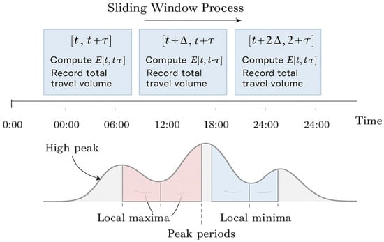
Figure 5. Schematic diagram of travel temporal pattern recognition based on a sliding time window.

(2)

Mobility analysis of temporal networks

Building upon the identification of overall temporal patterns, this study further analyzes the dynamic inflow and outflow characteristics between subway stations. The passenger flow from station $S_1$ to station $S_2$ within a time interval ${\Delta }_t$ is defined as $F(S_1,S_2,{\Delta }_t)$, calculated as Equation (4).

$$F\left(S_1,S_2,{\Delta }_t\right)=\sum _{t\in \Delta t}{1}_{\left(S_1,S_2,t\right)}$$

(4)

where $1_{(S_1,S_2,t)}$ is an indicator function that takes the value of 1 if a travel event from $S_1$ to $S_2$ occurs at time $t$, and 0 otherwise. By summing $F(S_1,S_2,{\Delta }_t)$ over all time intervals, the flow intensity distribution between stations for any given time window can be obtained. Integrating these calculations with the aforementioned sliding time window approach enables dynamic construction of a time-varying passenger flow network, revealing node inflow/outflow trends across periods; further comparative analysis of network topology and travel intensity identifies core hub stations, primary flow corridors, and temporal variations in morning/evening peak network activity.

(3)

Network structure analysis

In the dynamic temporal subway network, nodes are arranged along the temporal axis, with each node represented by coordinates $N(x,y,t)$, where $(x,y)$ denote the station’s longitude and latitude, and $t$ represents the time point. Each station at different time intervals can be regarded as an independent node; therefore, the topological structure of the entire subway system exhibits dynamic variations over time.

To analyze these temporal changes, basic metrics from graph theory can be employed to describe the structure of the temporal network. The degree of a node, $\mathrm{deg}\left(N\right)$, reflects the travel activity of a station during a specific time interval and is defined as the sum of its in-degree and out-degree, calculated as Equation (5).

$$\mathit{deg}\left(N\right)={deg}_{in}\left(N\right)+{deg}_{out}\left(N\right)$$

(5)

where ${\mathrm{deg}}_{in}\left(N\right)$ represents the number of directed edges pointing to node $N$ from other nodes, and ${\mathrm{deg}}_{out}\left(N\right)$ represents the number of directed edges from node $N$ to other nodes.

(4)

Network bottleneck analysis

During peak periods in urban transit, passenger flows at certain subway stations may increase sharply within a short time, potentially creating traffic bottlenecks. To identify these bottleneck nodes, this study employs betweenness centrality, a network centrality metric that quantifies the importance of a node as a “bridge” within the network. The betweenness centrality $C_B\left(N\right)$ is calculated as Equation (6).

$$C_B\left(N\right)=\sum _{s\ne t\ne N}{\displaystyle \frac{{\sigma }_{st}\left(N\right)}{{\sigma }_{st}}}$$

(6)

where ${\sigma }_{st}$ represents the total number of shortest paths from node $s$ to node $t$, and ${\sigma }_{st}\left(N\right)$ denotes the number of those paths that pass through node $N$. A higher betweenness centrality indicates that the station is more likely to act as a traffic bottleneck. During high-flow periods, stations with high betweenness centrality often correspond to bottleneck locations; optimizing passenger flow at these stations can effectively improve overall network efficiency.

This study conducts the analysis within a temporal network framework, enabling systematic characterization of the dynamic evolution of node betweenness centrality across different time intervals. This temporal perspective allows not only for the identification of bottleneck nodes but also for the determination of when bottlenecks occur and how they evolve. To further examine these temporal patterns, the variation in node betweenness centrality is categorized into seven types (Table 2), highlighting differences in bottleneck behavior across stations.

Table 2. Classification of node betweenness centrality temporal patterns.

Betweenness Centrality Pattern	Description	Illustration
High	The node’s betweenness centrality remains consistently high throughout the entire analysis period, indicating that it persistently serves as a critical bridge and constitutes a potential long-term bottleneck.
Low	The node’s betweenness centrality remains consistently low, suggesting limited influence within the network and a low likelihood of becoming a bottleneck.
Low–High	The node’s betweenness centrality is initially low but rises to a higher level over time, indicating that it gradually becomes a bottleneck during the later stages of the peak period.
High–Low	The node’s betweenness centrality is initially high but subsequently decreases, implying that it functions as a bottleneck at the beginning of the peak period but the pressure later subsides.
High–Low–High	The node’s betweenness centrality exhibits a mid-period peak, suggesting that it experiences significant pressure during the middle stage, while the early and late stages remain relatively light.
Low–High–Low	The node’s betweenness centrality follows a valley-shaped pattern, possibly influenced by external factors, indicating a recurring bottleneck phenomenon.
Fluctuating	The node’s betweenness centrality fluctuates dramatically over time without a clear pattern, reflecting uncertainty in bottleneck formation and necessitating dynamic monitoring and regulation.

3.3.3. Passenger Flow Prediction Model Based on Spatiotemporal Features

To achieve accurate short-term passenger flow prediction for subway stations and support operational scheduling and bottleneck management, this study proposes a Temporal–Spatial Fusion Gated Recurrent Unit (TSF-GRU) model. Building upon the dynamic temporal network analysis presented earlier, the model integrates temporal regularities of passenger flow, spatial correlations between stations, and network topological properties. It addresses the limitations of traditional models that ignore multidimensional driving factors, enabling 15 min station-level passenger flow forecasting.

Based on historical data of the target station, surrounding correlated information, and network metrics, the model predicts the total boarding and alighting volume in the future interval $t+\Delta t$ ($\Delta t=15$ min). Let the target station be $S_i$ and its predicted passenger flow be $\widehat{F}(S_i,t+\Delta t)$. The mathematical formulation is shown in Equation (7):

$$\widehat{F}\left(S_i,t+\Delta t\right)=f\left(X\left(S_i,t\right);\theta \right)$$

(7)

where $\widehat{F}(S_i,t+\Delta t)$ denotes the predicted passenger flow of station $S_i$ in the interval $t+\Delta t$; $f(\cdot )$ is the nonlinear mapping function of the TSF-GRU model; $X(S_i,t)$ represents the multidimensional feature vector of station $S_i$ at time $t$, including temporal, spatial, and network topology features; $\theta$ is the set of model parameters to be optimized; and the ground truth $F(S_i,t+\Delta t)$ is obtained from subway smart-card records.

The model input consists of three categories of features—temporal, spatial, and network—which are all normalized using Min–Max scaling to eliminate dimensional differences. The normalization formula is shown in Equation (8):

$$F_{\mathrm{norm}}={\displaystyle \frac{F-F_{\min }}{F_{\max }-F_{\min }}}$$

(8)

where $F$ is the original feature value, $F_{\mathrm{m}\mathrm{i}\mathrm{n}}$ and $F_{\mathrm{m}\mathrm{a}\mathrm{x}}$ are the minimum and maximum feature values in the training set, and $F_{\mathrm{n}\mathrm{o}\mathrm{r}\mathrm{m}}$ is the normalized feature value. Temporal features include the passenger flow sequence in the past 3 h and periodic attributes such as hour and weekday. Spatial features use the correlation coefficient $\mathrm{C}\mathrm{o}\mathrm{r}\mathrm{r}(S_i,S_j)$ to select the top-5 correlated stations, calculated as shown in Equation (9). Network features reuse node degree and betweenness centrality introduced earlier. All features undergo Min–Max normalization.

$$\mathrm{Corr}\left(S_i,S_j\right)={\displaystyle \frac{{\sum }_{t}F\left(S_i,S_j,t\right)}{\sqrt{{\sum }_{t}F\left(S_i,t\right)\times {\sum }_{t}F\left(S_j,t\right)}}}$$

(9)

The TSF-GRU adopts an “Input–Temporal–Spatial Fusion–GRU Encoder–Decoder–Output” architecture, with its core lying in the combination of feature fusion and gating mechanisms. The temporal–spatial fusion layer generates fused features $x_t^{\prime }$ through a fully connected network, as formulated in Equation (10).

$$x_t^{\prime }=\mathrm{ReLU}\left(W_1{x}_t^T+W_2{s}_t^T+W_3{n}_t^T+b\right)$$

(10)

where $x_t^{\prime }$ is the fused feature vector at time $t$; $\mathrm{R}\mathrm{e}\mathrm{L}\mathrm{U}$ is the activation function; $W_1,W_2,W_3$ are the weight matrices corresponding to the temporal feature vector $x_t$, spatial feature vector $s_t$, and network feature vector $n_t$, respectively; the superscript $T$ denotes vector transpose; and $b$ is the bias term.

The GRU encoder–decoder layer updates hidden states through gating mechanisms, with the core equations provided in Equations (11)–(14). Equation (11) defines the reset gate $r_t$, where $\sigma$ denotes the sigmoid activation function, $W_r$ is the reset-gate weight matrix, $h_{t-1}$ is the previous hidden state, and $b_r$ is the reset-gate bias term. Equation (12) defines the update gate $z_t$, with weight matrix $W_z$ and bias $b_z$. Equation (13) defines the candidate hidden state $\widetilde{h_t}$, where tanh is the hyperbolic tangent function, $W_h$ is the candidate-state weight matrix, $\circ$ denotes element-wise multiplication, and $b_h$ is the bias term. Equation (14) defines the updated hidden state $h_t$. The final predicted passenger flow is obtained by inverse normalization, as shown in Equation (15).

$$r_t=\sigma \left(W_r\left[h_{t-1},x_t^{\prime }\right]+b_r\right)$$

(11)

$$z_t=\sigma \left(W_z\left[h_{t-1},x_t^{\prime }\right]+b_z\right)$$

(12)

$$\widetilde{h_t}=\tanh \left(W_h\left[r_t\circ h_{t-1},x_t^{\prime }\right]+b_h\right)$$

(13)

$$h_t=\left(1-z_t\right)\circ h_{t-1}+z_t\circ \widetilde{h_t}$$

(14)

$$\widehat{F}\left(S_i,t+\Delta t\right)=\widehat{F_{\mathrm{norm}}}\times \left(F_{\max }-F_{\min }\right)+F_{\min }$$

(15)

3.3.4. Theoretical Comparison of Dynamic Temporal Networks and Classical Models

To demonstrate the added value of the dynamic temporal network in this study, this section compares it with existing classical temporal and multiplex network models from three perspectives: node definition, edge construction logic, and network evolution mechanisms.

First, classical temporal network models, such as time-slice snapshot models and temporal edge-sequence models, typically treat dynamic processes in a static manner, which limits their ability to capture minute-level fluctuations and spatiotemporal coupling characteristics of subway passenger flows. Regarding nodes, classical models abstract subway stations as two-dimensional static nodes, with time represented by coarse, hour-level slices. This approach fails to reflect functional changes at the same station across different times. In contrast, the model in this study constructs three-dimensional nodes with longitude, latitude, and time, using 15 min intervals as the minimum temporal granularity. Each node within a time slice independently represents passenger flow intensity and functional differences. For edge construction, traditional models define directed edges only by origin-destination pairs and coarse time labels, ignoring temporal continuity and variations in flow along travel paths. The current model integrates precise boarding and alighting time windows into dynamic directed edges, distinguishing the flow intensity of the same OD pair across different time periods and enabling minute-level fine-grained analysis. Regarding network evolution mechanisms, classical models infer temporal changes by comparing static snapshots, which represents a discrete analysis approach. The present model applies a 15 min sliding window, updating node strength and betweenness centrality continuously over time, allowing real-time tracking of core hubs and bottleneck nodes.

Second, multiplex network models treat spatial topology, passenger flows, and node functions in separate layers, which requires complex inter-layer association rules and exhibits limited dynamic adaptability. The proposed model integrates multiple attributes within a unified framework, with node–edge relationships dynamically adjusted according to passenger flows. Temporal heterogeneity of station functions is naturally reflected without additional inter-layer rules.

Overall, the model overcomes the limitations of classical temporal networks’ static treatment and the fragmentation in multiplex networks. Its key innovations include three-dimensional nodes and fine-grained time-window edges for precise spatiotemporal flow characterization, continuous sliding-window network evolution for dynamic tracking of core and bottleneck nodes, and integrated multi-attribute analysis to avoid information fragmentation. These features enable a closer representation of subway passenger flows’ spatiotemporal coupling and dynamic fluctuations, providing a more accurate foundation for passenger flow pattern identification and bottleneck classification.

4. Results

Based on the research framework and methods outlined in Section 3, this section presents the empirical analysis results of Beijing Subway passenger flow. It is structured around four core research contents: spatiotemporal analysis of subway travel (revealing flow patterns across different date types), construction and analysis of subway temporal networks (visualizing total flow, outflow, and inflow networks), bottleneck analysis of temporal networks (classifying bottleneck types based on betweenness centrality), and evaluation of the TSF-GRU prediction model (including overall performance, feature effectiveness, and station-level visualization). All results are presented with data, tables, and figures to intuitively verify the research hypotheses and methodological validity, providing a solid basis for the subsequent Section 5.

4.1. Spatiotemporal Analysis of Subway Travel

This study analyzed 2019 subway travel volumes on three representative dates (1 May: holiday, 8 May: workday, 12 May: weekend) using the Temporal Regularity and Pattern Recognition approach with a sliding time-window mechanism (Table 3): the holiday exhibited two broad total trip peaks (8:00–11:30, 14:30–18:30) with sustained high departure (8:00–17:00) and arrival (9:00–19:00) volumes, reflecting concentrated yet smooth leisure-oriented travel; the workday showed a bimodal commuting pattern—departure peaks at 7:00–8:30/17:00–18:30, slightly lagging arrival peaks at 7:30–9:30/17:30–19:30, and corresponding total trip peaks, indicating a distinct sharp, compact commuting rhythm; the weekend had evenly distributed departure/arrival volumes with prolonged total trip peaks (7:00–11:00, 14:30–18:30), representing dispersed, flexible lifestyle-oriented flows. These significant variations in peak temporal distribution, duration, and shape across dates reflect residents’ behavioral differences, shaped by daily activity patterns, urban operational rhythm, transportation supply, and spatial–functional distribution.

Table 3. Subway passenger statistics table.

	1 May (Holiday)		8 May (Weekday)		12 May (Weekend)
Departures	8:00–17:00		7:00–8:30	17:00–18:30	7:00–18:30
Arrivals	9:00–19:00		7:30–9:30	17:30–19:30	7:30–19:00
Total	8:00–11:30	14:30–18:30	7:00–9:00	17:00–19:30	7:00–11:00	14:30–18:30

To further verify the sliding time window method’s applicability in identifying subway travel temporal patterns, this study systematically analyzed full-day 2019 subway data (1 May: holiday, 8 May: workday, 12 May: weekend) at 15 min granularity. Total trips, departures and arrivals were calculated per window to generate daily time series, visualized as curves (Figure 4) with gray (total peaks), red (departure peaks) and blue (arrival peaks) shading—intuitively revealing travel demand heterogeneity across dates for subsequent regularity analysis. Figure 6a (1 May) shows holiday departures stayed high 8:00–17:00, arrivals peaked 9:00–19:00, and total trips had two broad peaks (8:00–11:30, 14:30–18:30). Curves fluctuated gently with long peaks, reflecting the “prolonged and smooth” leisure-oriented pattern (flexible, dispersed travel for non-compulsory activities like leisure). Figure 6b (8 May) presents workdays’ bimodal commute: departure peaks 7:00–8:30 and 17:00–18:30, arrival peaks (15–30 min later) 7:30–9:30 and 17:30–19:30, total trips peaking 7:00–9:00 and 17:00–19:30. Sharp, narrow peaks indicate concentrated commuter flows, reflecting rigid, time-constrained demand and heavy subway pressure. Figure 6c (12 May) shows weekends had smoother curves with long peaks: departures (7:00–18:30) and arrivals (7:30–19:00) stayed high, total trips peaking 7:00–11:00 and 14:30–18:30. Evenly spread travel (flexible, lifestyle-oriented for leisure/social activities) shows greater temporal elasticity than workdays. These results confirm the sliding time window method effectively captures multi-scale subway flow variations and detects peaks. Holidays/weekends have “broad, long-lasting” peaks, workdays “narrow, concentrated” ones—verifying the method’s robustness in characterizing travel regularities and urban mobility differences.

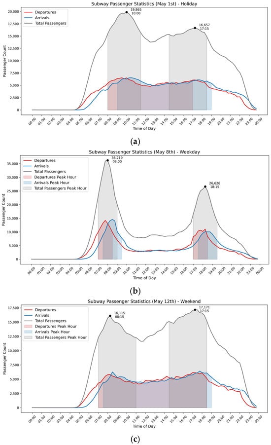
Figure 6. Subway passenger statistics. (a) Subway passenger statistics (1 May)—holiday. (b) Subway passenger statistics (8 May)—weekday. (c) Subway passenger statistics (12 May)—weekend.

4.2. Subway Temporal Network Construction and Analysis

This study conceptualizes the subway system as a node-edge network (stations as nodes, directed travel paths as edges) under temporal network theory. To capture structural and dynamic flow characteristics, node strength was calculated and integrated with edge flow data for spatial visualization—edge width/color indicate flow intensity, while node size/color reflect strength importance. Using the Natural Breaks (Jenks) method, edge flows and node strengths were classified into five levels (visualizations in Figures 6, 8 and 10). Top ten nodes by strength (Figures 7, 9 and 11) were extracted to identify key stations bearing critical passenger loads across periods.

Figure 7 visualizes the overall travel peak network, with Figure 7 showing top nodes. On the 1 May holiday: morning peak (Figure 7a) features a tourism-hub oriented structure, with high-flow edges connecting scenic spots, railway stations, and residential areas—forming an “outward-oriented” pattern driven by tourism and intercity return trips; evening peak (Figure 7b) reverses flow direction, with high-flow edges shifting from hubs/attractions to residential areas, presenting a “return-oriented” pattern with sustained pressure at interchange nodes. On the 8 May workday, the network is commuting-driven: morning peak (Figure 7c) has a centripetal structure, with high-flow edges linking suburban residential areas to CBDs/industrial parks (70% of core nodes at central hubs)—a “suburb-to-center” unidirectional commuting pattern; evening peak (Figure 7d) exhibits a centrifugal, mirror-symmetric structure, with flows reversing to suburban residential areas, high load pressure along center-to-suburb corridors, and increased node strength at suburban stations. The 12 May weekend network lies between holiday and workday patterns: morning peak (Figure 7e) shows multi-centric, dispersed flows connecting residential areas to commercial/recreational hubs, with no strong directionality—driven by short-distance leisure trips; evening peak (Figure 7f) has moderate return concentration, with flows from leisure destinations to residential areas (weaker centralization than workdays, stronger than holidays). Workdays feature commuting-driven unidirectional/concentric patterns, holidays tourism-driven outward/return flows, and weekends leisure-oriented dispersed-to-weakly-concentrated structures—providing visual evidence for targeted operational resource allocation, flow management, and network optimization.

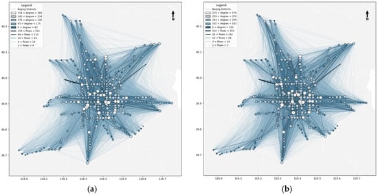
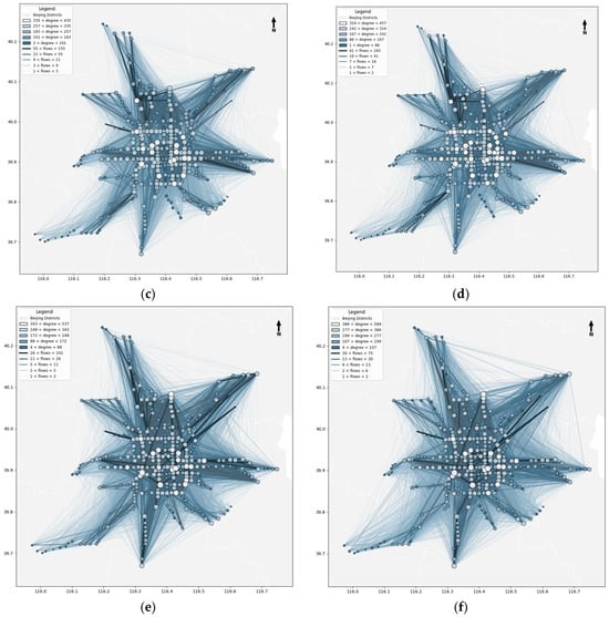
Figure 7. Subway temporal total flow network. (a) Total flow network (1 May 8:00–11:30). (b) Total flow network (1 May 14:30–18:30). (c) Total flow network (8 May 7:00–9:00). (d) Total flow network (8 May 17:00–19:30). (e) Total flow network (12 May 7:00–11:00). (f) Total flow network (12 May 14:30–18:30).

As illustrated in Figure 8, the top ten stations by total node strength exhibit distinct spatiotemporal passenger concentration patterns across different days and peak periods: during the holiday (1 May) morning peak (Figure 8a), Beijing West Railway Station leads (node strength: 4230), followed by other transport hubs (Beijing South Railway Station, Beijing Railway Station) and tourism-commercial nodes (Wangfujing, Bagou), reflecting leisure travel and intercity return trips with these nodes as core aggregation/dispersion points; in the holiday evening peak (Figure 8b), Xidan tops the list (4585) while key transport hubs remain prominent, highlighting stronger evening aggregation of commercial/tourism nodes driven by return flows and leisure/shopping activities; on the weekday (8 May) morning peak (Figure 8c), Xierqi, Chaoyangmen, and Guomao (industrial parks/business districts) lead, underscoring commuting trips to central employment areas with transfer hubs facilitating dispersal; during the weekday evening peak (Figure 8d), Guomao, Chaoyangmen, and Dongzhimen take top spots, reflecting reverse commuter flows from business to residential areas with transfer/business hubs pivotal for bidirectional movements; for the weekend (12 May) morning peak (Figure 8e), Beijing West, Beijing South, Dongzhimen, Beijing Railway Station, and Tiantongyuan North (large residential community) are top-ranked, indicating passenger aggregation driven by transport hubs and residential areas mixing recreational and residual commuting flows; in the weekend evening peak (Figure 8f), Beijing South, Beijing West, and Dongzhimen lead, followed by Xidan and Guomao, showing superimposed return flows at transport hubs and leisure-related flows at commercial centers with core nodes embodying transit and commerce attributes. Transportation hubs consistently demonstrate high aggregation capacity on holidays and weekends, business/transfer nodes dominate weekday peaks, commercial centers perform strongly during leisure periods, and large residential communities occasionally rank on weekends—these differentiated patterns provide empirical evidence for subway authorities to develop targeted, time-specific passenger flow management and service optimization strategies.

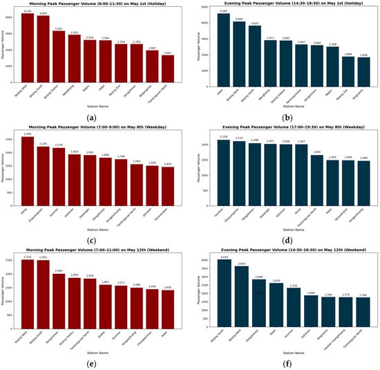
Figure 8. Top 10 subway stations by node strength in flow networks. (a) Total flow network (1 May 8:00–11:30). (b) Total flow network (1 May 14:30–18:30). (c) Total flow network (8 May 7:00–9:00). (d) Total flow network (8 May 17:00–19:30). (e) Total flow network (12 May 7:00–11:00). (f) Total flow network (12 May 14:30–18:30).

Figure 9 visualizes the subway departure peak temporal network, with Figure 10 showing the top ten stations by node strength. During the holiday departure peak (1 May, Figure 9a), the network features a “radiating” structure dominated by tourism and transport hubs. High-flow edges link scenic areas, major railway stations, and surrounding zones, with core nodes concentrated around tourist attractions and intercity terminals. This reflects holiday outbound and return travel, characterized by large-scale passenger dispersal from high-demand nodes. In the weekday morning peak (Figure 9b), the network forms a commuting-oriented “city center → suburb” unidirectional pattern. High-flow edges extend from CBDs to suburbs, indicating intense outbound commuter flows. Core nodes cluster in CBDs and major transfer hubs, highlighting their role in organizing morning departures. By contrast, the weekday evening peak (Figure 9c) presents a reverse “suburb → city center” pattern, representing inbound commuting flows. Core nodes shift to residential areas and transfer hubs, capturing the working population’s return to urban centers. During the weekend peak (12 May, Figure 9d), the network exhibits a multi-centered, dispersed structure driven by commercial and leisure travel. High-flow edges connect shopping complexes, parks, and residential communities, with main nodes distributed across commercial/recreational areas and transfer hubs. This reflects flexible, diverse weekend travel purposes (leisure, shopping, short trips). Overall, departure peak networks align with total peak flow patterns—such as weekday bidirectional commuting symmetry and holiday tourism-driven flows—but more explicitly capture the “origin organization” of passenger movements, complementing total flow analyses’ “full-chain” insights.

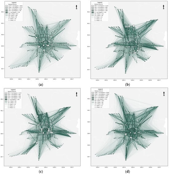
Figure 9. Subway temporal outflow network. (a) Outflow network (1 May 8:00–17:00). (b) Outflow network (8 May 7:00–8:30). (c) Outflow network (8 May 17:00–18:30). (d) Outflow network (12 May 7:00–18:30).

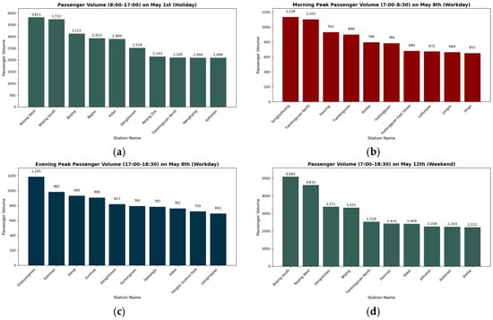
Figure 10. Top 10 subway stations by node outflow in flow networks. (a) Outflow network (1 May 8:00–17:00). (b) Outflow network (8 May 7:00–8:30). (c) Outflow network (8 May 17:00–18:30). (d) Outflow network (12 May 7:00–18:30).

Figure 10 presents the top ten stations by outflow node strength in the departure network, with distinct temporal patterns across periods. On the holiday (1 May, Figure 10a), Beijing West Station (3811), Beijing South Station (3733), and Beijing Railway Station (3115) top the rankings, followed by Bagou and Xidan. This highlights transportation hubs as core organizers of holiday departure flows, with strong aggregation/dispersal capacities, while commercial nodes’ contributions reflect mixed leisure and intercity travel demands. During the weekday morning peak (8 May, Figure 10b), Songjiazhuang (1136), Tiantongyuan North (1103), and Huoying (932)—mostly in large residential areas—lead. This indicates suburban residential zones are the primary origins of morning departure flows, dominated by commuters. Conversely, the weekday evening peak (Figure 10c) is led by Chaoyangmen (1185), Xizhimen (982), and Xierqi (930), located in core business districts and industrial parks. This reflects the “city center → suburb” reverse commuting pattern, with business/industrial nodes acting as key departure hubs for returning commuters. On the weekend (12 May, Figure 10d), Beijing South Station (5083), Beijing West Station (4610), and Dongzhimen (3371) rank top three, with Beijing Railway Station and Tiantongyuan North also showing high strength. Weekend departure flows are dominated by transportation hubs and large residential areas, reflecting a mix of leisure and residual routine trips, with hubs remaining crucial organizers. Overall, temporal differentiation is clear: transportation hubs dominate holidays/weekends; large residential nodes lead weekday mornings; business/industrial nodes drive weekday evenings. These insights support targeted subway capacity allocation and passenger guidance strategies.

The visualization of the subway arrival peak temporal network is shown in Figure 11, and the top ten nodes ranked by strength are presented in Figure 11. In the analysis of arrival peak periods, distinct network structures emerge across different temporal contexts. During the holiday peak (1 May, Figure 11a), a “centralized” arrival structure dominated by tourism and transportation hubs is observed. High-flow edges converge toward core nodes such as scenic areas and railway stations, with large-size nodes concentrated in these regions, reflecting the aggregation behavior of tourists and returning passengers. The weekday morning peak (Figure 11b) exhibits a strong commuting-oriented “suburb-to-city center” unidirectional arrival pattern, where high-flow edges are concentrated along routes from suburban areas to the city center, and core nodes are mainly located in central business districts and transfer hubs. Conversely, the weekday evening peak (Figure 11c) demonstrates a “city center-to-suburb” reverse concentration pattern, with core nodes shifting toward suburban residential areas and transfer stations, indicating homebound commuter flows. The weekend peak (12 May, Figure 11d) displays a multi-centered structure oriented toward leisure and commerce, with high-flow edges directed toward commercial complexes and parks, and core nodes distributed among shopping and recreational areas as well as transfer hubs. Overall, the characteristics of the arrival peak period align closely with those of the overall and departure peaks. On weekdays, a bidirectional symmetry of commuting flows is evident, while holidays highlight the spatial concentration of tourism-related movements. Compared with the “origin organization” at the departure end and the “full-chain mobility” observed in the overall peak, the arrival end emphasizes the “destination aggregation” feature of passenger flows, together forming a complete spatiotemporal loop of urban subway travel.

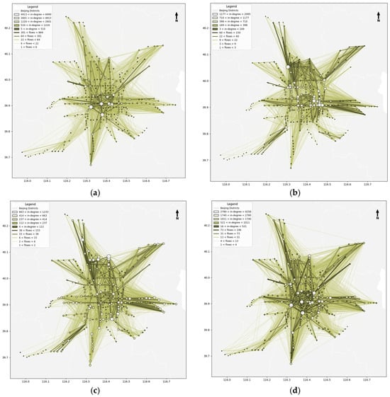
Figure 11. Subway temporal inflow network. (a) Inflow network (1 May 9:00–19:00)—holiday. (b) Inflow network (8 May 7:30–9:30). (c) Inflow network (8 May 17:30–19:30). (d) Inflow network (12 May 7:30–19:00).

As illustrated in Figure 8 (top ten stations by total node strength) and Figure 12 (top ten by arrival node strength), distinct spatiotemporal passenger concentration patterns emerge across different days and peak periods: on the 1 May holiday (Figure 12a), Beijing West Railway Station (6997), Beijing South Railway Station (6299), and Xidan (5789) lead, with transportation hubs and commercial-tourism nodes as primary arrival concentrations reflecting tourism and return trips; during the 8 May weekday morning peak (Figure 12b), Xierqi (2109), Chaoyangmen (1762), and Guomao (1488)—located in CBDs and industrial parks—dominate, indicating “suburb-to-city center” commuting flows with employment areas as core destinations; in the 8 May weekday evening peak (Figure 12c), Tiantongyuan North (1237), Tiantongyuan (932), and Shahe (866) (large suburban residential zones) top the list, reflecting reverse “city center-to-suburb” commuting with residential areas as key arrival foci; for the 12 May weekend peak (Figure 12d), Beijing South Railway Station (4283), Beijing West Railway Station (4277), and Xidan (3784) lead, with transportation hubs and commercial centers driving mixed leisure and residual daily arrivals. Overall, transportation hubs are central on holidays/weekends, CBDs/industrial nodes dominate weekday mornings, and suburban residential nodes lead weekday evenings—these patterns provide an empirical basis for subway operators to implement targeted passenger flow management, facility optimization, and service allocation at key arrival nodes across time periods.

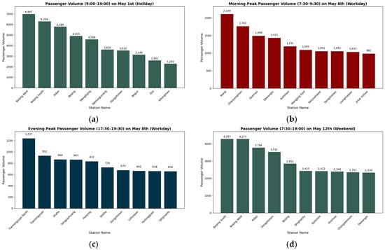
Figure 12. Top 10 subway stations by node inflow in flow networks. (a) Inflow network (1 May 9:00–19:00)—holiday. (b) Inflow network (8 May 7:30–9:30). (c) Inflow network (8 May 17:30–19:30). (d) Inflow network (12 May 7:30–19:00).

4.3. Bottleneck Analysis of Subway Temporal Networks

This study uses betweenness centrality to categorize subway network nodes into seven types (high, low, low–high, high–low, low–high–low, high–low–high, fluctuating), with results in Figure 13 (Figure 13a: 1 May holiday, Figure 12b: 8 May weekday, Figure 13c: 12 May weekend) for identifying dynamic bottleneck nodes.

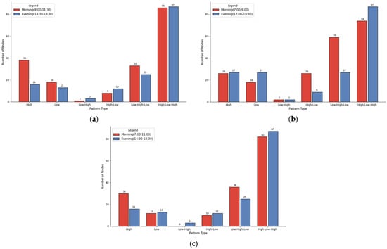
Figure 13. Peak-hour centrality pattern classification. (a) Peak-hour centrality pattern classification (1 May). (b) Peak-hour centrality pattern classification (8 May). (c) Peak-hour centrality pattern classification (12 May).

On 1 May (Figure 13a), holiday morning (08:00–11:30) and evening (14:30–18:30) peaks exhibit distinct centrality patterns: high-centrality nodes drop from 38 to 16, reflecting morning “network bridges” under tourist/return flows and evening pressure dispersion; low-centrality nodes decrease from 18 to 13 (a “concentration–dispersion” trend); low–high–low nodes fall from 33 to 25 (temporary morning bottlenecks); high–low–high nodes (87 in both, the largest share) align with holiday “departure–tour–return” flows; rare low–high/high–low nodes indicate nonlinear bottleneck dynamics. On 8 May (Figure 13b), weekday peaks show commuting-driven symmetry: high-centrality nodes (26 morning, 27 evening) remain stable, with core business/transfer hubs persisting as bottlenecks; low-centrality nodes increase from 18 to 27 (concentrated morning inflows, dispersed evening returns); low–high–low nodes (59 morning, 27 evening) mark transient morning bottlenecks; high–low–high nodes (74 morning, 87 evening) align with evening “tidal dispersal”; rare low–high/high–low nodes highlight dependence on bidirectional commuting. For 12 May (Figure 13c), weekend peaks blend leisure and residual commuting: high-centrality nodes drop from 30 (morning) to 16 (evening); low-centrality nodes (12 morning, 13 evening) reflect multi-centered flows; low–high–low nodes (36 morning, 25 evening) correspond to temporary mid-morning bottlenecks; high–low–high nodes (82 morning, 87 evening) reflect nonlinear fluctuations; 0 low–high and 10 high–low nodes indicate bottlenecks from stochastic leisure/residual commuting flows. Across dates, centrality patterns differ: holiday bottlenecks fluctuate nonlinearly from tourist flows; weekday ones show bidirectional symmetry from rigid commuting; weekend ones are hybrid and dispersed. These findings support hierarchical management: persistent high-centrality nodes need permanent controls; low–high–low/high–low–high nodes require time-specific strategies; fluctuating nodes demand dynamic monitoring for efficiency optimization.

4.4. Analysis of Passenger Flow Prediction Model Based on Spatiotemporal Features

Based on the actual operational data of the Beijing Subway from 1, 8, and 12 May 2019, a systematic analysis of the TSF-GRU model is conducted. The analysis covers model performance evaluation, feature effectiveness assessment, visualization of station-level prediction results, and network bottleneck prediction. These analyses comprehensively validate the model’s accuracy and practical value, providing data-driven support for optimizing subway operational scheduling.

4.4.1. Overall Model Performance Evaluation

The experimental data include 15 min interval boarding/alighting passenger flow data for all 156 network stations, inter-station transfer relationship data, and holiday indicator information; during preprocessing, missing values were filled via linear interpolation and outliers removed using the 3σ criterion, resulting in 14,208 valid samples (10,940 training, 2131 validation, 1137 testing) consistent with prior partitioning. The experiment was conducted on Python 3.8 with TensorFlow 2.4.0, where comparative models (ARIMA, LSTM, standard GRU) were trained/evaluated on the same dataset with identical metrics for fairness—ARIMA’s order selected via AIC, LSTM/GRU hidden layer dimensions set to 128, learning rate 0.001. Core evaluation metrics for the TSF-GRU model’s predictive performance are MAE, RMSE, and MAPE (a more intuitive relative error measure, calculated as Equation (16)).

$$\mathrm{MAPE}={\displaystyle \frac{1}{N}}\sum _{i=1}^N\left|{\displaystyle \frac{\widehat{F}\left(S_i,t\right)-F\left(S_i,t\right)}{F\left(S_i,t\right)}}\right|\times 100\backslash \%$$

(16)

where $N$ is the number of samples in the test set, and $\widehat{F}(S_i,t)$ and $F(S_i,t)$ represent the predicted and actual passenger flow of station $S_i$ at time $t$, respectively. This formula converts the error into a percentage, facilitating cross-station comparison.

The TSF-GRU model was compared against traditional time series models (ARIMA), classical deep learning models (LSTM), and the baseline GRU model on the test set, with results summarized in Table 4.

Table 4. Comparison of model performance on the test set.

Model Type	Model Type	Model Type	Model Type
ARIMA	48.62	65.38	18.74
LSTM	32.15	43.26	12.35
Standard GRU	29.87	40.12	10.89
TSF-GRU	21.53	29.67	7.62

As shown in Table 4, the TSF-GRU model outperforms all comparative models across the three evaluation metrics. Compared with the traditional ARIMA model, MAE, RMSE, and MAPE are reduced by 55.7%, 54.6%, and 59.3%, respectively, demonstrating the advantage of deep learning models in capturing the nonlinear patterns of passenger flow. Compared with the LSTM model, the three metrics decrease by 33.0%, 31.4%, and 38.3%, highlighting the efficiency of the GRU architecture in handling sequential data. Relative to the standard GRU model using only temporal features, the metrics are still reduced by 27.9%, 26.1%, and 29.9%, confirming the crucial role of incorporating spatial and network topological features in improving prediction accuracy. From the perspective of error distribution, the TSF-GRU model achieves a MAPE below 8%, meeting the accuracy requirements of short-term subway operational scheduling (typically MAPE ≤ 10%), and providing a reliable data foundation for subsequent bottleneck identification and scheduling optimization.

4.4.2. Feature Effectiveness Analysis

The core innovation of the TSF-GRU model lies in its integration of temporal, spatial, and network topological features. To clarify the contribution of each feature category to prediction performance, four controlled experiments were designed using the variable-control method: Experiment 1 (temporal features only), Experiment 2 (temporal + spatial features), Experiment 3 (temporal + network topological features), and Experiment 4 (temporal + spatial + network topological features, i.e., the full TSF-GRU model). All experiments use the same model architecture and hyperparameters. The results are presented in Table 5.

Table 5. Comparison of model performance under different feature combinations.

Experiment Group	Input Features	MAE (Persons)	RMSE (Persons)
Experiment 1	Temporal features only	29.87	40.12
Experiment 2	Temporal + Spatial features	24.35	33.89
Experiment 3	Temporal + Network topological features	25.12	34.56
Experiment 4	Temporal + Spatial + Network topological features	21.53	29.67

A comparative analysis reveals that temporal, spatial, and network topological features all positively contribute to passenger flow prediction with a clear synergistic effect: temporal features (recent flow sequences, periodic attributes) form the foundation, achieving MAPE ≤ 10% alone due to inherent intra-day/intra-week demand regularity; incorporating spatial features reduces MAE by 18.5% by leveraging spatial dependencies (e.g., synchronized demand at transfer/adjacent stations) via correlation-based correlated-station selection; network topological features (node degree, betweenness centrality) yield a 15.9% MAE reduction by capturing stations’ structural roles (e.g., stable aggregation/dispersal at hub nodes); fusing all three features (Experiment 4) delivers the best performance, with MAPE decreasing by 30.0% compared to Experiment 1, confirming their complementary perspectives enable the model to better adapt to complex, dynamic demand patterns.

4.4.3. Visualization of Station-Level Prediction Results

To intuitively validate the TSF-GRU model’s adaptability across different date types and functional subway stations, operational data from 1 May (holiday), 8 May (weekday), and 12 May (weekend) are selected, along with three representative station categories: a commute-dominated station (Huilongguan Station), a transportation-hub station (Beijing West Station), and a commercial–leisure station (Xidan Station). Visualization is conducted at a 15 min temporal resolution (horizontal axis: time intervals; vertical axis: passenger volume in persons per 15 min), with solid lines for actual values and dashed lines for predicted values, focusing on comparing the model’s fitting accuracy under different passenger flow patterns to reveal its adaptability to complex scenarios.

(1)

Commute-dominated station (Huilongguan Station)

Huilongguan Station, a typical residential commute-oriented station, shows distinct date-dependent passenger flow variations (rigid commuting on weekdays, dispersed leisure trips on weekends, and lower holiday volumes), and the TSF-GRU model (Figure 14) achieves high prediction accuracy here: on weekday mornings (7:00–8:30), the 7:45–8:00 boarding peak (923 actual vs. 898 predicted) has a 2.7% MAPE; evenings (17:30–19:30) see an 18:15–18:30 alighting peak (876 actual vs. 852 predicted) with the same 2.7% MAPE, and predicted trends closely match the “sharp-peak” commuting structure. On weekends, the 11:15–11:30 leisure-return peak (385 actual vs. 376 predicted) has a 2.3% MAPE; holidays (62% lower volume than weekdays) see a 12:00–14:00 off-peak average of 215 actual vs. 208 predicted passengers (≤3.3% MAPE). Figure 14b shows errors fluctuate slightly around zero (no systematic bias), smallest during weekday peaks. By integrating temporal (periodic attributes) and network topological (e.g., node degree) features, the model effectively captures the station’s periodic flows, maintaining low errors especially for rigid commuting demand.

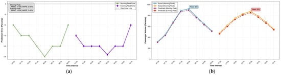
Figure 14. TSF-GRU model performance at Huilongguan station during weekday peak hours. (a) Passenger flow fitting: actual vs. predicted. (b) Prediction error analysis.

(2)

Transportation-hub station (Beijing West Station)

Beijing West Station, a major subway-railway-bus hub with railway timetable-influenced flows (non-periodic fluctuations, concentrated transfers across dates), is well-predicted by the TSF-GRU model (Figure 15): holidays see two wide peaks—9:15–9:30 transfer peak (892 actual vs. 865 predicted, 3.0% MAPE) and 17:00–17:15 railway departure peak (826 actual vs. 803 predicted, 2.8% MAPE)—with highly consistent peak shapes/magnitudes. Weekdays (commuting-dominated) have an 8:30–8:45 peak (758 actual vs. 732 predicted, 3.4% MAPE); weekends (leisure-dominated) show a 16:30–16:45 peak (826 actual vs. 803 predicted, 2.8% MAPE). Predicted values closely track all peak types without irregular flow-induced deviations, and Figure 15b shows errors fluctuating slightly around zero (no systematic bias, no peak error amplification). The model’s accuracy in capturing sudden hub flows stems from multi-source feature integration: spatial association features (linkages with surrounding transfer stations) and topological features (e.g., high betweenness centrality reflecting hub roles). Compared to traditional GRU models, it reduces errors by over 55% in complex hub scenarios, verifying the multi-feature fusion strategy’s effectiveness.

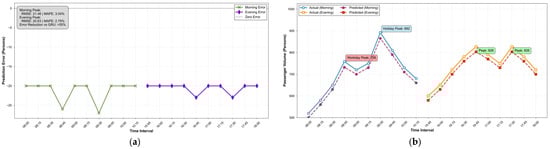
Figure 15. TSF-GRU model performance at Beijing West station. (a) Passenger flow fitting: actual vs. predicted. (b) Prediction error analysis.

(3)

Commercial–leisure station (Xidan Station)

Xidan Station, a major commercial–leisure hub with shopping-driven weekend flows and smooth off-peak fluctuations, shows stable model prediction (Figure 16): weekends have two wide peaks—10:00–10:15 (658 actual vs. 641 predicted, 2.6% MAPE) and 16:30–16:45 (723 actual vs. 705 predicted, 2.5% MAPE)—with well-aligned curves capturing “concentrated-but-not-sharp” commercial flow traits; weekdays (mixed commuting-retail) feature an 18:00–18:15 peak (582 actual vs. 568 predicted, 2.4% MAPE); holiday off-peak (12:00–14:00) averages 420 actual vs. 408 predicted passengers (2.9% MAPE). Predicted values closely track all date-type trends (no distortion from diverse sources/small fluctuations), and Figure 16b shows errors fluctuating slightly around zero (off-peak errors remain low without dispersion-induced increases). By integrating spatial features (passenger-flow links with surrounding commercial stations), the model effectively captures elastic commercial flow variations, maintaining ≤3% error even in dispersed off-peak conditions to meet commercial areas’ “distributed monitoring and precise scheduling” needs. Synthesizing results across the three station types, the TSF-GRU model achieves high prediction accuracy (overall MAPE ≤ 3.3%) across functional stations and date types, demonstrating strong adaptability to commuter stations’ periodic flows, hub stations’ non-periodic fluctuations, and commercial stations’ elastic demand, providing reliable passenger flow support for subsequent network bottleneck prediction and operational scheduling.

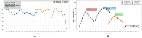
Figure 16. TSF-GRU model performance at Xidan station. (a) Passenger flow fitting: actual vs. predicted. (b) Prediction error analysis.

5. Discussion

Building on the empirical results in Section 4, this section conducts in-depth theoretical and practical discussions. It first interprets the mechanism behind the temporal differences in passenger flow and verifies the universality of the findings through cross-city comparisons. Then, it analyzes the dynamic evolution relationship between station roles and network bottlenecks, providing theoretical explanations for functional differentiation of stations. Finally, it discusses the practical value of the TSF-GRU model in refined subway operations, linking the research results to low-carbon development goals. This section aims to deepen the understanding of research findings, highlight the theoretical and practical significance of the study, and provide guidance for subsequent policy formulation and follow-up research.

5.1. Mechanism Interpretation of Temporal Differences and Cross-City Comparison

Subway passenger flows show distinct temporal patterns: weekday double peaks, holiday broad peaks, and weekend dispersed peaks. Weekday peaks arise from job–housing separation and fixed work schedules (08:00–09:00 and 18:00–19:00), while holiday and weekend flows reflect flexible leisure and social travel [1,2,3]. The temporal regularities observed in Beijing are broadly consistent with other urban rail systems. For example, Shenzhen’s metro exhibits bimodal weekday peaks and flatter or composite peaks on weekends and holidays [42], while London, Shanghai, and Tokyo show high-frequency travel intervals within 15–25 min, reflecting universal patterns in commuter behavior and socio-economic rhythms [12,14,28,43].

Despite these similarities, Beijing shows a higher proportion of interregional transfer flows on holidays and weekends, reflecting its role as a regional transportation hub with complex demand dynamics. This contextual difference underlines the importance of considering local infrastructure and socio-economic factors when interpreting temporal patterns. These cross-city comparisons not only validate the temporal characteristics identified in this study but also suggest that the proposed framework can inform similar analyses in other megacities with complex transport networks.

5.2. Time Variability of Station Roles and Network-Based Interpretation of Bottleneck Dynamics

Network analysis demonstrates that subway station roles vary significantly across temporal contexts and closely relate to bottleneck evolution. Transportation hubs concentrate flows on holidays and weekends, commuter-oriented stations dominate weekday peaks, and commercial–leisure stations gain prominence during non-working periods [8,44,45].

Weekday bottlenecks are primarily rigid, concentrated along commuting corridors (e.g., Xierqi and Chaoyangmen), driven by high-intensity unidirectional flows and structural network constraints. In contrast, holiday bottlenecks (e.g., Beijing West and Xidan) are flexible, arising from overlapping flows and fluctuating network capacities. Weekend bottlenecks combine these characteristics, reflecting residual commuting and leisure activities. Recognizing these differences is essential for effective operational planning, as it allows for targeted measures, such as peak-direction management for rigid bottlenecks and dynamic scheduling for flexible ones.

The dynamic relationship between station roles and bottleneck evolution highlights the interconnectedness of network topology, passenger behavior, and temporal demand. By linking these components, this study provides a coherent framework that integrates temporal patterns, functional differentiation, and bottleneck identification. This approach overcomes the limitations of isolated analyses and demonstrates how spatiotemporal insights can inform both theoretical understanding and practical subway management strategies.

5.3. Contributions of Spatiotemporal Fusion Prediction to Refined Operations

The TSF-GRU model enhances operational decision-making by combining temporal, spatial, and network topological features. It achieves a test-set MAPE of 7.62% and ≤3.4% accuracy under complex conditions, outperforming models relying solely on temporal patterns [3,22,34,46]. This integration allows for precise, differentiated strategies tailored to different station types, supporting dynamic train scheduling, personnel allocation, and capacity adjustment. Importantly, the predictive framework forms a logical chain with temporal feature analysis, station role classification, and bottleneck identification, validating its practical applicability. By bridging methodological advances in deep learning with real-world operational needs, the model provides a scalable, transferable technical pathway for both Beijing and other large-scale urban rail systems.

6. Conclusions

This study develops a dynamic temporal network framework to analyze subway passenger flows, node functional differentiation, and bottleneck dynamics, providing both theoretical insights and practical guidance for refined urban rail operations.

Regarding spatiotemporal flow patterns, the analysis reveals that weekday flows exhibit sharp double peaks, holiday flows present sustained broad peaks, and weekend flows feature extended and flexible peaks. These patterns reflect the diverse temporal distribution of urban travel demands and highlight the periodicity and variability of passenger flows under different day types. In terms of node functional differentiation, transportation hubs, commuter-oriented nodes, and commercial stations perform distinct temporal roles. Hubs primarily serve as passenger aggregation and distribution centers during holidays and weekends, commuter nodes dominate peak-hour weekday flows, and commercial stations gain prominence during leisure periods. This differentiation closely aligns with the spatial layout of urban functions and provides empirical insights into the organization of urban passenger flows. For bottleneck dynamics, weekday bottlenecks are rigid, primarily driven by high-intensity, unidirectional flows along commuting corridors. Holiday bottlenecks are flexible, arising from multi-source passenger flows and network capacity fluctuations. Weekend bottlenecks display mixed characteristics, reflecting a combination of leisure travel and residual commuting demand. These differentiated patterns offer guidance for targeted and dynamic management strategies tailored to each bottleneck type. The study also proposes a predictive framework using the TSF-GRU model, which integrates temporal, spatial, and network topological features. This model accurately forecasts station-level passenger flows, supporting real-time, differentiated operational strategies, and providing indirect support for low-carbon scheduling through more efficient capacity allocation and resource utilization.

Limitations of this study include the restricted dataset, which covers only a single holiday, weekend day, and weekday, potentially limiting robustness in capturing typical travel patterns. The analysis focuses primarily on node-level characteristics, while edge-level dynamics and external factors such as weather or special events are not fully incorporated. Moreover, the findings are context-specific to Beijing, and broader applicability to other megacities requires careful adaptation.

Future research directions are proposed to further extend this study. With increasing data complexity and the development of multimodal transportation systems, future work could incorporate artificial intelligence and machine learning approaches to enhance analytical capability. In particular, advanced spatiotemporal learning models, graph-based methods, and multimodal data fusion techniques could be explored to better capture complex spatiotemporal dependencies and interactions across transportation modes. Such extensions would improve the adaptability of the proposed framework to more complex urban mobility scenarios and further support refined and low-carbon operational decision-making.

References

- Feng, J.; Li, X.; Mao, B.; Xu, Q.; Bai, Y. Weighted Complex Network Analysis of the Beijing Subway System: Train and Passenger Flows. Phys. A Stat. Mech. Appl. 2017, 474, 213–223. [Google Scholar] [CrossRef]
- Leng, B.; Zeng, J.; Xiong, Z.; Lv, W.; Wan, Y. Probability Tree Based Passenger Flow Prediction and Its Application to the Beijing Subway System. Front. Comput. Sci. 2013, 7, 195–203. [Google Scholar] [CrossRef]
- Sun, Y.; Leng, B.; Guan, W. A Novel Wavelet-SVM Short-Time Passenger Flow Prediction in Beijing Subway System. Neurocomputing 2015, 166, 109–121. [Google Scholar] [CrossRef]
- Wang, Y.; Wang, Y.; Ettema, D.; Mao, Z.; Charlton, S.G.; Zhou, H. Commuter Value Perceptions in Peak Avoidance Behavior: An Empirical Study in the Beijing Subway System. Transp. Res. Part A Policy Pract. 2020, 139, 70–84. [Google Scholar] [CrossRef]
- Wang, G.; Liu, Y.; Hu, Z.; Zhang, G.; Liu, J.; Lyu, Y.; Gu, Y.; Huang, X.; Zhang, Q.; Liu, L. Flood Risk Assessment of Subway Systems in Subwaypolitan Areas Under Land Subsidence Scenario: A Case Study of Beijing. Remote Sens. 2021, 13, 637. [Google Scholar] [CrossRef]
- Wei, Y.; Liang, J.; Deng, Y.; Dou, F.; Ning, Y.; Zhou, D.; Liu, J. Resilience Assessment of Beijing Subway Lines under Extreme Precipitation Weather. Appl. Sci. 2023, 13, 3964. [Google Scholar] [CrossRef]
- Zhang, Z.; Fujii, H.; Managi, S. How Does Commuting Behavior Change Due to Incentives? An Empirical Study of the Beijing Subway System. Transp. Res. Part F Traffic Psychol. Behav. 2014, 24, 17–26. [Google Scholar] [CrossRef]
- Yang, Y.; Liu, Y.; Zhou, M.; Li, F.; Sun, C. Robustness Assessment of Urban Rail Transit Based on Complex Network Theory: A Case Study of the Beijing Subway. Saf. Sci. 2015, 79, 149–162. [Google Scholar] [CrossRef]
- Zheng, S.; Hu, X.; Wang, J.; Wang, R. Subways near the Subway: Rail Transit and Neighborhood Catering Businesses in Beijing. Transp. Policy 2016, 51, 81–92. [Google Scholar] [CrossRef]
- Zou, L.; Chen, Y.; Guo, R.; Wang, P.; He, Y.; Chen, S.; Wang, Z.; Zhu, J. Unraveling the Impact of COVID-19 on Beijing’s Subway System Using a Causal Machine Learning Analysis. Sustain. Cities Soc. 2025, 131, 106709. [Google Scholar] [CrossRef]
- Zhou, M.; Dong, H.; Wang, X.; Hu, X.; Ge, S. Modeling and Simulation of Crowd Evacuation with Signs at Subway Platform: A Case Study of Beijing Subway Stations. IEEE Trans. Intell. Transp. Syst. 2020, 23, 1492–1504. [Google Scholar] [CrossRef]
- Chen, C.; Chen, J.; Barry, J. Diurnal Pattern of Transit Ridership: A Case Study of the New York City Subway System. J. Transp. Geogr. 2009, 17, 176–186. [Google Scholar] [CrossRef]
- Cui, J.; Nelson, J.D.; Beecroft, M.; Lin, D. Subway Systems and Tourism: An Overview and Implications. Res. Transp. Bus. Manag. 2024, 57, 101205. [Google Scholar] [CrossRef]
- Lee, J.-H.; Goh, S.; Lee, K.; Choi, M.Y. Spatiotemporal Distributions of Population in Seoul: Joint Influence of Ridership and Accessibility of the Subway System. EPJ Data Sci. 2021, 10, 41. [Google Scholar] [CrossRef]
- Kim, H.; Song, Y. Examining Accessibility and Reliability in the Evolution of Subway Systems. J. Public Transp. 2015, 18, 89–106. [Google Scholar] [CrossRef]
- Lee, K.; Goh, S.; Park, J.S.; Jung, W.-S.; Choi, M. Master Equation Approach to the Intra-Urban Passenger Flow and Application to the Subwaypolitan Seoul Subway System. J. Phys. A Math. Theor. 2011, 44, 115007. [Google Scholar] [CrossRef]
- Lin, J.-J.; Gau, C.C. A TOD Planning Model to Review the Regulation of Allowable Development Densities around Subway Stations. Land Use Policy 2006, 23, 353–360. [Google Scholar] [CrossRef]
- Nagel, T.; Groß, B. Shanghai Subway Flow: Multiple Perspectives into a Subway System. Leonardo 2017, 50, 511–512. [Google Scholar] [CrossRef]
- Liu, X.; Macedo, J.; Zhou, T.; Shen, L.; Liao, Y.; Zhou, Y. Evaluation of the Utility Efficiency of Subway Stations Based on Spatial Information from Public Social Media. Habitat Int. 2018, 79, 10–17. [Google Scholar] [CrossRef]
- Su, S.; Tang, T.; Li, X.; Gao, Z. Optimization of Multitrain Operations in a Subway System. IEEE Trans. Intell. Transp. Syst. 2013, 15, 673–684. [Google Scholar] [CrossRef]
- Wei, D.; Zhang, H.; Tsang, W.; Gong, J.; Mei, Z. Investigating the Influencing Factors of Cooperation Between Shared E-Bikes and Subway Systems: A Multivariate Data Analysis. Transp. Policy 2025, 174, 103825. [Google Scholar] [CrossRef]
- Toto, E.; Rundensteiner, E.A.; Li, Y.; Jordan, R.; Ishutkina, M.; Claypool, K.; Luo, J.; Zhang, F. Pulse: A Real Time System for Crowd Flow Prediction at Subwaypolitan Subway Stations. In Proceedings of the Joint European Conference on Machine Learning and Knowledge Discovery in Databases, Riva del Garda, Italy, 19–23 September 2016; Springer: Berlin/Heidelberg, Germany, 2016; pp. 112–128. [Google Scholar]
- Yang, X.; Li, X.; Gao, Z.; Wang, H.; Tang, T. A Cooperative Scheduling Model for Timetable Optimization in Subway Systems. IEEE Trans. Intell. Transp. Syst. 2012, 14, 438–447. [Google Scholar] [CrossRef]
- Deng, Y.; Li, Q.; Lu, Y. A Research on Subway Physical Vulnerability Based on Network Theory and FMECA. Saf. Sci. 2015, 80, 127–134. [Google Scholar] [CrossRef]
- Angeloudis, P.; Fisk, D. Large Subway Systems as Complex Networks. Phys. A Stat. Mech. Appl. 2006, 367, 553–558. [Google Scholar] [CrossRef]
- Chen, J.; Liu, J.; Peng, Q.; Yin, Y. Resilience Assessment of an Urban Rail Transit Network: A Case Study of Chengdu Subway. Phys. A Stat. Mech. Appl. 2022, 586, 126517. [Google Scholar] [CrossRef]
- Derrible, S.; Kennedy, C. Network Analysis of World Subway Systems Using Updated Graph Theory. Transp. Res. Rec. 2009, 2112, 17–25. [Google Scholar] [CrossRef]
- Lee, K.; Jung, W.-S.; Park, J.S.; Choi, M.Y. Statistical Analysis of the Subwaypolitan Seoul Subway System: Network Structure and Passenger Flows. Phys. A Stat. Mech. Appl. 2008, 387, 6231–6234. [Google Scholar] [CrossRef]
- Han, C.; Liu, L. Topological Vulnerability of Subway Networks in China. In Proceedings of the 2009 International Conference on Management and Service Science, Beijing, China, 20–22 September 2009; IEEE: New York City, NY, USA, 2009; pp. 1–4. [Google Scholar]
- Yu, L.; Cui, M. How Subway Network Affects Transit Accessibility and Equity: A Case Study of Xi’an Subwaypolitan Area. J. Transp. Geogr. 2023, 108, 103556. [Google Scholar] [CrossRef]
- Kim, H. Geographical Analysis on Network Reliability of Public Transportation Systems: A Case Study of Subway Network System in Seoul: A Case Study of Subway Network System in Seoul. J. Korean Geogr. Soc. 2009, 44, 187–205. [Google Scholar]
- Liu, Y.; Tan, Y. Complexity Modeling and Stability Analysis of Urban Subway Network: Wuhan City Case Study. Procedia-Soc. Behav. Sci. 2013, 96, 1611–1621. [Google Scholar] [CrossRef]
- Park, J.-S.; Lee, K.-S. Network Structures of the Subwaypolitan Seoul Subway Systems. J. Econ. Geogr. Soc. Korea 2008, 11, 459–475. [Google Scholar] [CrossRef]
- M’cleod, L.; Vecsler, R.; Shi, Y.; Levitskaya, E.; Kulkarni, S.; Malinchik, S.; Sobolevsky, S. Vulnerability of Transportation Networks: The New York City Subway System under Simultaneous Disruptive Events. Procedia Comput. Sci. 2017, 119, 42–50. [Google Scholar] [CrossRef]
- Semaan, N. Structural Performance Model for Subway Networks. Ph.D. Thesis, Concordia University, Montreal, QC, Canada, 2011. [Google Scholar]
- Roth, C.; Kang, S.M.; Batty, M.; Barthelemy, M. Evolution of Subway Networks. Cities 2012, 20, 40. [Google Scholar]
- Song, J.; Abuduwayiti, A.; Gou, Z. The Role of Subway Network in Urban Spatial Structure Optimization–Wuhan City as an Example. Tunn. Undergr. Space Technol. 2023, 131, 104842. [Google Scholar] [CrossRef]
- Yang, Y.; Huang, A.; Guan, W. Statistic Properties and Cascading Failures in a Coupled Transit Network Consisting of Bus and Subway Systems. Int. J. Mod. Phys. B 2014, 28, 1450212. [Google Scholar] [CrossRef]
- Xu, Q.; Mao, B.H.; Bai, Y. Network Structure of Subway Passenger Flows. J. Stat. Mech. Theory Exp. 2016, 2016, 033404. [Google Scholar] [CrossRef]
- Zhou, Z.; Li, J.; Chen, Z.; Huang, Z.; Pan, Y.; Sun, C. Using Urban Subway Network System for Freight Transportation in Consideration of Passenger Safety. Comput. Ind. Eng. 2025, 211, 111571. [Google Scholar] [CrossRef]
- Zhang, J.; Xu, X.; Hong, L.; Wang, S.; Fei, Q. Networked Analysis of the Shanghai Subway Network, in China. Phys. A Stat. Mech. Appl. 2011, 390, 4562–4570. [Google Scholar] [CrossRef]
- Mao, R.; Ji, X.; Yin, A.; Chen, F.; Zhao, R. Characteristics and Comparison of Spatiotemporal Dynamic Fluctuation of Subway Passenger Flow: A Case Study of Shenzhen. Trop. Geogr. 2024, 44, 1210–1222. [Google Scholar] [CrossRef]
- Zheng, Y.Y.; Takayasu, H.; Takayasu, M. Do Railway Commuters Exhibit Consistent Route Choice Rationality Across Different Contexts and Time? Evidence from Tokyo Metropolitan Commutes. arXiv 2025, arXiv:2510.12381. [Google Scholar] [CrossRef]
- Wang, Z.; Zhang, M. Spatio-temporal Evolution Characteristics of Beijing Subway Network and Its Evolution Mechanism. Econ. Geogr. 2021, 41, 48–56. [Google Scholar] [CrossRef]
- Zhou, Y.; Wang, H.; Chen, S.; Jiang, J.; Wang, Z.; Liu, W. Investigating Holiday Subway Travel Flows with Spatial Correlations Using Mobile Payment Data: A Case Study of Hangzhou. Sustainability 2025, 17, 5873. [Google Scholar] [CrossRef]
- Zhang, S.; Zhang, J.; Yang, L.; Yin, J.; Gao, Z. Spatial-Temporal Attention Fusion Network for Short-Term Passenger Flow Prediction on Holidays in Urban Rail Transit Systems. arXiv 2022, arXiv:2203.00007. [Google Scholar]
Disclaimer/Publisher’s Note: The statements, opinions and data contained in all publications are solely those of the individual author(s) and contributor(s) and not of MDPI and/or the editor(s). MDPI and/or the editor(s) disclaim responsibility for any injury to people or property resulting from any ideas, methods, instructions or products referred to in the content. |
© 2026 by the authors. Licensee MDPI, Basel, Switzerland. This article is an open access article distributed under the terms and conditions of the Creative Commons Attribution (CC BY) license.