Dual Perspectives: Safety Assessment of Legacy Pillars via Numerical Simulation and Artificial Intelligence Techniques

Abstract

The long-term stability of legacy pillars remains a critical challenge in mining engineering, as pillar collapse may threaten human safety, damage infrastructure, and complicate sustainable mine closure. Conventional empirical methods are often inadequate for addressing the complexity of heterogeneous rock masses and time-dependent deterioration. In this study, a dual-perspective framework is proposed by integrating finite difference method (FDM)-based numerical simulation with artificial intelligence (AI) techniques to improve the reliability of pillar safety assessment. FDM models are developed to analyze stress redistribution, deformation, and failure processes of pillars under varying depths, geometries, rock quality, and rock mechanics. In parallel, AI models are trained on datasets derived from numerical simulations to provide rapid predictions of pillar instability probability (P_f) with high computational efficiency. The complementary use of both approaches ensures cross-validation: FDM simulations provide mechanistic insights into pillar behavior, while AI models enhance predictive capability and account for uncertainties in geological conditions. The integrated framework demonstrates superior robustness and applicability compared to single-method approaches, offering a comprehensive tool for assessing legacy pillar safety. This research provides practical guidance for hazard mitigation, mine closure planning, and the development of monitoring strategies in sustainable mining engineering.

1. Introduction

Continuous industrial expansion has led to a sustained increase in the consumption of metallic resources, while shallow and easily exploitable deposits have been extensively exhausted over time [1,2,3]. Under these circumstances, underground extraction has become the dominant mode for metal mining across many regions. Unlike surface operations, underground mining is characterized by confined spaces and complex stress environments, where structural instability may pose serious threats to personnel safety and operational continuity [4]. To preserve the integrity of underground openings, pillars are commonly left in place during excavation. However, many existing underground mines contain a substantial number of legacy pillars that were formed decades ago under outdated design concepts, limited geological information, and insufficient monitoring practices. Prolonged service, damage accumulation, and uncertainty in material properties further complicate the evaluation of their load-bearing capacity [5]. Consequently, the stability of underground excavations is strongly dependent on the condition of these legacy pillars, highlighting the urgent need for reliable and robust safety assessment approaches.

Over the past decades, various approaches have been developed to evaluate pillar stability, including empirical design methods, numerical simulations, and data-driven techniques. These approaches have contributed significantly to the understanding and assessment of pillar behavior under different geological and mining conditions. However, in practical engineering applications, the stability of legacy hard rock pillars is governed by the combined effects of stress conditions, geometry, material properties, and rock mass quality, and is often accompanied by substantial uncertainty. This inherent complexity makes pillar safety assessment a challenging task that cannot be fully characterized from a single analytical perspective. In engineering decision-making, insufficient consideration of instability risk may lead to unsafe conditions, while overly conservative judgments may result in unnecessary reinforcement or rehabilitation measures. Therefore, an assessment methodology that provides both physically meaningful insight and probabilistic risk quantification is essential for informed hazard mitigation and sustainable underground mining operations. Despite extensive research on pillar stability, existing assessment practices still lack a unified framework that (i) explicitly incorporates rock mass quality, (ii) evaluates pillar instability from a probabilistic perspective, and (iii) enables efficient yet physically consistent assessment of legacy pillars under uncertain geological conditions. In particular, the role of rock mass quality in modifying pillar behavior and instability risk has not been sufficiently integrated into probabilistic evaluation frameworks.

To address these issues, this study presents a dual-perspective framework for the safety assessment of legacy hard rock pillars by integrating numerical simulation and Artificial intelligence (AI) techniques. Physics-based numerical simulations are employed to characterize pillar mechanical behavior under varying rock mass conditions, while machine learning (ML) models are developed to estimate pillar instability probability in a probabilistic manner. Rock mass quality, represented by the Geological Strength Index (GSI), is explicitly incorporated to enhance the physical relevance of both approaches. Furthermore, metaheuristic optimization algorithms are introduced to improve the predictive performance and robustness of the machine learning models. Through this integrated strategy, the proposed framework aims to provide a more reliable and practical tool for probabilistic stability evaluation of legacy pillars.

2. Related Work and Literature Review

Owing to the critical role of pillars in maintaining excavation integrity and ensuring operational safety, a variety of analytical approaches have been developed to evaluate their stability. In general, three categories of methods are most commonly employed: empirical deterministic approaches based on strength formulas, physics-based numerical simulation techniques, and data-driven artificial intelligence methods [6]. Empirical deterministic methods represent the earliest and most widely adopted approach for evaluating pillar stability. These methods typically estimate pillar stability by calculating a safety factor (SF), defined as the ratio between pillar strength and the applied stress, where pillar strength is expressed as an empirical function of geometric dimensions and material strength [7]. Numerous studies refined and validated pillar strength formulas under different coal mining conditions, yielding generally satisfactory predictions within their respective applicability ranges [8,9,10,11]. Compared with coal pillars, the mechanical behavior of hard rock pillars is more complex, which significantly complicates the development of reliable empirical strength formulas. Hedley and Grant [12] introduced one of the earliest strength equations specifically developed for hard rock pillars and successfully applied it to the stability assessment of 28 pillars in the Elliot Lake uranium mine. However, the governing variables are still largely restricted to pillar dimensions and intact rock strength [13]. Extensive engineering experience has shown that such empirical formulas are often valid only for specific mines and geological settings, and their direct transferability to other sites is limited. This lack of general applicability suggests that important controlling factors influencing hard rock pillar stability are not adequately captured by purely empirical formulations. Although later studies incorporated rock mass quality indicators to improve strength estimation—such as modifying intact rock strength using rock mass classification systems [14,15]. Nevertheless, empirical approaches remain fundamentally limited in their ability to describe stress redistribution, deformation evolution, and progressive failure processes. These limitations have driven increasing interest in physics-based numerical simulation techniques [16].

Kortnik [17] emphasized that the numerical simulations offer a more comprehensive depiction of hard rock pillar behavior than empirical methods, and allow the progressive evolution of stability to be examined under varying stress environments. Numerous studies have demonstrated the capability of numerical methods to investigate key factors controlling pillar stability [18,19,20]. Mortazavi et al. [21] used FLAC to model hard rock pillars under in situ stress conditions and showed that pillar geometry, particularly the width-to-height ratio (w/h), plays a dominant role during the initial stages of pillar deformation and governs subsequent failure development. Renani and Martin [22] conducted both two-dimensional (2D) and three-dimensional (3D) finite-difference analyses on 85 pillar cases, revealing that pillars with values of w/h below 2.0 exhibit strain-softening behavior, whereas wider pillars tend to show hardening responses. Their results further suggested that empirical strength formulas may overestimate pillar strength under certain conditions. Kim et al. [23] constructed numerical models of stopes containing multiple pillars and demonstrated that pillar arrangement significantly influences overall excavation stability, as evidenced by variations in SF, displacement, stress distribution, and plastic zone development. Kumar et al. [24] incorporated strain-softening behavior into numerical models and calibrated simulations using empirical strength formulas that account for pillar depth and in situ monitoring data, achieving good agreement between numerical predictions and field observations. Despite their advantages in revealing mechanical mechanisms, numerical simulation methods are computationally intensive and time-consuming, particularly for large-scale or site-specific analyses [5,25]. In addition, simplifications in geometry and boundary conditions are often required, which may introduce discrepancies between simulated and actual pillar behavior [26].

AI methods have emerged as a promising alternative for pillar stability assessment, particularly in situations where rapid evaluation is required and large datasets are available [27,28,29]. AI-based approaches typically rely on databases composed of pillar geometric parameters, mechanical properties, and stress-related variables, from which ML algorithms are trained to identify patterns and predict stability states. Ghasemi et al. [30] applied several intelligent classification algorithms to a dataset of 178 hard rock pillars and demonstrated that both J48 decision trees and support vector machines (SVM) achieved high prediction accuracy, with the J48 model outperforming traditional regression approaches. Idris et al. [31] employed artificial neural networks (ANN) to predict pillar strain responses based on numerical simulation results and combined this approach with Monte Carlo (MC) analysis to assess pillar reliability, showing that pillar’s w/h ratio plays a critical role in stability and that reliability increases with increasing ratio. Ding et al. [32] used stochastic gradient boosting (SGB) to classify pillar stability and identified pillar stress (Ps) and w/h ratio as the most influential variables. Zhou et al. [33] compared Fisher discriminant analysis and SVM for pillar stability prediction and found that support vector machines provided superior performance. With the expansion of available datasets, Zhou et al. [34] evaluated six classification algorithms using 251 hard rock pillar cases and concluded that SVM and random forest (RF) models yielded the best overall performance, while emphasizing the importance of Ps, geometry, and stress-related inputs. Qiu and Zhou [35] proposed a novel gene-expression programming (HGEP) model to predict the probability of hard rock pillars. They determined the pillar condition based on a new evaluation index named the hard rock pillar stability index (HPSI). Li et al. [36] developed a Logistic model tree (LMT) to predict the stability of rock and coal pillars. Although numerous ML models have been developed to predict pillar stability, the input features used in existing databases are still largely limited to Ps, w/h, burial depth (H), and uniaxial compressive strength (UCS). Rock mass quality indices that have a significant influence on pillar strength, such as the GSI, have received relatively little attention. Li et al. [37] proposed a novel empirical formula considering GSI and other traditional features to calculate pillar strength and evaluate the pillar stability. The study revealed that the GSI exerts a stronger influence on sloughing pillars than on stable or failed hard rock pillars. Moreover, the stability of most pillars is typically assessed based on the SF, whereas in practice, pillars with low SF values may still remain stable. Therefore, evaluating pillar stability from a probabilistic perspective represents a worthwhile direction for further investigation. Wattimena et al. [38] similarly demonstrated the applicability of logistic regression for estimating pillar stability probabilities. Wattimena [39] applied multiclass logistic regression (MLR) to estimate the probabilities of different pillar stability states, reporting an overall prediction accuracy of 79.21%, which suggests that such models can be effective for preliminary stability screening. In conclusion, the safety assessment of pillar stability still faces the following challenges:

(1) Probabilistic investigation of hard rock pillar stability that integrates numerical simulation and ML remains largely unexplored, particularly when rock mass quality parameters such as the GSI are explicitly considered.

(2) Existing ML studies on pillar instability probability are still limited, and metaheuristic optimization algorithms have rarely been employed to enhance model performance and robustness.

3. Methodologies

3.1. Integrated Numerical Simulation and AI Framework

This study adopts an integrated numerical simulation and AI framework to assess the instability probability of legacy hard rock pillars. Numerical simulations are first conducted to characterize pillar mechanical behavior and generate physically consistent stability indicators under varying geological and geometric conditions. These simulation results are subsequently used to construct a dataset for training AI models, enabling efficient probabilistic prediction of pillar instability.

3.1.1. Numerical Simulation and Data Generation

Numerical simulation was performed to analyze the mechanical behavior and stability of hard rock pillars under representative excavation and stress conditions in this study. All simulations were conducted using FLAC3D (version 5.0), which employs an explicit finite-difference formulation suitable for modeling nonlinear rock mass behavior and progressive failure. As shown in Figure 1, a 3D pillar model was constructed to represent a realistic underground mining scenario, explicitly including the pillar and surrounding rock mass. To minimize boundary effects, the model dimensions were selected to be significantly larger than the excavation span, with a horizontal extent of approximately 160 m and a vertical extent of 80 m. Boundary conditions were applied by fixing the bottom boundary, constraining lateral boundaries in the normal direction, and leaving the upper boundary free, allowing vertical loading while avoiding artificial stress concentration. The pillar material was modeled using a strain-softening constitutive model to capture post-peak strength degradation and progressive damage, while the surrounding rock mass and ore body were assumed to behave elastically. Material parameters were assigned to represent rock mass conditions, with the influence of rock mass quality incorporated through parameter selection informed by the GSI. Pillar loading was estimated using the tributary area theory, in which each pillar supports the weight of the overlying rock mass within its tributary area. Accordingly, the applied vertical stress was determined as a function of overburden thickness, rock density, pillar width, and excavation span. The numerical modeling framework was designed to systematically examine the influence of UCS, GSI, w/h, stope span (B), and H on hard rock pillar stability.

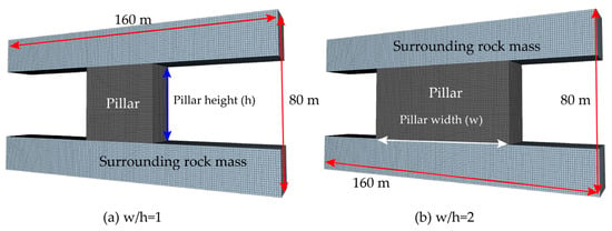
Figure 1. Numerical simulation demonstration of pillars with different geometric conditions.

Accordingly, two complementary indicators were extracted from the numerical simulation results to evaluate pillar stability. First, a deterministic strength–stress ratio (i.e., SF) was obtained at the element level based on the constitutive response. Elements with a strength–stress ratio below a critical threshold (1.5 was set in this study) were identified as unstable, enabling visualization of stress concentration and failure-prone regions within the pillar. Second, the plastic zones can be adopted to characterize progressive pillar failure [40]. Plastic yielding represents irreversible damage, and its spatial extent provides insight into the degradation state of the pillar. To enable probabilistic interpretation, the ratio of plastic elements to the total number of pillar elements was calculated and interpreted as an instability probability (P_f). The mathematical formulation is presented in Equation (1).

$${\mathrm{P}}_{\mathrm{f}}={\displaystyle \frac{Z_n}{Z_t}}\times 100\%\left(n=1,\dots ,t\right)$$

(1)

where P_f denotes the probability of pillar instability, Z_n represents the number of plastic elements, and Z_m denotes the total number of elements of the pillar.

3.1.2. AI Model Training and Prediction Task

To bridge physics-based analysis and data-driven prediction, numerical simulation and AI were integrated into a unified framework for probabilistic stability assessment of hard rock pillars. Numerical simulation provides physically consistent stability indicators, while ML model learns the nonlinear relationship between governing parameters and pillar instability probability, enabling efficient and interpretable prediction. As shown in Figure 2, the framework was organized as following parts:

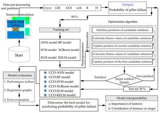
Figure 2. Flowchart of combining numerical simulation with AI to predict pillar stability.

(1) Numerical validation: Before coupling numerical simulation with ML, the reliability of the numerical model was first examined using representative pillar cases. For these benchmark cases, numerical simulations were conducted using the same geometric configurations and mechanical conditions as documented in the original studies. The numerically calculated pillar strength was then compared with the corresponding actual values.

(2) Data generation: Following numerical validation, the verified simulation framework was used to generate a database for developing ML models. A series of numerical simulations was performed under varying operating conditions to systematically investigate the combined influence of UCS, GSI, w/h, B, and H on pillar stability. By varying these parameters within representative ranges, a total of 100 numerical simulation cases were conducted.

(3) Model construction: Based on the generated dataset, ML models were developed to predict pillar instability probability. Prior to model training, all input features were normalized to eliminate the influence of differing units and magnitudes on model performance. The dataset was then randomly divided into training and test subsets with a ratio of 8:2, ensuring that model evaluation was conducted using unseen data. To promote robust generalization and ensure fair comparison among different learning algorithms, all ML models were trained under a unified model complexity control and validation strategy. Hyperparameters governing model structure and learning behavior were automatically tuned using the Cuckoo Catfish Optimizer (CCO). Although hyperparameter optimization does not constitute explicit regularization, it enables the selection of appropriately constrained model configurations, thereby implicitly mitigating overfitting within the physically bounded parameter space defined by the numerical simulation. Model performance was subsequently evaluated using multiple criteria, including the coefficient of determination (R²), root mean square error (RMSE), variance accounted for (VAF), and mean absolute error (MAE). Regression plots and error distribution analyses were employed to further assess model accuracy and robustness, allowing a comprehensive comparison among different learning algorithms.

(4) Model interpretability: To enhance interpretability and gain insight into the contribution of individual input features, Shapley additive explanations (SHAP) analysis was applied to the trained ML models. SHAP values were used to quantify the contribution of each input feature (UCS, GSI, w/h, B, and H), to the predicted pillar instability probability at both global and local levels.

In this study, ML models are trained to approximate the outputs of a physics-based numerical simulation rather than to directly predict raw field behavior. The numerical model acts as an intermediary that represents rock mass response through constitutive laws, stress redistribution, and failure criteria defined by geomechanical principles. Field uncertainty is reflected through the selection of realistic parameter ranges that bound plausible geological and mechanical conditions. As a result, the predicted instability probability should be interpreted as a scenario-based indicator supporting engineering decision-making, rather than as a direct prediction of in situ behavior. It should be emphasized that the machine learning models employed in this study are not intended to replace deterministic numerical simulations, but to serve as computationally efficient surrogate predictors of the FLAC3D response surface within a physically bounded parameter space.

3.2. Artificial Intelligence

3.2.1. ML Models

To represent different learning mechanisms and model complexities in pillar instability probability prediction, six ML models were adopted in this study, namely ANN, RF, SVM, extreme gradient boosting (XGBoost), extreme learning machine (ELM), and kernel extreme learning machine (KELM). ANN employs layered nonlinear transformations formed by interconnected neurons, allowing flexible mapping between input features and target responses in strongly coupled systems [41]. RF constructs multiple decision trees using randomized sampling and feature partitioning, and aggregates their outputs to achieve stable prediction performance under data uncertainty [42]. SVR formulates regression as a margin-based optimization problem, where kernel functions enable nonlinear relationships to be captured within a controlled error tolerance [43]. XGBoost builds tree-based models in a sequential manner by iteratively correcting residuals, while incorporating regularization terms to balance model complexity and predictive capability [44]. ELM adopts a single hidden-layer structure in which internal parameters are randomly assigned and output weights are directly solved, resulting in high computational efficiency [45]. KELM further enhances this framework by replacing explicit hidden-layer mapping with kernel functions, thereby strengthening nonlinear representation without increasing training burden [46]. It should be noted that the predictive performance of each ML model is closely related to the selection of hyperparameters. The hyperparameters of each model and their corresponding setting ranges are listed in Table 1.

Table 1. Setting of hyperparameters for all ML models.

Models	Hyperparameters	Description	Range
ANN	Nh	The number of hidden layers	[1, 3]
	Nn	The number of neurons in a hidden layer	[1, 10]
RF	Nt	The number of trees	[1, 100]
	Minleaf	The minimum number of samples required to be at a leaf node	[1, 10]
SVM	C	Regularization parameter	[0.125, 256]
	kp	Kernel parameter	[0.125, 16]
XGBoost	Ne	The number of base estimators	[50, 200]
	Lr	The learning rate	[0.1, 1.0]
	Maxdepth	The maximum depth of each tree	[1, 30]
ELM	Nn	The number of neurons in a hidden layer	[1, 150]
KELM	C	Regularization parameter	[0.125, 256]
	kp	Kernel parameter	[0.125, 16]

3.2.2. Optimization Algorithm

In this study, the CCO developed by Wang et al. [47] was adopted to optimize all ML models. As a metaheuristic algorithm, these swarm intelligence–based approaches leverage collective behaviors emerging from simple agent interactions to address complex optimization problems [48,49,50]. For the CCO, the optimization process is driven by a hierarchical swarm mechanism that dynamically balances global exploration and local exploitation through cooperative interaction and adaptive disturbance. By progressively restricting the effective search region, guiding individuals to encircle promising areas, and introducing controlled stochastic perturbations near elite solutions, the algorithm enhances convergence accuracy while maintaining population diversity. The optimization process can be divided as follows:

(1) Initialization strategy: Before searching for food, the CCO needs to initialize the positions of individuals in the population. The initial positions of individuals are determined according to Equation (2):

$$C_i=rand\cdot (Ub-Lb)+Lb$$

(2)

where C_i represents the initial position of the i-th Cuckoo catfish in group. U_b and L_b are the upper and lower boundaries of searching space, respectively.

(2) Compressed space strategy: In this strategy, cooperative interactions are employed to progressively compress the effective search region, thereby limiting redundant exploration. At early iterations, individuals exploit collective spatial cues to form a coarse contraction, while subsequent updates apply more localized restrictions as population information accumulates. The corresponding position update mechanisms are mathematically formulated as follows:

$$C_i^{new}=C_i+Z_1\cdot \left|rd\right|\cdot \left({\displaystyle \frac{C_{best}+C_{r1}}{2}}-C_{r2}\right)+0.5r_3\cdot (C_{r3}-C_{r4})$$

(3)

$$C_i^{new}=Z_2\cdot (C_{i1}+\left|rd\right|\cdot (C_{i1}-C_{i2}))+(1-Z_2)\cdot C_i$$

(4)

$$C_i^{new}=C_{r1}+\left|rd\right|\cdot (C_{best}-C_i+C_{r2}-C_{r3})$$

(5)

where $C_i^{new}$ represent the updated position of the i-th Cuckoo catfish. Z₁ and Z₂ are two variables within the range of [0, 1]. $C_{best}$ represents the best position of Cuckoo catfish. $C_{r1}$, $C_{r2}$, $C_{r3}$, and $C_{r4}$ are the positions of random Cuckoo catfish in group. $\left|rd\right|$ is a factor with a normal distribution. $C_{i1}$ and $C_{i2}$ represent the positions of the i-th Cuckoo catfish in 1-dimensional and 2-dimensional, respectively.

(3) Surround search strategy: As shown in Figure 3, this strategy enables individuals to explore promising regions through encircling motions that combine peer-based information exchange with directional movement toward favorable positions. The corresponding position update process is mathematically defined as follows:

$$C_i^{new}=\left\{\begin{array}{ll}{C}_e+F\cdot R_1\cdot 0.5step+T^n\cdot s\cdot (1-R_1)\cdot \left|step\right|+V\cdot J_i/It& \mathrm{mod}(i,2)=0\\ C_e+F\cdot R_1\cdot 0.5step+T^n\cdot c\cdot (1-R_1)\cdot \left|step\right|+V\cdot J_i/It& otherwise\end{array}\right.$$

(6)

where C_e presents the reference position used as the center of the encircling motion. F is a direction factor within the range of [−1, 1]. s and c are two logarithmic helix coefficients. T is a shrinkage factor, and n is the shrinkage efficiency of the encirclement. $R_1$ represents the 1-dimensional random perturbation. V is movement speed of Cuckoo catfish. J_i represents the initial average aggregation degree of the i-th Cuckoo catfish. It is the number of iterations.

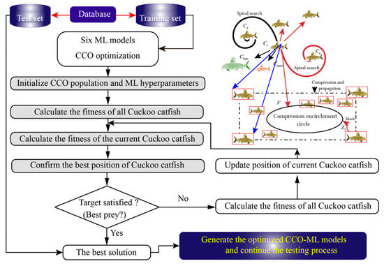
Figure 3. Optimization process of CCO algorithm for selecting the optimal hyperparameters of all ML models.

(4) Spherical wrap-around strategy: Each individual explores the search space by rotating around an adaptively defined center derived from elite solutions and collective population information (see Figure 3). The resulting spherical position update mechanism is mathematically expressed as follows:

$$C_i^{new}=\left\{\begin{array}{ll}Rot{C}_r+2\cdot w\cdot F\cdot \cos (R{t}_1)\cdot \sin (R{t}_2)\cdot (Rot{C}_r-C_i^{new})& C_q=1\\ Rot{C}_r+2\cdot w\cdot F\cdot \sin (R{t}_1)\cdot \cos (R{t}_2)\cdot (Rot{C}_r-C_i^{new})& C_q=2\\ Rot{C}_r+2\cdot w\cdot F\cdot \cos (R{t}_1)\cdot (Rot{C}_r-C_i^{new})& C_q=3\end{array}\right.$$

(7)

where $Rot{C}_r$ represents the predefined set of candidate spherical centers. w is a factor used for controlling the surround radius. Rt represents the rotation angle within the range of [0, 360]. C_q is a randomly generated discrete variable, which was set equal to 1, 2, and 3 in this algorithm.

4. Results and Discussion

This section presents and discusses the results obtained from the numerical simulation and AI analyses conducted in this study. The stability behavior of hard rock pillars is first examined from a physics-based perspective using numerical simulations, followed by probabilistic prediction and interpretation based on ML models.

4.1. Numerical Simulation

Numerical simulation results were analyzed to investigate the stability behavior of hard rock pillars under different GSI systems. Three representative rock mass quality levels were considered, corresponding to low (GSI = 25), medium (GSI = 55), and high (GSI = 85) conditions. For each GSI system, the influence of conventional controlling parameters (UCS, w/h, B, and H) on pillar stability was systematically examined. Pillar stability was evaluated using the strength–stress ratio and the proportion of yielded elements (i.e., SF and P_f), which was interpreted as pillar instability probability.

4.1.1. Numerical Validation for Pillar Model

To verify the reliability of the numerical pillar model, two representative hard rock pillar cases reported by Li et al. [37] with different geological and geometric conditions were simulated and compared with reference results. As illustrated in Figure 4a,b, the simulated stress–strain curves reproduced the typical elastic–plastic response and post-peak strain-softening behavior of hard rock pillars, and the numerically obtained peak strengths (67.7 MPa and 47.6 MPa) were consistent with expected values (71.3 MPa and 43.2 MPa). The model correctly estimated the pillar strength, confirming that the adopted numerical framework is suitable for subsequent parametric analysis and data generation for probabilistic stability assessment.

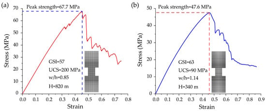
Figure 4. Numerical validation for pillar model based on two published cases.

4.1.2. Effect of UCS Under Different GSI Systems

To examine the influences of UCS on pillar stability in poor rock mass conditions, a series of cases were simulated at GSI = 25 with constant geometry and external conditions (w/h = 2, B = 20 m, H = 500 m) while varying UCS from 50 to 200 MPa. When UCS = 50 MPa, the pillar exhibited extensive yielding with 364 yielded elements, corresponding to P_f = 91%. As shown in Figure 5a, the plastic zone formed a continuous, shear-dominated through-going pattern (an “X-shaped” connectivity), and the high-risk region defined by SF < 1.5 overlapped strongly with the plastic zone, indicating a failed pillar state (see Figure 5b). For UCS = 100 MPa, the plastic zone element count decreased to 166 and P_f = 41.5%. As illustrated in Figure 5c, although the plastic zone was no longer fully through-going, it remained concentrated along the pillar sides, implying a non-negligible risk of local sloughing or partial collapse in practice. It can be seen from Figure 5d that the SF < 1.5 zone showed a similar side-concentrated distribution. Moreover, for UCS = 150 MPa, the plastic zone elements further decreased to 110 with P_f = 27.5% (see Figure 5e), and the high-risk SF region shown in Figure 5f remained localized without forming a continuous failure path. As shown in Figure 5g, plastic zone reduced to 74 elements and P_f = 18.5% when UCS equaled to 200 MPa, with the plastic zone mainly confined near pillar corners and excavation boundaries. Correspondingly, the SF < 1.5 region markedly shrank, supporting a stable-to-low-risk condition under this setting, as demonstrated in Figure 5h. In general, an increase in UCS significantly reduced the P_f of pillars when the rock mass quality of the pillar remained constant.

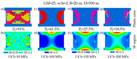
Figure 5. Impact of UCS on pillar stability under constant rock mass quality (GSI = 25).

To isolate the influence of rock mass quality, pillar responses under GSI = 25, 55, and 85 were compared at the same external conditions (UCS = 50 MPa, w/h = 2, B = 20 m, H = 500 m). The number of plastic zones and the characteristics of the SF regions for a pillar with GSI = 25. The failure state of the pillar at GSI = 55 is shown in Figure 6a, where the number of plastic zone elements in the pillar is 216 (i.e., P_f = 54%). As illustrated in Figure 6b, the SF < 1.5 region and plastic zone were primarily located along both pillar sides and tended to propagate toward the center but did not form a complete through-going path, corresponding to a moderate instability risk. At GSI = 85, the plastic zone elements reduced markedly to 96 (see Figure 6c) and Pf = 24%. As demonstrated in Figure 6d, both the plastic zone and SF < 1.5 region became much more limited and side-localized, indicating a substantially enhanced resistance against instability.

Figure 6. Impact of GSI on pillar stability for fixed operating conditions (UCS = 50 MPa, w/h = 2, B = 20 m, H = 500 m).

4.1.3. Effect of w/h Under Different GSI Systems

The influence of pillar geometry was evaluated by varying w/h under the GSI = 55 system at UCS = 100 MPa and H = 500 m (with the same stope configuration used in Figure 4 and Figure 5). When w/h = 0.5, the model produced 72 plastic zone elements and a high P_f = 72%, accompanied by a through-going shear-dominated plastic zone (see Figure 7a). As shown in Figure 7b the SF < 1.5 region was spatially consistent with this connected failure pattern, indicating an unstable state. It can be seen from Figure 7c that the plastic zone element number was 130 and P_f = 65% when w/h equal to 1. The plastic zone was still concentrated near both sides and remained associated with the SF < 1.5 region, implying persistent instability potential (see Figure 7d). With further increase to w/h = 2, plastic zone remained observable (136 elements shown in Figure 7e) but P_f decreased to 34%. As illustrated in Figure 7f, the SF < 1.5 region became restricted to small side portions and no longer indicated a through-going path, suggesting an overall stable condition. As demonstrated in Figure 7g,h, plastic zone reduced to 86 elements and P_f = 14.3% for w/h = 3, and both the plastic zone and SF < 1.5 region were minimal and localized, consistent with a robustly stable pillar.

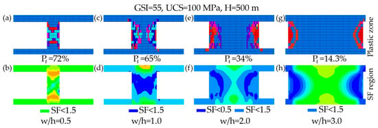
Figure 7. Impact of w/h on pillar stability under constant rock mass quality (GSI = 55).

A further comparison was performed for a consistent configuration (UCS = 100 MPa, w/h = 2, B = 20 m, H = 500 m) across the three GSI systems. As shown in Figure 8a,b, the low GSI case (GSI = 25) produced 176 plastic zone elements and P_f = 44%, with the plastic zone and SF < 1.5 region approaching a near-connected pattern, indicating a high likelihood of instability. Under GSI = 55, plastic zone decreased to 136 elements (see Figure 8c) and P_f = 34%, and the SF < 1.5 region remained side-localized without forming connectivity, indicating a stable state (see Figure 8d). As demonstrated in Figure 8e,f, the pillar exhibited only 58 plastic zone elements with P_f = 14.5% under GSI = 85, and the SF < 1.5 region was the smallest among the three, confirming that improved rock mass quality substantially suppresses instability under identical external loading and geometry.

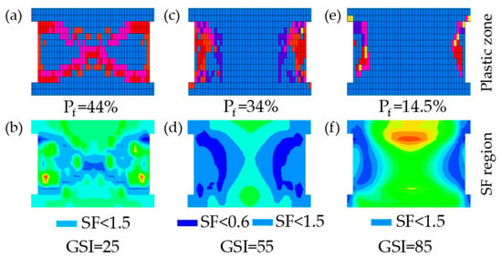
Figure 8. Impact of GSI on pillar stability for fixed operating conditions (UCS = 100 MPa, w/h = 2, B = 20 m, H = 500 m).

4.1.4. Effect of H Under Different GSI Systems

The destabilizing role of increasing in situ stress was examined by varying burial depth under GSI = 55, UCS = 150 MPa, and w/h = 2. As shown in Figure 9a, the pillar exhibited 70 plastic zone elements and P_f = 17.5% at H = 500 m. As illustrated in Figure 9b, the SF < 1.5 region was limited to small side portions and coincided with a localized plastic zone, indicating a low-risk condition. Increasing depth to H = 600 m increased plastic zone to 137 elements and P_f = 34.3% (see Figure 9c), and the SF < 1.5 zone expanded and remained consistent with the enlarged plastic zone (see Figure 9d), reflecting a clear rise in instability risk. It can be observed from Figure 9e that the plastic zone further increased to 226 elements with Pf = 56.5% at H = 700 m, and the SF < 1.5 region expanded toward the pillar center, implying a high risk of instability once connectivity forms (see Figure 9f). At the deepest case H = 800 m, the plastic zone elements rose to 278 as shown in Figure 9g and P_f = 69.5%. Importantly, the SF < 1.5 zone and the plastic zone formed a through-going pattern (see Figure 9h), indicating a critical instability state under deep conditions.

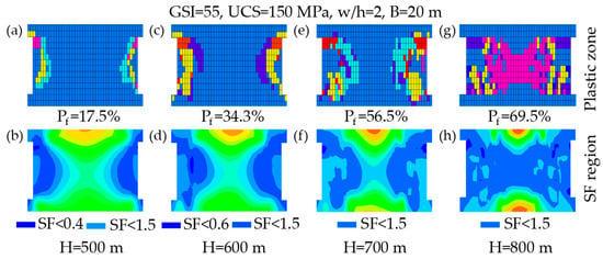
Figure 9. Impact of H on pillar stability under constant rock mass quality (GSI = 55).

Finally, the stabilizing effect of rock mass quality was highlighted under a challenging deep condition (H = 700 m, UCS = 150 MPa, w/h = 2, B = 20 m). As shown in Figure 10a,b, the pillar exhibited 337 plastic zone elements and P_f = 84.3% under GSI = 25, and the SF < 1.5 region spread across nearly the entire pillar, matching an “X-shaped” connected plastic zone and indicating failure. For GSI = 55, plastic zone decreased to 226 elements with P_f = 56.5% (see Figure 10c). As illustrated in Figure 10d, the plastic zone and SF < 1.5 region remained extensive but did not fully connect, indicating high instability probability without complete failure. In contrast, the plastic zone elements dropped to 56 and P_f = 14.0% under GSI = 85 (see Figure 10e), and it can be seen that from Figure 10f that the SF < 1.5 region was localized and consistent with a limited plastic zone, suggesting a stable pillar even at the same depth.

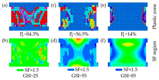
Figure 10. Impact of GSI on pillar stability for fixed operating conditions (H = 700 m, UCS = 150 MPa, w/h = 2, B = 20 m).

4.2. AI Prediction

4.2.1. Model Development and Optimization

In this study, six ML models were developed using a database consisting 100 samples collected from numerical simulations to predict P_f of legacy pillars. To improve predictive accuracy, the CCO optimization algorithm was employed to determine the optimal hyperparameters for each model. The search ranges of the hyperparameters are listed in Table 1. Figure 11 illustrates the iterative convergence curves of the optimized models under different population sizes (30, 60, 90, and 120). It can be observed that all optimized models identified their optimal hyperparameter combinations before reaching the maximum number of iterations, as indicated by stable minimum values in the convergence curves. Table 2 records the minimum fitness values of each optimized model under different population sizes. The results show that all models achieved their best hyperparameter combinations when population size equal 90.

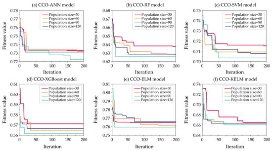
Figure 11. Iteration curves of hybrid ML models optimized by CCO under different population sizes.

Table 2. Fitness values of all ML models optimized by CCO algorithm with different population sizes.

Models	Population Sizes				Hyperparameters
	30	60	90	120
CCO-ANN	0.7329	0.7317	0.7224	0.7311	Nh = 1; Nn = 6
CCO-RF	0.6377	0.6281	0.6257	0.6286	Nt = 55; Minleaf = 1
CCO-SVM	0.7154	0.7094	0.7035	0.7079	C = 5.13; kp = 0.56
CCO-XGBoost	0.5711	0.5642	0.5617	0.5665	Ne = 65; Lr = 0.25; Maxdepth = 5
CCO-ELM	0.7649	0.7611	0.7594	0.7658	Nn = 105
CCOKELM	0.6650	0.6636	0.6604	0.6634	C = 12.56; kp = 0.712

After determining the optimal hyperparameter combinations of all models, their prediction accuracy needs to be evaluated using test set. Four statistical indicators were first employed to compare the performance of the models on the test dataset, and the corresponding values are reported in Table 3. For the R² and VAF metrics, higher values indicate better predictive accuracy. In contrast, lower RMSE and MAE values imply smaller prediction errors and thus superior model performance. As shown in the table, the CCO-XGBoost model achieves the highest R² and VAF values (0.9036 and 93.1193%), as well as the lowest RMSE and MAE values (4.4904 and 3.9539). The RF and KELM models also outperform the remaining models in terms of these indicators. Based on the evaluation criteria, the models were ranked and assigned scores accordingly. For example, the top-ranked model received 6 points, whereas the lowest-ranked model received only 1 point. The resulting overall performance ranking of the models is as follows: CCO-XGBoost > CCO-RF > CCO-SVM (CCO-KELM) > CCO-ANN > CCO-ELM models.

Table 3. Performance evaluation using four statistical indicators for all developed models.

Models	Evaluation Indicators				Ranking
	R2	RMSE	VAF (%)	MAE
CCO-ANN	0.8194	6.1454	82.4893	4.1386	10
CCO-RF	0.8815	4.9782	91.5206	4.4194	18
CCO-SVM	0.8394	5.7954	83.9755	4.1199	14
CCO-XGBoost	0.9036	4.4904	93.1193	3.9539	24
CCO-ELM	0.7850	6.7055	81.5216	5.7518	4
CCOKELM	0.8672	5.2698	90.0707	4.5454	14

Furthermore, regression plots were used to evaluate model performance. In a regression plot, the position of each data point is determined by its predicted and actual values. Under perfect prediction, the predicted values equal the actual values, and all points lie on the diagonal line. As prediction errors increase, data points deviate further from the diagonal. However, achieving perfect prediction is challenging, and small errors are generally acceptable in practical regression tasks. Therefore, a 5% error tolerance band was defined in this study to assess model performance. Data points located outside the tolerance band were regarded as outliers, and a larger number of outliers (NO) indicates poorer model performance. Figure 12 illustrates the data distributions of the predictions for each model along with the corresponding NO values. It can be observed that the CCO-XGBoost model yields the lowest NO value (5), whereas the CCO-ELM model produces 14 outliers due to its inferior predictive performance. However, boxplot comparisons of the predicted and actual value distributions reveal that, although CCO-XGBoost achieves fewer outliers, the prediction distribution (minimum, mean, and maximum: 46.6, 70.2, and 96.2%) of the CCO-SVM model is closer to the actual value distribution (minimum, mean, and maximum: 47, 70.5, and 95%).

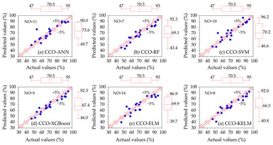
Figure 12. Regression graphs of all hybrid ML models based on the test set.

Moreover, Figure 13 compares the prediction error characteristics of the COO-SVM and COO-XGBoost models across all samples using cumulative error, error dispersion, and the integrated error curve. Although the two models exhibit comparable area under the error curve (AUC) values (74.40 for COO-SVM and 74.29 for COO-XGBoost), their error accumulation patterns and stability differ noticeably. COO-XGBoost yields a smaller total error sum (Sum: 79.07) and a markedly lower standard deviation (St. D: 2.18) than COO-SVM, indicating a more consistent error distribution across different samples. In contrast, COO-SVM shows a larger error dispersion (St. D = 4.18). The error curves further reveal that COO-XGBoost maintains a smoother and more gradual error decay, whereas COO-SVM exhibits steeper variations at early samples. These results indicate that while both models achieve comparable overall integrated performance, COO-XGBoost provides superior robustness and reliability.

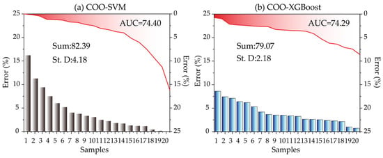
Figure 13. Performance comparison between COO-SVM and COO-XGBoost models.

4.2.2. Model Interpretability

Although the optimal prediction has been determined after model evaluation, the influence of all input features on P_f prediction was unknown. As shown in Figure 14a, the feature importance scores indicate that H has the highest influence on the predicted pillar instability probability, followed by pillar w/h, UCS, GSI, and B. The SHAP-based contribution analysis further reveals the directional effects of these parameters (see Figure 14b). Increasing H produces predominantly positive SHAP values, confirming that higher in situ stress systematically elevates instability risk. The contribution of w/h shows a clear sign change: smaller ratios contribute positively to instability, while larger ratios yield negative contributions, reflecting the enhanced load-bearing capacity of wider pillars. UCS mainly exhibits negative SHAP values when increased, indicating a stabilizing effect, although the contribution magnitude varies with operating conditions. Notably, despite its lower global importance score, GSI displays a coherent and systematic contribution pattern, highlighting its role as a critical modifier of instability rather than a primary driver. Higher GSI values are predominantly associated with negative contributions, implying reduced instability probability through improved rock mass integrity and surface condition of the pillar. B shows the lowest importance score, with SHAP values clustered near zero, implying a limited and condition-dependent influence. Overall, the stress level and pillar geometry govern stability, material strength provides secondary support, and span effects become significant only under specific configurations.

Figure 14. Interpretability of the optimal model through SHAP analysis.

4.2.3. Case Study

A legacy pillar located in the S9–10# experimental stope at a depth of −550 m in the Fankou lead–zinc mine was selected as a representative case to verify the proposed framework. The geometric and mechanical properties of the pillar are as follows: width of 6 m, height of 3 m, density of 3460 kg/m³, and UCS of 125 MPa. To determine the rock mass quality of the pillar, the GSI was evaluated using the 3D Geological Structure Measurement (3GSM) system. The system employs a wearable high-resolution camera to capture detailed geometric information of discontinuities, including orientation, trace length, spacing, and persistence. The collected discontinuity data were processed by the internal software to perform classification, grouping, and statistical analysis of geometric parameters. Based on the processed structural information and standard GSI charts and calculation procedures, the GSI value of the pillar was estimated to be 60. Using the above parameters, a numerical model was established with appropriate boundary conditions and excavation sequences to simulate the mechanical behavior of the pillar. The resulting pillar stability is illustrated in Figure 15. As shown in Figure 15a, a total of 80 pillar elements entered a yielding state. According to Equation (1), the corresponding P_f was calculated as 20%. The plastic zones initiate at both lateral sides of the pillar and progressively propagate toward the central region, indicating that instability is expected once the yielding zones from both sides become fully connected. Figure 15b shows that regions with a SF lower than 1.5 are spatially consistent with the distribution of plastic zones, further confirming the reliability of the adopted instability criterion.

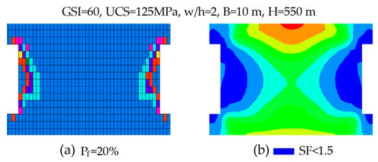
Figure 15. Numerical simulation of pillar stability for a case study.

In addition, to evaluate the predictive performance of the proposed framework under typical variability and uncertainty of field measurements, a reliability analysis was conducted for the input parameters based on previous investigations in experimental mining sites. The statistical characteristics of the input variables are summarized in Table 4. Using the Monte Carlo method, 1000 random realizations were generated and subsequently input into the established model. The resulting average pillar instability probability was 19.393%, which is in close agreement with the numerically obtained P_f value of 20%. This consistency indicates that the proposed framework maintains stable predictive capability under realistic parameter variability and demonstrates its effectiveness for practical assessment of legacy pillar instability.

Table 4. Statistical results of parameters for the case pillar.

Statistical Indices	GSI	UCS (MPa)	w/h	B (m)
Maximum	63	150	2.2	12
Minimum	57	130	1.2	9
Mean	60	135	1.7	10.5
Standard deviation	2.5	9.6	0.9	1.1
Coefficient of variation	0.05	0.2	0.08	0.13

5. Conclusions

This study developed an integrated numerical simulation and AI framework to assess the instability probability of legacy pillars. The approach combined physics-based simulation with ML-based probabilistic prediction and using metaheuristic optimization to improve model performance. The main conclusions can be summarized as follows:

(1) Numerical simulation results showed that pillar instability probability was primarily controlled by B, H, w/h, UCS, and GSI. Increasing H significantly increased instability probability due to elevated in situ stress, while larger w/h and higher UCS enhanced pillar stability. Although GSI did not dominate the response, it consistently influenced failure development and instability probability by modifying stress redistribution and plastic zone evolution.

(2) Among the developed ML models, the CCO-XGBoost model achieved the most balanced performance in terms of accuracy, robustness, and error stability for predicting P_f, with the highest R² and VAF values (0.9036 and 93.1193%), as well as the lowest RMSE and MAE values (4.4904 and 3.9539).

(3) Feature importance and SHAP-based contribution analyses confirmed the physical consistency of the proposed framework. H was identified as the most influential parameter, followed by w/h and UCS, while GSI acted as a critical modifier that differentiated instability probability under similar stress and geometric conditions.

(4) The predicted P_f offers a practical basis for screening and prioritizing legacy pillars with elevated risk levels, rather than defining universal alarm thresholds, thereby supporting engineering decisions related to inspection frequency, monitoring deployment, and mitigation planning.

In the present study, the machine learning models are trained using data derived from numerical simulations and are therefore intended as surrogate predictors rather than direct field-calibrated models. Although this framework enables efficient probabilistic assessment while maintaining physical consistency, it does not explicitly incorporate measurement noise or site-specific variability typically observed in field conditions. Furthermore, the framework evaluates pillar instability under instantaneous or quasi-static conditions and does not explicitly account for time-dependent geomechanical processes. In long-term scenarios such as mine closure, pillar stability may be influenced by progressive degradation mechanisms, including creep deformation, damage accumulation, stress redistribution, and environmental effects. The proposed methodology is therefore best suited for snapshot stability assessment based on current conditions. In addition, buckling-related geometric instability is not explicitly considered. As a result, the applicability of the framework is limited to short and moderately slender pillars, for which failure is dominated by material yielding and stress redistribution rather than global geometric instability. Extension of the framework to time-dependent or buckling-dominated failure modes would require enhanced constitutive descriptions or geometric considerations within the numerical modeling component.

References

- Prior, T.; Giurco, D.; Mudd, G.; Mason, L.; Behrisch, J. Resource depletion, peak minerals and the implications for sustainable resource management. Glob. Environ. Change 2012, 22, 577–587. [Google Scholar] [CrossRef]
- Dong, L.; Tong, X.; Li, X.; Zhou, J.; Wang, S.; Liu, B. Some developments and new insights of environmental problems and deep mining strategy for cleaner production in mines. J. Clean. Prod. 2019, 210, 1562–1578. [Google Scholar] [CrossRef]
- Yang, Z. Key technology research on the efficient exploitation and comprehensive utilization of resources in the deep Jinchuan nickel deposit. Engineering 2017, 3, 559–566. [Google Scholar] [CrossRef]
- Ranjan, A.; Zhao, Y.; Sahu, H.B.; Misra, P. Opportunities and challenges in health sensing for extreme industrial environment: Perspectives from underground mines. IEEE Access 2019, 7, 139181–139195. [Google Scholar] [CrossRef]
- Li, C.; Zhou, J.; Armaghani, D.J.; Li, X. Stability analysis of underground mine hard rock pillars via combination of finite difference methods, neural networks, and Monte Carlo simulation techniques. Undergr. Space 2021, 6, 379–395. [Google Scholar] [CrossRef]
- Zvarivadza, T.; Grobler, H.; Olubambi, P.A.; Onifade, M.; Khandelwal, M. Hybrid pillar stress analysis: Integrating numerical modelling, machine learning, and geostatistics for improved stability in hardrock mining. Results Earth Sci. 2025, 3, 100129. [Google Scholar] [CrossRef]
- Ghasemi, E.; Shahriar, K. A new coal pillars design method in order to enhance safety of the retreat mining in room and pillar mines. Saf. Sci. 2012, 50, 579–585. [Google Scholar] [CrossRef]
- Hustrulid, W.A. A review of coal pillar strength formulas. Rock Mech. 1976, 8, 115–145. [Google Scholar]
- Salamon, M.D.G.; Munro, A. A study of the strength of coal pillars. J. S. Afr. Inst. Min. Metall. 1967, 68, 55–67. [Google Scholar]
- Van der Merwe, J.N. New pillar strength formula for South African coal. J. S. Afr. Inst. Min. Metall. 2003, 103, 281–292. [Google Scholar]
- Prassetyo, S.H.; Irnawan, M.A.; Simangunsong, G.M.; Wattimena, R.K.; Arif, I.; Rai, M.A. New coal pillar strength formulae considering the effect of interface friction. Int. J. Rock Mech. Min. Sci. 2019, 123, 104102. [Google Scholar] [CrossRef]
- Hedley, D.G.F.; Grant, F. Stope-and-pillar design for the Elliot Lake Uranium Mines. Bull. Can. Inst. Min. Met. 1972, 65, 37–44. [Google Scholar]
- Watson, B.P.; Ryder, J.A.; Kataka, M.O.; Kuijpers, J.S.; Leteane, F.P. Merensky pillar strength formulae based on back-analysis of pillar failures at Impala Platinum. J. S. Afr. Inst. Min. Metall. 2008, 108, 449–461. [Google Scholar]
- González-Nicieza, C.; Álvarez-Fernández, M.I.; Menéndez-Díaz, A.; Alvarez-Vigil, A.E. A comparative analysis of pillar design methods and its application to marble mines. Rock Mech. Rock Eng. 2006, 39, 421–444. [Google Scholar] [CrossRef]
- Esterhuizen, G.S.; Dolinar, D.R.; Ellenberger, J.L. Pillar strength in underground stone mines in the United States. Int. J. Rock Mech. Min. Sci. 2011, 48, 42–50. [Google Scholar] [CrossRef]
- Li, W.; Bai, J.; Peng, S.; Wang, X.; Xu, Y. Numerical modeling for yield pillar design: A case study. Rock Mech. Rock Eng. 2015, 48, 305–318. [Google Scholar] [CrossRef]
- Kortnik, J. Stability assessment of the high safety pillars in Slovenian natural stone mines. Arch. Min. Sci. 2015, 60, 403–417. [Google Scholar] [CrossRef]
- Wang, S.Y.; Lam, K.C.; Au, S.K.; Tang, C.A.; Zhu, W.C.; Yang, T.H. Analytical and numerical study on the pillar rockbursts mechanism. Rock Mech. Rock Eng. 2006, 39, 445–467. [Google Scholar] [CrossRef]
- Chen, T.; Mitri, H.S. Strategies for surface crown pillar design using numerical modelling—A case study. Int. J. Rock Mech. Min. Sci. 2021, 138, 104599. [Google Scholar] [CrossRef]
- Zheng, H.; Li, P.; Ma, G. Stability analysis of the middle soil pillar for asymmetric parallel tunnels by using model testing and numerical simulations. Tunn. Undergr. Space Technol. 2021, 108, 103686. [Google Scholar] [CrossRef]
- Mortazavi, A.; Hassani, F.P.; Shabani, M. A numerical investigation of rock pillar failure mechanism in underground openings. Comput. Geotech. 2009, 36, 691–697. [Google Scholar] [CrossRef]
- Renani, H.R.; Martin, C.D. Modeling the progressive failure of hard rock pillars. Tunn. Undergr. Space Technol. 2018, 74, 71–81. [Google Scholar] [CrossRef]
- Kim, J.G.; Abdellah, W.R.; Yang, H.S. Parametric stability analysis of pillar performance at Nohyun limestone mine, South Korea—A case study. Arab. J. Geosci. 2019, 12, 390. [Google Scholar] [CrossRef]
- Kumar, A.; Waclawik, P.; Singh, R.; Ram, S.; Korbel, J. Performance of a coal pillar at deeper cover: Field and simulation studies. Int. J. Rock Mech. Min. Sci. 2019, 113, 322–332. [Google Scholar] [CrossRef]
- Tawadrous, A.S.; Katsabanis, P.D. Prediction of surface crown pillar stability using artificial neural networks. Int. J. Numer. Anal. Methods Geomech. 2007, 31, 917–931. [Google Scholar] [CrossRef]
- Kumar, M.; Avchar, A.; Sinha, S.; Swamy, S.V. Integrated approaches for pillar design and stability assessment in underground hard rock mining: From empirical models to machine learning. Phys. Chem. Earth Parts A/B/C 2025, 142, 104235. [Google Scholar] [CrossRef]
- Li, C.; Zhou, J.; Du, K.; Dias, D. Stability prediction of hard rock pillar using support vector machine optimized by three metaheuristic algorithms. Int. J. Min. Sci. Technol. 2023, 33, 1019–1036. [Google Scholar] [CrossRef]
- Kamran, M.; Chaudhry, W.; Taiwo, B.O.; Hosseini, S.; Rehman, H. Decision intelligence-based predictive modelling of hard rock pillar stability using K-nearest neighbour coupled with grey wolf optimization algorithm. Processes 2024, 12, 783. [Google Scholar] [CrossRef]
- Alhamrouni, I.; Abdul Kahar, N.H.; Salem, M.; Swadi, M.; Zahroui, Y.; Kadhim, D.J.; Mohamed, F.A.; Alhuyi Nazari, M. A comprehensive review on the role of artificial intelligence in power system stability, control, and protection: Insights and future directions. Appl. Sci. 2024, 14, 6214. [Google Scholar] [CrossRef]
- Ghasemi, E.; Kalhori, H.; Bagherpour, R. Stability assessment of hard rock pillars using two intelligent classification techniques: A comparative study. Tunn. Undergr. Space Technol. 2017, 68, 32–37. [Google Scholar] [CrossRef]
- Idris, M.A.; Saiang, D.; Nordlund, E. Stochastic assessment of pillar stability at Laisvall mine using artificial neural network. Tunn. Undergr. Space Technol. 2015, 49, 307–319. [Google Scholar] [CrossRef]
- Ding, H.; Li, G.; Dong, X.; Lin, Y. Prediction of pillar stability for underground mines using the stochastic gradient boosting technique. IEEE Access 2018, 6, 69253–69264. [Google Scholar] [CrossRef]
- Zhou, J.; Li, X.-B.; Shi, X.-Z.; Wei, W.; Wu, B.-B. Predicting pillar stability for underground mine using Fisher discriminant analysis and SVM methods. Trans. Nonferrous Met. Soc. China 2011, 21, 2734–2743. [Google Scholar] [CrossRef]
- Zhou, J.; Li, X.; Mitri, H.S. Comparative performance of six supervised learning methods for the development of models of hard rock pillar stability prediction. Nat. Hazards 2015, 79, 291–316. [Google Scholar] [CrossRef]
- Qiu, Y.; Zhou, J. Methodology for constructing explicit stability formulas for hard rock pillars: Integrating data-driven approaches and interpretability techniques. Rock Mech. Rock Eng. 2025, 58, 5475–5502. [Google Scholar] [CrossRef]
- Li, N.; Zare, M.; Yi, C.; Jimenez, R. Stability risk assessment of underground rock pillars using logistic model trees. Int. J. Environ. Res. Public Health 2022, 19, 2136. [Google Scholar] [PubMed]
- Li, C.; Zhou, J.; Armaghani, D.J.; Cao, W.; Yagiz, S. Stochastic assessment of hard rock pillar stability based on the geological strength index system. Geomech. Geophys. Geo-Energy Geo-Resour. 2021, 7, 47. [Google Scholar] [CrossRef]
- Wattimena, R.K.; Kramadibrata, S.; Sidi, I.D.; Azizi, M.A. Developing coal pillar stability chart using logistic regression. Int. J. Rock Mech. Min. Sci. 2013, 58, 55–60. [Google Scholar] [CrossRef]
- Wattimena, R.K. Predicting the stability of hard rock pillars using multinomial logistic regression. Int. J. Rock Mech. Min. Sci. 2014, 71, 33–40. [Google Scholar] [CrossRef]
- Soltani, A. Analysis of the ARMPS Database Using FLAC3d; A Pillar Stability Comparison for Room and Pillar Coal Mines During Development. Master’s Thesis, University of Kentucky, Lexington, KY, USA, 2015. Available online: https://uknowledge.uky.edu/mng_etds/22 (accessed on 20 December 2025).
- Abiodun, O.I.; Jantan, A.; Omolara, A.E.; Dada, K.V.; Mohamed, N.A.; Arshad, H. State-of-the-art in artificial neural network applications: A survey. Heliyon 2018, 4, e00938. [Google Scholar] [CrossRef] [PubMed]
- Salman, H.A.; Kalakech, A.; Steiti, A. Random forest algorithm overview. Babylon. J. Mach. Learn. 2024, 2024, 69–79. [Google Scholar] [CrossRef] [PubMed]
- Xu, Y. A rough margin-based linear ν support vector regression. Stat. Probab. Lett. 2012, 82, 528–534. [Google Scholar]
- Zhou, J.; Qiu, Y.; Zhu, S.; Armaghani, D.J.; Khandelwal, M.; Mohamad, E.T. Estimation of the TBM advance rate under hard rock conditions using XGBoost and Bayesian optimization. Undergr. Space 2021, 6, 506–515. [Google Scholar] [CrossRef]
- Li, C.; Zhou, J.; Khandelwal, M.; Zhang, X.; Monjezi, M.; Qiu, Y. Six novel hybrid extreme learning machine–swarm intelligence optimization (ELM–SIO) models for predicting backbreak in open-pit blasting. Nat. Resour. Res. 2022, 31, 3017–3039. [Google Scholar] [CrossRef]
- Li, E.; Zhang, N.; Xi, B.; Yu, Z.; Fissha, Y.; Taiwo, B.O.; Segarra, P.; Feng, H.; Zhou, J. Analysis and modelling of gas relative permeability in reservoir by hybrid KELM methods. Earth Sci. Inform. 2024, 17, 3163–3190. [Google Scholar] [CrossRef]
- Wang, T.L.; Gu, S.W.; Liu, R.J.; Chen, L.Q.; Wang, Z.; Zeng, Z.Q. Cuckoo catfish optimizer: A new meta-heuristic optimization algorithm. Artif. Intell. Rev. 2025, 58, 326. [Google Scholar] [CrossRef]
- Yang, X.S. Swarm intelligence based algorithms: A critical analysis. Evol. Intell. 2014, 7, 17–28. [Google Scholar] [CrossRef]
- Chakraborty, A.; Kar, A.K. Swarm intelligence: A review of algorithms. In Nature-Inspired Computing and Optimization; Springer: Cham, Switzerland, 2017; pp. 475–494. [Google Scholar]
- Veeranjaneyulu, K.; Lakshmi, M.; Janakiraman, S. Swarm intelligent metaheuristic optimization algorithms-based artificial neural network models for breast cancer diagnosis: Emerging trends, challenges and future research directions. Arch. Comput. Methods Eng. 2025, 32, 381–398. [Google Scholar] [CrossRef]
Disclaimer/Publisher’s Note: The statements, opinions and data contained in all publications are solely those of the individual author(s) and contributor(s) and not of MDPI and/or the editor(s). MDPI and/or the editor(s) disclaim responsibility for any injury to people or property resulting from any ideas, methods, instructions or products referred to in the content. |
© 2026 by the authors. Licensee MDPI, Basel, Switzerland. This article is an open access article distributed under the terms and conditions of the Creative Commons Attribution (CC BY) license.