A Novel Linguistic Framework for Dynamic Multi-Criteria Group Decision-Making Using Hedge Algebras

Abstract

Dynamic multi-criteria group decision-making (MCGDM) is widely applied in complex real-world settings where multiple experts evaluate alternatives across diverse criteria under uncertain and evolving conditions. This study proposes a transparent and interpretable linguistic (L-) framework for dynamic MCGDM grounded in hedge algebras (HA), a mathematical formalism that provides explicit algebraic and semantic structures for L-domains. A novel binary L-aggregation operator is developed using the 4-tuple semantic representation of HA, ensuring closure, commutativity, monotonicity, partial associativity, the existence of an identity element, and semantic consistency throughout the aggregation process. Using this operator, a two-stage dynamic decision-making model is developed—(i) L-FAHP for determining the criterion weights in dynamic environments, and (ii) L-FTOPSIS for ranking alternatives—where both methods are formulated on HA L-scales. To address temporal dynamics, a dynamic L-aggregation mechanism is further proposed to integrate current expert judgments with historical evaluations through a semantic decay factor, enabling the controlled attenuation of outdated information. A case study on enterprise digital transformation readiness illustrates that the proposed framework enhances semantic interpretability, maintains stability under uncertainty, and more accurately captures the temporal evolution of expert assessments. These results underscore the practical value and applicability of the HA-based dynamic L-approach in complex decision environments where expert knowledge and temporal variability are critical.

1. Introduction

Multi-criteria group decision-making (MCGDM) plays a crucial role in numerous socio-economic domains, such as supplier selection [1], healthcare [2,3], transportation planning [4], education management [5], digital transformation [6,7,8,9,10,11,12,13,14,15], and risk assessment [16]. In these contexts, experts must provide judgments based on multiple criteria, and such evaluations are inherently subjective. Therefore, constructing an appropriate group decision-making model is essential to ensure the reliability of the final ranking results. A general MCGDM problem requires addressing the following issues simultaneously: (i) designing a suitable L-scale for expert evaluations; (ii) determining the weights of the criteria; (iii) assessing and ranking the alternatives with respect to each criterion; and (iv) aggregating the opinions of multiple experts to reach a conclusion.

In recent decades, fuzzy multi-criteria decision-making has emerged as one of the fastest-growing research areas [17,18,19,20,21,22,23,24,25,26,27,28,29,30,31], as it aligns well with human reasoning and perception. In practice, experts often prefer expressing their opinions using L-words rather than precise numerical values, because L-expressions better capture human cognition in uncertain and vague environments. Approaches for fuzzy group decision-making have been developed primarily based on fuzzy set theory and its extensions. One of the key challenges in solving fuzzy MCGDM problems is constructing a suitable L-information representation that experts can use to express their assessments. Several commonly used fuzzy L-representation models include 2-tuple [16,17,18,19,20], and L-modeling frameworks based on fuzzy logic tools such as fuzzy numbers [21,22], intuitionistic fuzzy sets [23], hesitant fuzzy sets [24,25], Pythagorean fuzzy sets [26,27], interval-valued neutrosophic sets [5], T-spherical fuzzy sets [28], and 4-tuple models [29,30,31], HA [31]. However, selecting and employing an appropriate fuzzy representation model remains challenging. For example, there is often a lack of a clear mathematical foundation that enables experts to formally construct fuzzy sets corresponding to L-words. Most existing approaches rely on ad hoc fuzzy membership functions and lack a rigorous mechanism to derive quantitative semantics from the inherent qualitative meanings of L-words. In many existing studies [1,3,4,5,6,21,22,24,25,26,27,28,32,33], L-scales are built upon discrete fuzzy values without formal linkage to their intrinsic semantics. This makes it difficult to define meaningful aggregation operators on the L-domain, especially in dynamic MCGDM environments [32,34,35,36,37,38] where evaluation information evolves over time and must be integrated with historical data: for example, evaluating suppliers and assessing the digital transformation level of enterprises.

HA theory was first introduced by Ho et al. [39], and it has since been further developed in subsequent studies [29,30,31,40,41,42,43]. It provides a mathematical framework that enables the mapping of L-variable domains from qualitative semantics to quantitative numerical domains. This theory establishes a rigorous formal mechanism for deriving quantitative semantics from the inherent qualitative meanings of L-words through an algebraic structure. HA has been successfully applied in various research areas, including fuzzy control [41], fuzzy regression [42], fuzzy time series forecasting [43], and MCGDM [29,30,31]. The HA approach for MCGDM provides an algebraically structured and semantically well-founded framework for constructing L-scales. Representing L-words using the 4-tuple semantic model preserves their inherent ordinal semantics throughout the computation process. A weighted-mean L-aggregation operator was introduced in [29] and applied in [30,31]. However, this aggregation does not fully reflect the semantic interactions embedded in L-words. In this study, HA is used not to introduce additional fuzziness but to provide a rigorous semantic basis for linguistic terms: something that conventional fuzzy AHP/TOPSIS cannot guarantee. By deriving quantitative meanings through an algebraic structure rather than heuristic fuzzy numbers, the HA 4-tuple model preserves ordinal semantics, hedge effects, and temporal consistency in dynamic MCGDM settings. Thus, HA enhances semantic interpretability and robustness while complementing, rather than duplicating, fuzzy logic.

By examining the behavior of real number addition—where the sum of two positive numbers is greater than each of them, the sum of two negative numbers is smaller than each, and the sum of a positive and a negative number falls between them—we draw inspiration for enhancing L-aggregation. Building on this property of the real number domain and the structure used to generate L-words in HA, we propose a binary L-aggregation operator for 4-tuple L-words. This is accompanied by a procedure for constructing the triangular fuzzy semantics of L-words within the L-Frame of Cognitive, as described in [42]. The proposed operator is then applied to address a dynamic MCGDM problem.

In this paper, we present a novel L-framework for dynamic MCGDM, based on HA. The main contributions are as follows:

(i) A new binary L-aggregation operator for 4-tuple semantic representations that ensures closure, commutativity, monotonicity, partial associativity, and the existence of an identity element on the L-scale, L_k.

(ii) A two-phase framework for solving dynamic MCGDM using HA-based L-scales:

Phase 1: Development of an L-FAHP for determining criterion weights in a dynamic environment.

Phase 2: Development of an L-FTOPSIS for ranking alternatives in a dynamic environment.

(iii) A dynamic L-aggregation mechanism that integrates current expert assessments with historical information through a semantic decay parameter.

(iv) An empirical case study demonstrates the practical applicability of the proposed framework by addressing the issue of ranking enterprise digital transformation readiness, which is a problem of significant relevance within the national digital transformation program.

Digital transformation has become indispensable for the survival and long-term development of contemporary enterprises because it enhances operational efficiency, strengthens forecasting capability, optimizes costs, and improves competitive advantage. The existing research consistently indicates that organizations which delay digital transformation face an increased risk of being displaced in an environment characterized by intensifying competition [44]. Digital transformation should not be understood solely as the adoption of new technologies, but rather as a comprehensive restructuring of business models, value chains, operational processes, data systems, and organizational structures, while at the same time creating superior customer experiences. This requirement has become even more pronounced as consumer behavior continues to undergo profound changes [45]. Evaluating digital maturity plays a crucial role in enabling enterprises to understand their current position, determine priority areas for investment, allocate limited resources effectively, and mitigate risks during the implementation of digital initiatives. This evaluation is particularly important for small and medium-sized enterprises, which often lack technological capacity and practical experience in digital transformation [46]. In the retail sector, where digital transformation exerts an especially strong influence due to the rapid expansion of e-commerce, rising expectations for personalization, and the development of omnichannel business models, digital transformation has emerged as a prerequisite for maintaining competitiveness, optimizing operational activities, managing inventory and logistics, and improving customer experience [45]. Overall, digital transformation and the assessment of digital maturity constitute the foundation for sustainable development strategies for enterprises in general, and for retail businesses, particularly in the digital era. The complexity of digital transformation in retail enterprises requires the simultaneous evaluation of multiple dimensions, including technological capability, organizational readiness, data maturity, customer experience, process integration, and business model innovation. Consequently, the assessment of digital maturity can be considered a MCGDM process in which various dimensions must be analyzed concurrently to ensure a comprehensive and accurate evaluation [45,46].

The remainder of the paper is organized as follows: Section 2 presents the fundamental concepts of HA and the 4-tuple L-representation. Section 3 introduces the L-framework for dynamic MCGDM, based on L-FAHP and L-FTOPSIS. Section 4 illustrates the applicability of the proposed framework through a case study assessing the digital transformation readiness of enterprises in Vietnam. A comparative analysis is provided in Section 5. Sensitivity analysis and the discussion are presented in Section 6. Finally, Section 7 concludes the paper and outlines directions for future research.

2. Preliminary

2.1. The Concepts of the HAs

In human society, people utilize their historical experiences to communicate with one another through words in their natural language. The L-words themselves reveal their inherent semantics. Because these semantics are qualitative, every word possesses a semantic order relation with each of the other words within the word-domain of an L-variable. Consequently, any mathematical theory developed to model the semantics of words belonging to a variable must be able to handle this semantic structure; for instance, it must preserve the order-based structure of the word-domain. It can be easily observed that fuzzy set theory does not preserve these order-based structures. Each L-domain of a variable X, denoted by Dom(X), consists of a set of words that can be generated from two generator words, e.g., “unimportant” and “important”, by the action of L-hedges on them. For example, with two hedges such as “very” and “little” acting on the two generator words “important” and “unimportant”, the generated words can be “very unimportant”, “little unimportant”, “little important”, “very important”, and so on. It can be observed that they are linearly ordered and comparable, e.g., “very unimportant” ≤ “unimportant” ≤ “little unimportant” ≤ “little important” ≤ “important” ≤ “very important”.

That motivated Ho et al. [39] to introduce HA, a mathematical structure that can directly manipulate the word domain of X. HA has been developed in numerous studies [29,30,31,40,41,42,43]. The HA theory has introduced many semantic aspects of L-words and supports computing with words in applications, such as fuzziness measures, quantitative values or numeric semantics, similarity intervals, fuzzy set semantics, and 4-tuple semantic representations, which facilitate the synthesis of L-words in group decision-making problems.

Definition 1. 

An HA of an L-variable X is defined in [39], as follows:

AX = (X, G, C, H, σ, Φ, ≤),

where

• X is a set of words and X ⊆ Dom(X).
• G ={$c^{-}$, $c^{+}$} is a set of two generators, in which $c^{-} \le { c}^{+}$; for instance, unimportant$\le$important.
• C = {0, w, 1} is the set of three constants interpreted as the smallest, the neutral, and the largest word in X, satisfying the ordering 0 <$c^{-}$< w < $c^{+}$ < 1; for example, these constants correspond to the specific words “extremely unimportant”$\le$“unimportant”$\le$“medium”$\le$“important”$\le$“extremely important”.
• H = $H^{-}$ $\cup$ $H^{+}$, where $H^{-}$and $H^{+}$are the sets of negative and positive hedges such as “very” and “little”.
• σ and Φ are specific artificial operators that determine the supremum and infimum, respectively, of a subset of the word domain X.
• ≤ is a semantic ordering relation defined on X.

Each L-value in HA has its own semantics. To quantitatively model the semantics of all L-words within a word-domain, two fundamental notions of HA must be established: the semantically quantifying mapping (SQM) and the fuzziness measure $\left(fm\right)$ are denoted as $\vartheta$: X → [0, 1] and $fm$: X → [0, 1], respectively. These two constructs formally define how L-words are quantitatively represented and how their inherent fuzziness is measured within the HA structure, as follows:

Definition 2

([40]).

Let AX = (X, G, C, H, σ, Φ, ≤) be a linear complete HA (ComHA) of a given L-variable Y. A mapping $fm$: X → [0, 1] is called a fuzzy measure of words in X, provided that

(i) $fm$(c⁻) + $fm$(c⁺) = 1;

(ii) ∑_h∈H $fm$(hu) = $fm$(u), ∀u ∈ X;

(iii) $fm$(0) = $fm$(w) = $fm$(1) = 0, and the fm of all constants is 0;

(iv) ∀x, y ∈ X, ∀h ∈ H, the ratio $\mu \left(h\right)={\displaystyle \frac{fm\left(hx\right)}{fm\left(x\right)}}={\displaystyle \frac{fm\left(hy\right)}{fm\left(y\right)}}$, is independent of x and y, and is referred to as the fuzzy measure of the hedge h, denoted by$\mu \left(h\right)$.

The main properties of the fm for words and hedges are as follows:

(i) $fm$(c⁻) + $fm$(c⁺) = 1;

(ii) $\sum _{j=-q}^{-1}\mu \left(h_j\right)=\alpha$, $\sum _{j=1}^p\mu \left(h_j\right)=\beta$, where α, β > 0 and α + β = 1;

(iii) $\sum _{-q \le i \le p, j \ne 0 }fm( h_{j}x)=fm \left(x\right)$, $\forall x\in$ X;

(iv) fm(hx) = μ(h)fm(x), $\forall x\in$ X.

Analogous to the algebraic sign of numbers in classical analysis, the algebraic signs of L-words in X are defined via a sign function, as follows:

Definition 3

([40]).

The sign function ζgη: X⟶ {−1, 0, 1} is a mapping defined recursively as follows, where h, h’∈ H and c∈ {c⁻, c⁺}:

(i) ζgη(c⁻) = −1, ζgη (c⁺) = +1;

(ii) ζgη (hc) = −ζgη (c) if hc < c, and ζgη (hc) = +ζgη (c) if hc > c;

(iii) ζgη (h’hx) = 0 if h’hx = hx; ζgη (h’hx) = −ζgη(hx), if h’hx ≠ hx and h’ is negative with respect to h; otherwise ζgη(h’hx) = ζgη(hx), if h’hx ≠ hx and h’ is positive with respect to h;

(iv) ζgη(h’hx) = 0, if h’hx = hx.

A significant concept regarding words in natural language is their numeric semantics, which we can formalize as a semantically quantifying mapping, as follows:

Definition 4

([40]).

Let AX = (X, G, C, H, σ, Φ, ≤) be a free linear ComHA and let fm be a fuzzy measure of X. A mapping ϑ: X ⟶ [0, 1] is said to be induced by fm if it is recursively defined, as follows:

(i) ϑ(w) = θ =fm(c⁻), ϑ(c⁻) = θ − αfm(c⁻) = βfm(c⁻), ϑ(c⁺) = θ +αfm(c⁺);

(ii) ϑ(h_jx) = ϑ(x) + ζg$\left(h_{j}x\right)\left\{\sum _{i = \zeta g\left(j\right)}^j\mu \left(h_i\right)fm\left(x\right)-\omega \left(h_{j}x\right)\mu \left(h_{j}x\right)fm\left(x\right)\right\}$, for all j, where –q ≤ j ≤ p, j ≠ 0, and$\omega \left(h_{j}x\right)={\displaystyle \frac{1}{2}}\left[1+\zeta g\left(h_{j}x\right)\zeta g\left(h_p{h}_{j}x\right)(\beta -\alpha )\right]$;

(iii) ϑ(Φc⁻) = 0, ϑ(σc⁻) = θ = ϑ(Φc⁺), ϑ(σc⁺) = 1, and for all j, –q ≤ j ≤ p,

ϑ(Φ$h_{j}x$) = ϑ(x)+ ζg$\left(h_{j}x\right)\left\{\sum _{i=\zeta g\left(j\right)}^{j }\mu \left(h_i\right)fm\left(x\right)\right\}-{\displaystyle \frac{1}{2}}\left(1-\zeta g\left(h_{j}x\right)\right)\mu \left(h_i\right)fm(x)$,

ϑ(σ$h_{j}x$) = ϑ(x)+ ζg$\left(h_{j}x\right)\left\{\sum _{i = \zeta g\left(j\right)}^{j }\mu \left(h_i\right)fm\left(x\right)\right\}+ {\displaystyle \frac{1}{2}}\left(1+ \zeta g\left(h_{j}x\right)\right)\mu \left(h_i\right)fm(x)$.

It can be shown that this definition satisfies the requirements of a semantic quantification function and guarantees that the resulting values are densely distributed over the interval [0, 1].

Definition 5

([40]).

Given a fuzzy measure fm on X, a value k > 0, and a finite set of words $X_{\left(k\right)}$= {x ∈ X: |x| ≤ k}, we construct a set of intervals, {$S_{\left(k\right)}\left(x\right)$: x ∈ $X_{\left(k\right)}$} on the normalized reference domain [0, 1] called k-similarity intervals, which satisfy the following conditions:

(1) They form a partition of [0, 1].

(2) Each $S_{\left(k\right)}\left(x\right)$contains exactly one value ϑ(x) from the set {ϑ(y): y ∈ $X_{\left(k\right)}$}, where ϑ is the SQM induced by fm. The values in $S_{\left(k\right)}\left(x\right)$can be considered as being similar only to υ(x) or, more expressively, as being similar to the meaning of x at degree k.

The construction of $S_{\left(k\right)}\left(x\right)$is based on utilizing the fuzziness intervals of a higher degree k’ > k (often k’ ≥ k + 2), which are partitioned into disjoint clusters C(x) corresponding to each word x; $S_{\left(k\right)}\left(x\right)$is then defined as the union of these consecutive fuzziness intervals that cluster around the word’s SQM value ϑ(x). Note that the k-similarity interval, along with the fuzziness measure, fuzziness intervals, and the SQM, is completely determined once the fuzziness parameter values (such as fm($c^{-}$) and $\mu \left(h\right)$) of the L-variable are provided.

2.2. The 4-Tuple Semantic Linguistic Scales

The 4-tuple semantic representation model was developed to address the limitations of previous computing with word approaches in fuzzy decision-making. Traditional fuzzy set-based models required L-approximation, causing information loss, while symbolic models like the 2-tuple approach failed to preserve structural semantics. Moreover, existing models did not capture the inherent qualitative, order-based semantics of L-words. The 4-tuple model in [30] generalizes the 2-tuple approach by formally linking qualitative semantics, represented by HA, with quantitative semantics to ensure semantic soundness and computational robustness.

Definition 6

([30]).

The 4-tuple semantic representation for an L-variable and its normalized numeric reference domain is defined in the following form:

$$(x, S_{\left(k\right)}\left(x\right), \mathsf{\vartheta }\left(x\right),{ r}_x)$$

(1)

where

• x ∈ Dom(X) is the L-word itself;
• $S_{\left(k\right)}\left(x\right)$ ⊆ [0, 1]: represents the k-similarity interval (or set of intervals) containing numeric values that are considered compatible with the semantics of x;
• ϑ(x) is the quantitative semantics of x, regarded as the core value of $S_{\left(k\right)}\left(x\right);$
• ${ r}_x$is a numeric assessment or value, signifying the degree to which it corresponds to the semantics of x, as indicated by $S_{\left(k\right)}\left(x\right)$

This structure permits the unification of L-scales with their numeric reference domains, providing a comprehensive representation for computational purposes. The L-scale is a tool used by humans to evaluate objects in uncertain and imprecise environments. While semantic models based on fuzzy sets approximate the meanings of L-words by using fuzzy sets, leading to information loss and imprecision, the symbolic models neglect the qualitative, order-based semantics that are inherent in L-words. Therefore, a rational computational structure is needed to formally represent L-information and establish a formal relationship between the qualitative ordering of words and their precise quantitative semantics. In [30], an L-scale represented by a 4-tuple semantic model was proposed to achieve this purpose.

Definition 7

([30]).

The 4-tuple semantic L-scale of specificity $L_{\left(k\right)}$ is constructed on $X_{\left(k\right)}$= {x ∈ X: |x| ≤ k}. $L_{\left(k\right)}$is the set of 4-tuples (x,$S_{\left(k\right)}\left(x\right)$, ϑ(x), $r_x$), where

$$L_{\left(k\right)}=\left\{\right(x,S_{\left(k\right)}\left(x\right),\mathsf{\vartheta }\left(x\right),r_x): x\in X_{\left(k\right)}$$

This structure must satisfy the following conditions: $\bigcup _{x\in X}{S}_k\left(x\right)=\left[0, 1\right]$and,∀x, y∈ X, where x ≠ y, then $S_{\left(k\right)}\left(x\right)\cap S_{\left(k\right)}\left(y\right)$ =∅ (empty set).

2.3. Fuzzy Set Semantics of the Linguistic Word in $X_{\left(k\right)}$

One of the most essential semantic interpretations of L-words is their representation through fuzzy sets. Ho et al. [42] introduced the concept of the L-Frame of Cognition, constructed based on the algebraic structure of HA, which is conceptually equivalent to an L-scale. In their work, the authors developed a procedure for generating the semantic representation of L-words in the L-Frame of Cognition by using single semantic granules expressed as triangular fuzzy sets.

In this study, to construct the semantics of L-words on an L-scale $L_k$ in terms of partition triangular fuzzy sets, we adopt a rigorous semantic generation process that is grounded in the algebraic properties of HA. This procedure ensures that the resulting fuzzy semantics strictly preserve (i) the semantic ordering of L-words, (ii) the hedge-induced semantic modification, and (iii) the quantitative consistency enforced through the semantic quantifying mapping (SQM). The complete procedure, referred to as the partition triangle fuzzy set semantic procedure, is described as follows:

For each L-word, $x_i$∈ ${\mathrm{X}}_{\left(k\right)} (\mathrm{w}\mathrm{h}\mathrm{e}\mathrm{r}\mathrm{e} {\mathrm{X}}_{\left(k\right)}$ = {$x_{1 }$, $x_2$, …, $x_{n }$}, the fuzzy set semantics of $x_i$are represented as a triangular fuzzy number (l, m, u), where

(i) 

if i = 1 then l = 0, m = 0, u = ϑ($x_2$);

(ii) 

if i = n then l = ϑ($x_{n-1 }$), m = 1, u = 1;

(iii) 

if 1 < i < n then l = ϑ($x_{i-1}$), m = ϑ($x_{i }$), u = ϑ($x_{i+1}$).

The set of fuzzy sets corresponding to the L-words in $L_{\left(k\right)}$ form a fuzzy partition of single granules generated from the HA structure. Let $F_{L_k}$ denote the set of fuzzy sets associated with the L-words in $L_k;$note that the cardinality of $F_{L_k}$is equal to that of $X_{\left(k\right)}$.

Definition 8. 

fz: $L_k$ → $F_i$is called the triangular fuzzy semantic (TFS) mapping of an L-word.

For each L-word represented in the 4-tuple semantic form, $\stackrel{⃛}{x}$= (x,$S_{\left(k\right)}\left(x\right),$ϑ(x),${ r}_x$) ∈ $L_k$, the mapping fz ($\stackrel{⃛}{x}$) is defined as follows:

$$fz\left(\stackrel{⃛}{x}\right)=(l,m,u)$$

(2)

where (l, m, u) is determined according to the partition triangle fuzzy set semantic procedure described above.

Example 1. 

Let us consider a linear ComHA AX = (X, G, C, H, σ, Φ, ≤), G = {Unimportant (U), Important (I)}, C = {0, w, 1} = {Extremely Unimportant (EU), Medium (M), Extremely Important (EI)}, H = {Little (L), Very (V)}, $\mu$(L) = 0.528, fm(U) = 0.489, μ(V) = 1 − μ(L) = 1 − 0.528 = 0.472. For k = 2, we have $X_{\left(2\right)}$= {EU < VU) < U) < LU < M < LI < I < VI < EI}

(i) Using Definition 2, we calculate the fuzziness measure of the L-words in $X_{\left(2\right)}$:

fm (EU) = 0

fm(VU) = μ(V) × fm(U) = 0.472 × 0.489 = 0.231

fm(U) = 0.489

fm(LU) = μ(L) $\times$fm(U) = 0.528 × 0.489 = 0.258

fm(M) = 0

fm(LI) = μ(L) $\times$ fm(I) = 0.528 × 0.511 = 0.270

fm(I) = 1 − fm(U) = 1 − 0.489 = 0.511

fm(VI) = μ(V) $\times$ fm(I) = 0.472 × 0.511 = 0.241

fm(EI) = 0;

(ii) Using Definitions 3 and 4, we calculate the quantitative values of the L-words in $X_{\left(2\right)}$: ϑ(EU) = 0, ϑ(VU) = 0.109, ϑ(U) = 0.231, ϑ(LU) = 0.367, ϑ(M) = 0.489, ϑ(LI) = 0.616, ϑ(I) = 0.759, ϑ(VI) = 0.886, ϑ(EI) = 1.

Figure 1 illustrates the TFSs of $F_{L_2}$ corresponding to the L-words above.

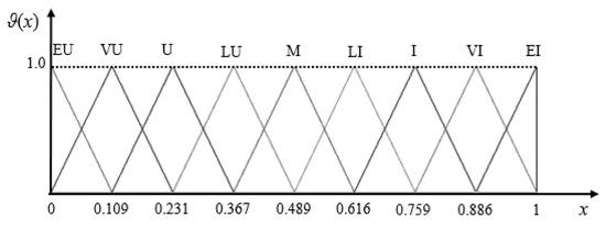
Figure 1. An illustrative example of the TFSs of $\mathrm{t}\mathrm{h}\mathrm{e} F_{L_k}$ (k = 2) structure.

3. A Linguistic Framework for Dynamic MCGDM

3.1. Dynamic MCGDM Problem

In practice, many problems require periodic evaluation over successive time periods. This issue was modeled by Campanella and Ribeiro [32] and was referred to as the dynamic MCGDM problem. In this paper, we propose a framework to address this problem based on the integration and enhancement of the fuzzy weight determination method (FAHP) and the ranking method (FTOPSIS, HA-TOPSIS). The semantics of L-words are represented using a 4-tuple semantic model. The improved methods are referred to as L-FAHP and L-FTOPSIS, respectively.

Assume that at period t, $\mathrm{w}\mathrm{h}\mathrm{e}\mathrm{r}\mathrm{e} t=1,\dots ,T(T\ge 1),$ we have three sets: ${\stackrel{⃛}{A}}^t$ = $\left\{A_1^t,A_2^t,\dots ,A_{m_t}^t\right\}$, ${\stackrel{⃛}{C}}^t$= $\left\{C_1^t,C_2^t,\dots ,C_{n_t}^t\right\}$, and ${\stackrel{⃛}{D}}^t$= $\left\{D_1^t,D_2^t,\dots ,D_{h_t}^t,\right\},$ which represent the sets of alternatives, criteria, and experts. For an expert $D_e^t,$ where e = 1, 2, …, $h_t$ ($h_t$ $\ge 1$), the evaluation of an alternative $A_i^t$, i = 1, 2, …, $m_t$ ($n_t\ge 1$) on an criteria $C_j^t,$ j = 1, 2, …, $n_t$ ($n_{t }\ge 1$) is considered.

At each period t, the $h_t$experts agree on the L-scale $L_k$ (${\stackrel{⃛}{C}}^t$) used to compare the importance levels between pairs of criteria, and they simultaneously agree on the L-scale $L_k$(${\stackrel{⃛}{A}}^t$) used to evaluate the alternatives, according to each criterion. For each expert, $D_e$

(i) Construct the triangular pairwise comparison matrix

$$P_{D_e}^t={(p_{i,j}^e(t))}_{n_t\times n_t}=\left(\begin{array}{cccc}{w}^e(t)& p_{\mathrm{1,2}}^e(t)& \dots & p_{1,n_t}^e(t)\\ & w^e(t)& \dots & p_{2,n_t}^e(t)\\ & & \ddots & ⋮\\ & & & w^e(t)\end{array}\right)$$

(3)

where $p_{i,j}^e(t)\in L_k$(${\stackrel{⃛}{C}}^t$) and $w^e\left(t\right)$is the neutral element of $L_k$ (${\stackrel{⃛}{C}}^t$).

(ii) Construct the alternatives’ rating matrix

$$A_{D_e}^t={\left(a_{i,j}^e(t)\right)}_{m_t\times n_t}=\left(\begin{array}{cccc}{a}_{\mathrm{1,1}}^e(t)& a_{\mathrm{1,2}}^e(t)& \dots & a_{1,n_t}^e(t)\\ a_{\mathrm{2,1}}^e(t)& a_{\mathrm{2,2}}^e(t)& \dots & a_{1,n_t}^e(t)\\ ⋮& ⋮& \ddots & ⋮\\ a_{m_t,1}^e(t)& a_{m_t,2}^e(t)& \dots & a_{m_t,n_t}^e(t)\end{array}\right)$$

(4)

where $a_{i,j}^e(t)$ ∈ $L_k({\stackrel{⃛}{A}}^t$).

From the pairwise comparison matrices and the alternatives’ rating matrices provided by the experts, the ranking of the alternatives is computed. An essential step in this process is the aggregation of L-matrices. To facilitate this aggregation, we introduce an L-aggregation operator, defined on the 4-tuple L-scale.

3.2. Aggregation Operation on 4-Tuple Linguistic Scales

We observe that, over the set of real numbers, for any two real numbers, $a$and $b$, their sum $a+b$ satisfies the following properties:

(i) a + b ≥ a and a + b ≥ b if a, b ≥ 0.

(ii) a + b ≤ a and a + b if a, b ≤ 0.

(iii) a ≤ a + b ≤ b if a ≤ 0 and b ≥ 0 or b ≤ a + b ≤ a if b ≤ 0 and a ≥ 0.

Motivated by this property and the uninorm operation in fuzzy logic, and according to the positive–negative properties of HA, we construct a binary aggregation operator on $L_k$to ensure that the computation results exhibit properties that are analogous to addition over real numbers.

Definition 9. 

Let two L-words $\ddot{x},\ddot{y}\in L_k$be represented by their 4-tuple semantics as $\ddot{x}=\left(x,S_{\left(k\right)}\left(x\right),\vartheta \left(x\right),r_x\right)$and $\ddot{y}=(y,S_{\left(k\right)}(y),\vartheta (y),r_y)$, with $w$being the neutral element of $L_k$. Denote $\ddot{z}=(z,S_{\left(k\right)}(z),\vartheta (z),r_z)$ as the L-word resulting from aggregating $\ddot{x}$ and $\ddot{y}$, denoted by $\ddot{z}=\ddot{x}\oplus \ddot{y}$. The components of $\ddot{z}$are determined as follows:

$$r_z=r_x+{ r}_y=\left\{\begin{array}{c}fm\left(c^{-}\right) \times T({\displaystyle \frac{r_x}{fm(c^{-})}},{\displaystyle \frac{r_y}{fm(c^{-})}}) if x,y < \mathrm{w} \\ fm(c^{-}) + fm(c^{+})\times S({\displaystyle \frac{r_x - fm\left(c^{-}\right)}{fm\left(c^{+}\right)}}, {\displaystyle \frac{r_y - fm(c^{-})}{fm(c^{+})}}) if \mathrm{w}\le x, y \\ {\displaystyle \frac{fm(y)}{fm\left(x\right) + fm(y)}}\times r_{x }+ {\displaystyle \frac{fm(x)}{fm\left(x\right) + fm(y)}}\times r_y if x<\mathrm{w}<y \mathrm{and} x \ne 0, y \ne 1 \end{array}\right.$$

(5)

where T(a, b) = a × b and S(a, b) = a + b − a × b

In Equation (5), the binary operator ⨁ is explicitly defined through three mutually exclusive cases, based on the positions of $x$and $y$relative to the neutral element $\omega$of the L-scale $L_k$. Let $r_x=v\left(x\right)$, $r_y=v\left(y\right)$, and $r_{\omega }=v\left(\omega \right)$denote their respective quantitative semantics. The three cases are described as follows:

Case 1 (both on the negative side of $\omega$): $r_x<r_{\omega }$and $r_y<r_{\omega }$. In this case, the first branch of Equation (5) is applied to compute $r_z$.

Case 2 (both on the non-negative side of $\omega$): $r_x\ge r_{\omega }$and $r_y\ge r_{\omega }$. In this case, the second branch of Equation (5) is applied.

Case 3 (mixed case): Either $r_x<r_{\omega }\le r_y$or $r_y<r_{\omega }\le r_x$. In this case, the third branch of Equation (5) is employed, where $r_z$is computed as a convex combination of $r_x$and $r_y,$weighted according to their fuzziness measures.

Equivalently, by introducing the sign function $\zeta g\eta (\cdot )$, defined on the centered quantitative semantics, $\zeta g\eta \left(x\right)=\zeta g\eta \left(r_x-r_{\omega }\right)\in \left\{-\mathrm{1,0},+1\right\},$we have the following: Case 1 corresponds to $\zeta g\eta \left(x\right)=\zeta g\eta \left(y\right)=-1$; Case 2 corresponds to $\zeta g\eta \left(x\right),\zeta g\eta \left(y\right)\in \{0,+1\}$; and Case 3 includes all remaining combinations, i.e., at least one of $\zeta g\eta \left(x\right), \zeta g\eta \left(y\right)$is $(-1)$ and the other is in $\left\{0,+1\right\}$. Consequently, these three branches of Equation (5) provide a complete and mutually exclusive partitioning of $L_k\times L_k$, ensuring that the operator $\oplus$is well-defined for any pair of L-words.

The component $z$of $\ddot{z }$ is an L-word belonging to $X_{\left(k\right)}$, such that $r_z\in S_{\left(k\right)}\left(z\right)\subseteq L_k$, and $\vartheta \left(z\right)$ represents the quantitative value of the L-word $z$.

Example 2. 

Let us revisit the HA from Example 1. We use Definition 5 to calculate the interval semantics $S_{\left(2\right)}\left(x\right)$for each x ∈ $X$₍₂₎ in the L-scale $L_2$as follows:

$S_{\left(2\right)}$(EU) = [0.1, 0.146), $S_{\left(2\right)}$(VU) = [0.146, 0.256), $S_{\left(2\right)}$(U) = [0.256, 0.366), $S_{\left(2\right)}$(LU) = [0.366, 0.488), $S_{\left(2\right)}$(M) = [0.488, 0.594), $S_{\left(2\right)}$(LI) = [0.594, 0.722), $S_{\left(2\right)}$(I) = [0.722, 0.837), $S_{\left(2\right)}$(VI) = [0.837, 0.952), $S_{\left(2\right)}$(EI) = [0.952, 1].

Applying Definitions 6 to 8, we obtain an L-scale $L_2$ whose semantics are represented by a 4-tuple semantic in Table 1, as follows.

Table 1. L-words and 4-tuple semantic representation of word set X₍₂₎.

L-Words	4-Tuple Sematic
EU	(EU, 0, [0, 0.051), 0)
VU	(VU, 0.109, [0.051, 0.173), 0.109)
U	(U, 0.231, [0.173, 0.295), 0.231)
LU	(LU, 0.367, [0.295, 0.431), 0.367)
M	(M, 0.489, [0.431, 0.549), 0.489)
LI	(LI, 0.616, [0.549, 0.692), 0.616)
I	(I, 0.759, [0.692, 0.819), 0.759)
VI	(VI, 0.886, [0.819, 0.946), 0.886)
EI	(EI, 1, [0.946, 1], 1)

(i) For $\ddot{x}$ = (U, 0.231, [0.173, 0.295), 0.231) and $\ddot{y}$ = (LU, 0.367, [0.295, 0.431), 0.367), we have x, y < w. Therefore, we use the first component formula in Equation (5):

$$\begin{gathered} r_z=fm\left(c^{-}\right)\times T\left({\displaystyle \frac{r_x}{fm\left(c^{-}\right)}},{\displaystyle \frac{r_y}{fm\left(c^{-}\right)}}\right)=0.489\times {\displaystyle \frac{0.231}{0.489}}\times {\displaystyle \frac{0.367}{0.489}}=0.173\in S_{\left(2\right)}\left(U\right) =[0.173, 0.295) \\ \ddot{z}= \ddot{x}\oplus \ddot{y}=(\mathrm{U}, 0.231, [0.173, 0.295), 0.231) \end{gathered}$$

(ii) For $\ddot{x}$ = (I, 0.759, [0.692, 0.819), 0.759) and $\ddot{y}$ = (VI, 0.886, [0.819, 0.946), 0.886), we have x, y > w. Therefore, we use the second component formula in Equation (5).

$$\begin{array}{l}{r}_z=0.489+0.511\times \left[{\displaystyle \frac{0.27}{0.511}}+{\displaystyle \frac{0.397}{0.511}}-{\displaystyle \frac{0.27}{0.511}}\times {\displaystyle \frac{0.397}{0.511}} \right]=0.946 \in S_{\left(2\right)}(EI) = [0.946, 1]\\ \ddot{z}=\ddot{x}\oplus \ddot{y}=(EI, 1, [0.946, 1] 1)\end{array}$$

(iii) For $\ddot{x}$ = (VU, 0.109, [0.051, 0.173), 0.109) and $\ddot{y}$ = (LI, 0.616, [0.549, 0.692), 0.616), we have x < w and y > w. Therefore, we use the third component formula in Equation (5).

$$\begin{gathered} r_z={\displaystyle \frac{fm\left(LI\right)}{fm\left(VU\right)+fm\left(LI\right)}}\times v(VU)+{\displaystyle \frac{fm(VU)}{fm(VU)+fm(LI)}}\times v(LI) \\ {r}_z={\displaystyle \frac{0.270}{0.231+0.270}}\times 0.109+{\displaystyle \frac{0.231}{0.231+0.270}}\times 0.616=0.342 \in S_{\left(2\right)}(LU) = [0.295, 0.431), \\ \ddot{z}=\ddot{x}\oplus \ddot{y}=(LU, 0.367, [0.295, 0.431), 0.342) \end{gathered}$$

Proposition 1. 

For all $\ddot{x}$, $\ddot{y}$ ∈ $L_k$, the aggregation operation ⊕ defined in Definition 6 satisfies the following properties:

(i) It is a closed operation on $L_k$, i.e.,$\ddot{z}$=$\ddot{x}$ ⊕ $\ddot{y}$ ∈$L_k$;

(ii) It satisfies the commutative property, i.e.,$\ddot{x}$ ⊕ $\ddot{y}$=$\ddot{y}$ ⊕ $\ddot{x}$;

(iii) It satisfies the monotonicity property, i.e., if$\ddot{x}$₁ ⪯ $\ddot{x}$₂ then $\ddot{x}$₁ ⊕ $\ddot{y}$ ⪯ $\ddot{x}$₂ ⊕ $\ddot{y}$;

(iv) There exists an identity element, $\ddot{w}$ ∈ $L_k$, such that $\ddot{x}$⊕ $\ddot{w}$ = $\ddot{w}$⊕ $\ddot{x}$ = $\ddot{x}$;

(v) It satisfies the associative property only in the case where all operands lie on the same side of w, i.e., if x, y, z > w or x, y, z < w then ($\ddot{x}$⊕ $\ddot{y}$) ⊕ $\ddot{z}$ = $\ddot{x}$ ⊕  ($\ddot{y}\oplus \ddot{z}$).

Proof. 

According to the definition of HA, we have w = fm($c^{-}$) = θ and fm($c^{-}$) = 1 − θ. Let $r_x=v\left(x\right)$, $r_y=v\left(y\right)$, $r_z=v\left(z\right),$and $r_w=v\left(w\right)$. The HA 4-tuple semantics and the SQM are order-preserving, so it is sufficient to prove the statements for the real-valued aggregation $F\left(r_x,r_y\right)$induced by Equation (5) and then lift the results back to the L-words. We will use these values in the proof below:

(i)

Closure property of the operation

To prove that the operation ⊕ is closed on $L_k$, we only need to show that $r_z$∈ [0, 1], where r_z is calculated according to Equation (5).

Case 1: For x, y < w, the value r_z is computed by using the first formula in Equation (5). The aggregation operator, ⊕, is implemented via an aggregation function, T, on the numerical representatives: $r_z$ = θ × T($r_x$, $r_y$), where T: [0, 1] × [0, 1] ⟶ [0, 1] is a uninorm-type aggregation function. Construction T maps any input pair in ${[0,1]}^2$ to a value in [0, 1]. Therefore, $r_z$ ∈ [0, 1]. This proves that $r_z$ lies in [0, 1].

Case 2: For x, y > w, in which r_z is computed using the second formula in Equation (5). According to Definition 8,

$$r_z=\theta +(1 - 1)S({\displaystyle \frac{r_{x-\theta }}{1-\theta }},{\displaystyle \frac{r_{x-\theta }}{1-\theta }}),$$

where S: [0, 1] × [0, 1] ⟶ [0, 1] is an aggregation operator (uninorm-type), mapping any pair in ${[0,1]}^2$ to a value in [0, 1]. Because θ ≤ $r_z$ ≤ 1, we have 0 < ${\displaystyle \frac{r_{x - \theta } }{1 - \mathsf{\theta }}}$≤ 1. The same holds for ${\displaystyle \frac{r_{y - \theta }}{1 - \mathsf{\theta }}}$. Hence, the two arguments of S lie in [0, 1]. By the codomain of S, S(${\displaystyle \frac{r_{x - \theta }}{1 - \mathsf{\theta }}},{\displaystyle \frac{r_{x - \theta }}{1 - \mathsf{\theta }}})$∈ [0, 1]. Multiply by the nonnegative factor 1 − θ and add θ. Since 0 ≤ 1 − θ ≤ 1 and θ ∈ [0, 1], it follows that 0 ≤ θ + (1 − θ) · 0 ≤ r_z ≤ θ + (1 − θ) · 1 ≤ 1. This proves that $r_z$lies in [0, 1].

Case 3: For x > w > y or x < w < y$,$ in which $r_z$ is computed by using the third formula in Equation (5), we have fm(x) > 0 and fm(y) > 0 => fm(x) + fm(y) > 0.

Let $\alpha ={\displaystyle \frac{fm\left(y\right)}{fm\left(x\right)+fm\left(y\right)}}$, $\beta ={\displaystyle \frac{fm\left(x\right)}{fm\left(x\right)+fm\left(y\right)}}$

So $\alpha + \beta =$ 1. The given formula can be written as $r_z$ = α$r_x$+ β$r_y$, so $r_z$ is a convex combination of $r_x$ and $r_y.$ Because $r_x$, $r_y$∈ [0, 1] and α, β > 0 with α + β = 1, basic properties of convex combinations imply min {$r_x$, $r_y$} ≤ $r_z$ ≤ max {$r_x$, $r_y$}. Since both endpoints lie in [0, 1], it follows that $r_z$ ∈ [0, 1]. Therefore, $r_z$ ∈ [0, 1], as required.

(ii)

Prove the commutative property of the operation

Case 1: $r_x$, $r_y$< θ by definition $r_z$ = T($r_x$, $r_y$). Since T is commutative, T($r_x$, $r_y$) = T($r_y$, $r_x$), hence, $r_x$⊕ $r_y$ = $r_y$⊕ $r_x$, in this case.

Case 2: $r_x$, $r_y$ ≥ θ. Write the normalized arguments u = ${\displaystyle \frac{r_x - \mathsf{\theta }}{1 - \mathsf{\theta }}}$ and v = ${\displaystyle \frac{r_y - \mathsf{\theta }}{1 - \mathsf{\theta }}}$.

Then, $r_z$ = θ + (1 − θ)S(u, v).

Because S is commutative, S(u, v) = S(v, u), so swapping $r_x$ and $r_y$ leaves $r_z$ unchanged. Therefore, the operator is commutative in this case.

Case 3 (mixed): Without loss of generality, assume $r_x$ ≤ θ ≤ $r_y$. The formula gives $r_z = {\displaystyle \frac{fm\left(y\right)}{fm\left(x\right)+ fm\left(\mathrm{y}\right)}}{r}_x + {\displaystyle \frac{fm\left(x\right)}{fm\left(x\right)+ fm\left(\mathrm{y}\right)}}{r}_y$

If we swap x and y, the formula becomes ${r’}_z = {\displaystyle \frac{fm\left(x\right)}{fm\left(x\right) + fm\left(\mathrm{y}\right)}}{r}_y + {\displaystyle \frac{fm\left(y\right)}{fm\left(x\right) + fm\left(\mathrm{y}\right)}}{r}_y$, which is algebraically identical to the previous expression because the denominators are equal and the two words are the same but permuted. Thus, $r_z$ = ${r’}_z;$ therefore, the mixed-case aggregation is commutative.

(iii)

It satisfies the monotonicity property

Equation (5) defines three cases, depending on the positions of $x$and $y$relative to $w$.

Case 1 (both on the negative side of $\mathrm{w}$): When $x,y<w$, the first branch of Equation (5) is used and can be written as

$$r_{x\oplus y}=r_w\hspace{0.17em}T\left({\displaystyle \frac{r_x}{r_w}},{\displaystyle \frac{r_y}{r_w}}\right),$$

where $T\left(a,b\right)=a\cdot b$is the product t-norm. For fixed $y$, the function $r_x\mapsto T\left({\displaystyle \frac{r_x}{r_w}},{\displaystyle \frac{r_y}{r_w}}\right)$is increasing on $\left[0, r_w\right]$; hence, if $r_{x_1}\le r_{x_2}$, then $r_{x_1\oplus y}\le r_{x_2\oplus y}$. The argument is symmetrical in the second argument.

Case 2 (both on the non-negative side of $\mathrm{w}$): When $x,y\ge w$, the second branch of Equation (5) is used. Define the normalized values

$$u_x={\displaystyle \frac{r_x-r_w}{1-r_w}},u_y={\displaystyle \frac{r_y-r_w}{1-r_w}},$$

and

$$r_{x\oplus y}=r_w+(1-r_w)\hspace{0.17em}S(u_x,u_y),$$

where $S\left(a,b\right)=a+b-ab$is the probabilistic sum (a standard t-conorm). The function $S$is increasing in each argument on [0, 1]; therefore, monotonicity holds, as in Case 1.

Case 3 (mixed case): When $x$and $y$lie on different sides of $w$(or one equals $w$), the third branch of Equation (5) is applied and has the following form:

$$r_{x\oplus y}={\displaystyle \frac{fm\left(x\right)\hspace{0.17em}{r}_x+fm\left(y\right)\hspace{0.17em}{r}_y}{fm\left(x\right)+fm\left(y\right)}},$$

where $fm\left(\cdot \right)$denotes the fuzziness measure defined earlier. For fixed $y$, this is a linear (convex) function of $r_x$with a positive coefficient ${\displaystyle \frac{\mathrm{f}\mathrm{m}\left(x\right)}{\mathrm{f}\mathrm{m}\left(x\right)+\mathrm{f}\mathrm{m}\left(y\right)}}$; hence, it is increasing in $r_x$. The argument is symmetrical in $y$.

Combining the three cases and using the order-preserving semantics,$\oplus$is monotone in each argument on $L_k$.

(iv)

An identity element exists: $\ddot{w}$∈ ${\mathrm{L}}_{\mathrm{k}}$

Let $w$be the neutral L-word on $L_k$, with $r_w=v\left(w\right)$and $\mathrm{f}\mathrm{m}\left(w\right)=0$.

If $x\ge w$, then the pair (x, w) is computed according to Case 2. Using $u_w={\displaystyle \frac{r_w-r_w}{1-r_w}}=0$, we obtain

$$r_{x\oplus w}=r_w+(1-r_w)\hspace{0.17em}S\left({\displaystyle \frac{r_x-r_w}{1-r_w}},0\right)=r_w+(1-r_w)\hspace{0.17em}{\displaystyle \frac{r_x-r_w}{1-r_w}}=r_x$$

If $x\le w$, then the pair (x, w) is computed by the mixed case (Case 3). Since $\mathrm{f}\mathrm{m}\left(w\right)=0$, we have

$$r_{x\oplus w}={\displaystyle \frac{\mathrm{f}\mathrm{m}\left(x\right)\hspace{0.17em}{r}_x+\mathrm{f}\mathrm{m}\left(w\right)\hspace{0.17em}{r}_w}{\mathrm{f}\mathrm{m}\left(x\right)+\mathrm{f}\mathrm{m}\left(w\right)}}={\displaystyle \frac{\mathrm{f}\mathrm{m}\left(x\right)\hspace{0.17em}{r}_x}{\mathrm{f}\mathrm{m}\left(x\right)}}=r_x$$

Thus, in all cases, the quantitative semantics of $x\oplus w$equals $r_x$, and by commutativity, we also have $w\oplus x=x$. Therefore, $w$is the identity element of $\oplus$.

(v)

It satisfies the associative property only in the case where all operands lie on the same side of w, i.e., when x, y, z > w or x, y, z < w, then ($\ddot{\mathrm{x}}$ ⊕ $\ddot{\mathrm{y}}$) ⊕ ż = $\ddot{\mathrm{x}}$ ⊕ ($\ddot{\mathrm{y}}$⊕ ż).

We consider the positions of $x,y,z$with respect to the neutral element $w$.

If all three L-words lie on the same side of $w$ (either $x,y,z<w$or $x,y,z\ge w$), then Equation (5) reduces to compositions of the product t-norm, $T$, (for the negative side) or the probabilistic sum, $S,$(for the non-negative side) on the normalized quantitative semantics. Both $T$and $S$ are associative on [0, 1]. Hence, in this situation,

$$r_{(x\oplus y)\oplus z}=r_{x\oplus (y\oplus z)},$$

and, by the order-preserving property of the 4-tuple semantics,

$$\left(x\oplus y)\oplus z=x\oplus (y\oplus z\right).$$

This completes the proof that the aggregation operator $\oplus$ is associative in the case where all operands lie on the same side of w (either $x,y,z<w$or $x,y,z\ge w$).

Note that the aggregation operator $\oplus$ is associative when all operands lie on the same side of the neutral element w: that is, when Equation (5) is evaluated entirely within a single branch. In this case, $\oplus$ reduces to the product t-norm for operands smaller than w and to the probabilistic sum for operands greater than w, both of which are associative. When operands are taken from different sides of w, Equation (5) switches to the mixed branch, and associativity is no longer guaranteed, reflecting the semantic distinction between negative and non-negative linguistic values encoded by the neutral element. Accordingly, to ensure consistent and reproducible aggregation results in the mixed case, operands are arranged in ascending order before applying $\oplus .$ This operational convention preserves determinism without affecting the applicability of the proposed operator in practical aggregation scenarios. □

Definition 10. 

Let n L-words $\ddot{x_j}\in L_k$, j = 1, …, n, be represented by their 4-tuples as $\ddot{x_j}=(x_j,S_{\left(k\right)}(x_j),\vartheta (x_j),r_{x_j})$ and assume that the $\ddot{x_j}$ are arranged in ascending order to the value $x_j$. Denote by $\ddot{z}=(z,S_{\left(k\right)}(z),\vartheta (z),r_z)$ the L-word resulting from aggregating all $\ddot{x_i}$, denoted by $\ddot{z}=\sum _{j=1}^n\ddot{x_j}$. The components of $\ddot{z }$ are determined as follows:

$$\ddot{z}={\sum }_{j=1}^n\ddot{x_j}={\sum }_{j=1}^{n-1}\ddot{x_j}\oplus \ddot{x_n}$$

(6)

For convenience in presenting the algorithm in the following section, we introduce the concept of the empty L-word, denoted by ∅ = {}. We define the aggregation of an L-word from the scale $L_k$ with the empty word, as follows.

Definition 11. 

Let an L-word $\ddot{x}$ ∈${ L}_k$ be represented by its 4-tuple $\ddot{x}=(x,S_{\left(k\right)}(x),\vartheta (x),r_x)$, with w being the neutral element of $L_k$. Let $\ddot{z}=(z,S_{\left(k\right)}(z),\vartheta (z),r_z)$ be the L-word resulting from aggregating $x$with the empty word ∅. Then, $\ddot{z}$ is defined as follows:

$$\ddot{z}=\varnothing \oplus \ddot{x}=\ddot{x}$$

(7)

$$\ddot{z}=\ddot{x} \oplus \varnothing$$

(8)

The components of $\ddot{z}$ are determined as follows:

$$r=v\left(\mathit{w}\right)+\alpha (r_x-v(\mathit{w}\left)\right)$$

(9)

where α∈ [0, 1] is the semantic decay rate (or forgetting rate when applied to dynamic MCGDM) of the aggregation operator when $\ddot{x}$ is combined with ∅. The component z of $\ddot{z}$ is an L-word belonging to $X_{\left(k\right)}$, such that $r_z$ ∈ $S_{\left(k\right)}\left(z\right)$, and v(z) is the quantitative value of the L-word z.

Equation (9) is designed as a simple, semantically transparent model for the temporal decay of an L-word toward the neutral element w when we aggregate it with the empty L-word defined in Definition 11. At the quantitative semantics level, let $r_x=v\left(x\right)$and $r_{\mathit{w}}=v\left(\mathsf{\omega }\right)$. When a historical evaluation is missing at period $t$, we formally denote this absence using the symbol $\mathrm{\varnothing }$ and apply the decay operator

$$r_z=r_w+\lambda \hspace{0.17em}(r_x-r_w),\lambda \in [0, 1],$$

to attenuate the influence of the last available value $r_{x }$towards the neutral element,$r_w$.

It is important to note that $\mathrm{\varnothing }$ is not an actual L-word on the scale $L_k$; it is only a formal symbol indicating the absence of a current evaluation. Therefore, it does not have its own quantitative semantics, and we do not define any value $v\left(\mathrm{\varnothing }\right)$. Instead, the neutral element w provides the unique semantic baseline used in the decay mechanism.

The parameter, $\lambda$, serves as a semantic decay (or forgetting) rate. For $\lambda =1,$there is no decay, and thus, $r_z=r_x$. For $\lambda =0,$the information is fully forgotten, resulting in $r_z=r_w$. For values of $\lambda$ strictly between 0 and 1 ($0<\lambda <1),$the value $r_z$lies strictly between $r_x$and $r_w$, modeling a progressive loss of influence of the historical evaluation. Repeated application of this operator produces an exponential-type attenuation towards $r_w$, a standard and well-understood behavior in dynamic decision models.

3.3. A Novel Linguistic Framework for Dynamic MCGDM

In this paper, we propose an L-framework for addressing the dynamic MCGDM problem, consisting of two main phases: (i) determining the weights of criteria and (ii) ranking the alternatives. In both phases, experts employ 4-tuple semantic L-scales to perform pairwise comparisons of the criteria and evaluate the alternatives. The L-aggregation problem is handled using an L-aggregation operator defined on the 4-tuple semantics L-scale, while fuzzy semantics are employed to compute the criteria weights and determine the ranking of alternatives.

In Phase 1, we introduce the L-FAHP model, developed as an extension of the FAHP method proposed in [21,34], to determine the criteria weights. In Phase 2, we propose the L-FTOPSIS model, extended from the FTOPSIS approach in [47,48], to rank the alternatives. The proposed framework aims to address the dynamic MCGDM problem in a periodic manner, where the evaluation at the current period $t$relies on both the current and historical data from period t − 1.

Notation: $P_{D_e}^t \mathrm{a}\mathrm{n}\mathrm{d} {\tilde{A}}_{D_e}^t$ denote, respectively, the pairwise comparison matrix and the alternatives’ rating matrix in the L-scale provided by the $e^{th}$expert (e = 1, 2, …, $h_t).$ AP^t, ${A\tilde{A}}^t$ denote the aggregated pairwise comparison matrix and the aggregated alternatives’ rating matrix from all $h_t$experts. $\overline{{AP}^t}$ and $\overline{{A\tilde{A}}^t}$ denote the aggregated pairwise comparison matrix and aggregated evaluation matrix combined with historical data (from period t − 1); $F\overline{{AP}^t} \mathrm{a}\mathrm{n}\mathrm{d} F\overline{{A\tilde{A}}^t}$ denote the aggregated pairwise comparison matrix and the aggregated alternatives’ rating matrix after integration with historical data, whose values are expressed as fuzzy set semantics of the L-words. Figure 2 below provides an overview of the steps in the L-framework for the dynamic MCGDM problem.

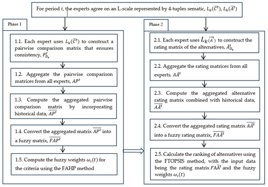
Figure 2. The linguistic framework for dynamic MCGDM.

In the following section, the detailed steps for each phase are presented. Note that the aggregation operator used in this framework is the aggregation operator for L-words represented by 4-tuples, as defined by Equations (5)–(9).

• Phase 1. Determining criterion weights in dynamic MCGDM

Step 1.1. Each expert $e^{th}$uses the L-words x ∈ $X_k$ from the L-scale $L_k$(${\stackrel{⃛}{C}}^t$) (defined in Example 2) to construct the pairwise comparison matrix of the criteria, $P_{D_e}^t$, structured as shown in Equation (3). The consistency of the matrix $P_{D_e}^t$ is then verified by transforming the L-matrix $P_{D_e}^t$ into a fuzzy matrix ${FP}_{D_e}^t$ through mapping each element $p_{i,j}^t$(t) of $P_{D_e}^t$to its corresponding element in ${FP}_{D_e}^t$, using the mapping fz($p_{i,j}^t$(t)). The consistency of the fuzzy matrix ${FP}_{D_e}^t$is subsequently checked, and if it does not satisfy the consistency condition, $P_{D_e}^t$ is adjusted iteratively until the condition is met.

The consistency of each pairwise comparison matrix is assessed by calculating its consistency ratio (CR), as defined in Equation (10):

$${CR}^t= {\displaystyle \frac{{CI}^t}{RI}}$$

(10)

where Kien et al. [31] introduced the formula in which CI is the consistency index, as defined in Equation (11).

$${CI}^t={\displaystyle \frac{{\lambda }_{max}^t-\left(n_t-\left(1-w^t\right)\right)}{\left(n_t-\left(1-w^t\right)\right) }}$$

(11)

Here ${\lambda }_{max}^t is$the maximum eigenvalue, $n^t$ is the number of criteria, and $w^t$ represents the semantic quantification of the neutral element w at period t in the HA. The RI values are provided in Table 2.

Table 2. Random index values (RI).

n	1	2	3	4	5	6	7	8	9	10	11	12	13	14	15
RI	0.00	0.00	0.58	0.90	1.12	1.24	1.32	1.41	1.45	1.49	1.51	1.54	1.56	1.57	1.59

When the CR of the $e^{th}$ pairwise comparison matrix is computed to be greater than or equal to 0.10 (CR $\ge 0.10)$, it indicates inconsistency in the experts’ judgments. In such cases, the $e^{th}$ expert is required to reassess and revise the matrix until the recalculated CR reaches an acceptable level, specifically below 0.10 (CR < 0.10)).

Step 1.2. Aggregate the pairwise comparison matrices from all experts, ${AP}^{\mathit{t}}$

$${AP}^t={({\tilde{p}}_{i,j}(t))}_{n_t\times n_t}$$

(12)

Each element of the matrix ${AP}^t$is determined as follows.

$${\tilde{p}}_{i,j}(t)=p_{i,j}^1(t)\oplus p_{i,j}^2(t)\oplus \dots \oplus p_{i,j}^{h_t}(t)\hspace{1em}\hspace{1em}(i, j=1,\dots ,n_t)$$

(13)

Step 1.3. Compute the aggregated pairwise comparison matrix by incorporating historical data, $\overline{{AP}^t}$, for t > 1.

The notation ${\stackrel{⃛}{C}}_u^t$ represents the set of attributes from periods $t-1$and $t$: that is, ${\stackrel{⃛}{C}}_u^t$ = ${\stackrel{⃛}{C}}^{t-1}$∪ ${\stackrel{⃛}{C}}^t$ $\mathrm{a}\mathrm{n}\mathrm{d} n_t^u$denotes the cardinality of the set. Equation (14) is used to determine the elements on the aggregated pairwise comparison matrix, incorporating historical data.

$${\tilde{p}\ast }_{i,j}\left(t\right)=\left\{\begin{array}{c}\varnothing \oplus {\tilde{p}}_{i,j}\left(t\right) \mathrm{if} C_i^{t-1}\notin {\stackrel{⃛}{C}}^{t-1 }\mathrm{and} C_i^t\in {\stackrel{⃛}{C}}^t, \\ {\tilde{p}}_{i,j}\left(t-1\right)\oplus {\tilde{p}}_{i,j}\left(t\right) \mathrm{if} C_i^{t-1}, C_i^t\in {\stackrel{⃛}{C}}^{t-1}\cap {\stackrel{⃛}{C}}^t, \\ {\tilde{p}}_{i,j}\left(t-1\right)\oplus \varnothing C_i^{t-1}\in {\stackrel{⃛}{C}}^{t-1} \mathrm{and} C_i^{t-1}\notin {\stackrel{⃛}{C}}^t\end{array}\right. i, j=1, \dots , n_t^u$$

(14)

Step 1.4. Construct a triangular fuzzy semantic comparison matrix of L-words

Definition 8 is applied to transform the elements of the fuzzy matrix $\overline{{AP}^t}$ into the fuzzy matrix $\overline{F{AP}^t}$, as illustrated in Equation (15) below:

$$\overline{F{AP}^t} = {({\widetilde{fp}\ast }_{i,j}\left(t\right) )}_{n_t\times n_t}=\left(\begin{array}{cccc}fz({\tilde{p}\ast }_{\mathrm{1,1}}\left(t\right))& fz({\tilde{p}\ast }_{\mathrm{1,2}}\left(t\right))& \dots & fz({\tilde{p}\ast }_{1{,n}_t}\left(t\right))\\ fz({\tilde{p}\ast }_{\mathrm{2,1}}\left(t\right))& fz({\tilde{p}\ast }_{\mathrm{2,2}}\left(t\right))& \dots & fz({\tilde{p}\ast }_{2{,n}_t}\left(t\right))\\ ⋮& ⋮& \ddots & ⋮\\ fz({\tilde{p}\ast }_{n_t,1}\left(t\right))& fz({\tilde{p}\ast }_{n_t,2}\left(t\right))& \dots & fz({\tilde{p}\ast }_{n_t{,n}_t}\left(t\right))\end{array}\right)$$

(15)

where $fz({\tilde{p}\ast }_{i,j}\left(t\right))={(l}_{i,j}(t), m_{i,j}(t),u_{i,j}(t)), fz\left({\widetilde{p^{-1}}\ast }_{i,j}\left(t\right)\right)= \left({{\displaystyle \frac{1}{u}}}_{i,j\left(t\right)}, {{\displaystyle \frac{1}{m}}}_{i,j\left(t\right)},{{\displaystyle \frac{1}{l}}}_{i,j\left(t\right)}\right),$ $for i, j=1, \dots , n_t and i\ne j,$fz is the mapping of the TFS of an L-word, as seen in Figure 1.

To prevent zero denominators when computing inverse values in the pairwise comparison matrix, the obtained values are rescaled from the range [0, 1] to the interval [0.1, 1]. Table 3 presents the TFSs of L-words used to compare the relative importance of two criteria.

Table 3. TFSs of L-words for comparing the importance of two criteria.

Order	L-Words	TFSs of L-Words Based on HA	Reciprocal TFSs of L-Words Based on HA
1	EU	(0.1, 0.1, 0.198)	(1/0.198, 1/0.1, 1/0.1)
2	VU	(0.1, 0.198, 0.308)	(1/0.308, 1/0.198, 1/0.1)
3	U	(0.198, 0.308, 0.430)	(1/0.430, 1/0.308, 1/0.198)
4	LU	(0.308, 0.430, 0.540)	(1/0.540, 1/0.430, 1/0.308)
5	M	(0.430, 0.540, 0.654)	(1/0.654, 1/0.540, 1/0.430)
6	LI	(0.540, 0.654, 0.783)	(1/0.783, 1/0.654, 1/0.540)
7	I	(0.654, 0.783, 0.897)	(1/0.897, 1/0.783, 1/0.654)
8	VI	(0.783, 0.897, 1)	(1, 1/0.897, 1/0.783)
9	EI	(0.897, 1, 1)	(1, 1, 1/0.897)

Step 1.5. The fuzzy weights and the normalized weights of each criterion are obtained using Buckley’s geometric mean approach [34].

First, the geometric mean of the fuzzy pairwise comparison values for criterion i with respect to all other criteria is calculated, as expressed in Equation (16):

$$\overline{R{AP}_i^t} = {\left( \prod _{j=1}^{n_t}{\widetilde{fp}\ast }_{i,j}\left(t\right)\right)}^{1/n_t}, i=1, 2, \dots , n_t$$

(16)

Subsequently, the fuzzy weight of the $i^{th}$criterion, expressed as a triangular fuzzy number, is derived according to Equation (17).

$${\omega }_i\left(t\right)=\overline{R{AP}_{i }^t}\left(t\right)\otimes {\left(\overline{R{AP}_1^t}\left(t\right)\oplus \overline{R{AP}_2^t}\left(t\right) \oplus \dots \oplus \overline{R{AP}_n^t}\left(t\right)\right)}^{-1}=\left(l{\omega }_i\left(t\right), {m\omega }_i\left(t\right), {u\omega }_i\left(t\right) \right)$$

(17)

Defuzzification is performed using the center of area (COA) method, through which the representative crisp value $M_i\left(t\right)$ of each fuzzy weight ${\omega }_i\left(t\right)$is obtained, as specified in Equation (18).

$${\mathrm{M}}_{\mathrm{i}}\left(\mathrm{t}\right)={\displaystyle \frac{l{\omega }_i\left(t\right)+{m\omega }_i\left(t\right)+{u\omega }_i\left(t\right)}{3}},{\mathrm{w}\mathrm{h}\mathrm{e}\mathrm{r}\mathrm{e} \mathrm{M}}_{\mathrm{i}}\left(\mathrm{t}\right) \mathrm{i}\mathrm{s} \mathrm{a} \mathrm{n}\mathrm{o}\mathrm{n}\mathrm{f}\mathrm{u}\mathrm{z}\mathrm{z}\mathrm{y} \mathrm{n}\mathrm{u}\mathrm{m}\mathrm{b}\mathrm{e}\mathrm{r}.$$

(18)

The weights of the criteria and sub-criteria, ${\mathrm{M}}_{\mathrm{i}}\left(\mathrm{t}\right),$ are then obtained by normalizing these crisp values.

• Phase 2. Ranking of the alternatives

The ranking of alternatives is determined by using the Fuzzy TOPSIS method, with the input data being the rating matrix $\overline{{F\mathrm{A}\tilde{\mathrm{A}}}^t}$and the fuzzy weights ${\omega }_i\left(t\right).$

Step 2.1. Each expert uses the L-words x ∈ $X_k$, obtained from the L-scale ${\mathrm{L}}_{\mathrm{k}}({\stackrel{⃛}{A}}^t$) (defined in Table 4), to construct the rating matrix of the alternatives, ${\tilde{A}}_{D_e}^t$, structured as in Equation (4).

Table 4. The 4-tuple L-scales for rating alternatives.

Order	L-Words	4-Tuple Semantic	TFSs of L-Words Based on HA
1	Extremely Low (EL)	(EL, 0.1, [0.1, 0.219), 0.1)	(0.1, 0.1, 0.336)
2	Low (L)	(L, 0.336, [0.219, 0.450), 0.336)	(0.1, 0.336, 0.566)
3	Medium (M)	(M, 0.566, [0.450, 0.675), 0.566)	(0.336, 0.566, 0.781)
4	High (H)	(H, 0.781, [0.675, 0.889), 0.781)	(0.566, 0.781, 1)
5	Extremely High (EH)	(EH, 1, [0.889, 1], 1)	(0.781, 1.000, 1)

Step 2.2. Aggregate the rating matrices from all experts, ${A\tilde{A}}^t$

$${A\tilde{A}}^t={\left({\tilde{a}}_{i,j}\right(t\left)\right)}_{m_t\times n_t}$$

(19)

Each element of the matrix ${A\tilde{A}}^t$ is determined as follows.

$${\tilde{a}}_{i,j}\left(t\right)=a_{i,j}^1\left(t\right)\oplus a_{i,j}^2\left(t\right)\oplus \dots \oplus a_{i,j}^{h_t}\left(t\right); (i=1,\dots , m_t, j=1,\dots ,n_t)$$

(20)

Step 2.3. Compute the aggregated alternative rating matrix combined with historical data, $\overline{{A\tilde{A}}^t}$, for t > 1

The notation ${\stackrel{⃛}{A}}_u^t$ represents the set of attributes from periods $t-1,$ and $t$, that is, ${\stackrel{⃛}{A}}_u^t$ = ${\stackrel{⃛}{A}}^{t-1}$∪ ${\stackrel{⃛}{A}}^t$, $\mathrm{a}\mathrm{n}\mathrm{d} m_t^u$ denotes the cardinality of the set. Equation (21) is used to determine the elements of the aggregated rating matrix that incorporates historical data:

$${\tilde{a}\ast }_{i,j}\left(t\right)=\left\{\begin{array}{c}\varnothing \oplus {\tilde{a}}_{i,j}\left(t\right) {\displaystyle \genfrac{}{}{0pt}{}{{if [A}_i\in {\stackrel{⃛}{A}}^t\backslash {\stackrel{⃛}{A}}^{t-1} \mathrm{and}{ C}_j\in {\stackrel{⃛}{C}}^t\backslash C^{t-1}] or [A_i\in {\stackrel{⃛}{A}}^{t-1}\backslash {\stackrel{⃛}{A}}^t \mathrm{and}{ C}_j \in {\stackrel{⃛}{ C}}^t\backslash C^{t-1}]}{or [A_i\in {\stackrel{⃛}{A}}^{t-1}\backslash {\stackrel{⃛}{A}}^t \mathrm{and} C_j\in {\stackrel{⃛}{C}}^t\backslash C^{t-1}]}}\\ {\tilde{a}}_{i,j}\left(t-1\right)\oplus {\tilde{a}}_{i,j}\left(t\right) if{A}_i\in {\stackrel{⃛}{A}}^t\cap {\stackrel{⃛}{A}}^{t-1} \mathrm{and} C_j\in {\stackrel{⃛}{C}}^t\cap C^{t-1} \\ {\tilde{a}}_{i,j}\left(t-1\right)\oplus \varnothing if{A}_i\in {\stackrel{⃛}{A}}^{t-1}\backslash {\stackrel{⃛}{A}}^t \mathrm{and} C_j\in {\stackrel{⃛}{C}}^{t-1}\backslash C^t \end{array}\right.$$

(21)

Step 2.4. Convert the aggregated rating matrix ${A\tilde{A}}^t$ into a fuzzy rating matrix, ${F\mathrm{A}\tilde{\mathrm{A}}}^t$.

Use Equation (22), the elements of the fuzzy matrix $\overline{{F\mathrm{A}\tilde{\mathrm{A}}}^t}$are computed as follows:

$${\widetilde{fa}\ast }_{i,j}\left(t\right) = fz\left({\tilde{a}\ast }_{i,j}\left(t\right)\right),i=1,\dots , m_t^u,j = 1, \dots , n_t^u$$

(22)

where fz is the mapping of the triangular fuzzy semantics of an L-word, as defined in Definition 8.

Step 2.5. The weighted normalized decision matrix is calculated using Equation (23), below:

$$T_i^t= {\displaystyle \frac{1}{n}}\sum _{j= 1}^{n_t^u}{\omega }_i\left(t\right) {\widetilde{fa}\ast }_{i,j}\left(t\right), i = 1, \dots , m_t^u, j = 1, \dots , n_t^u$$

(23)

Step 2.6. The distances of the alternatives from the positive ideal solution (PIS, ${\mathcal{B}}^{+})$and the negative ideal solution (NIS, ${\mathcal{B}}^{-})$at period t are determined using Equations (24) and (25):

$$T_i^{+t}= \sqrt{{(T_i^t-{\mathcal{B}}^{+})}^2 }, i = 1, \dots , m_t^u,$$

(24)

$$T_i^{-t}=\sqrt{{(T_i^t-{\mathcal{B}}^{-})}^2 }, j=1, \dots , n_t^u$$

(25)

where ${\mathcal{B}}^{+}=\left(1, 1, 1\right), {\mathcal{B}}^{-}= \left(0, 0, 0\right), i = 1, \dots , m_t^u$ and $T_i^{+t}$ and $T_i^{-t}$ represent the distances from the positive and negative ideal solutions of each alternative, respectively.

Step 2.7. Calculation of the closeness coefficients and ranking of alternatives.

The closeness coefficient at period t is computed using Equation (26). The alternatives are then ranked according to their T$C_i^{+t}$ values, where a larger T$C_i^{+t}$ indicates a better-performing alternative:

$$\mathrm{T}{C}_i^{+t}= {\displaystyle \frac{T_i^{-t}}{T_i^{+t} + T_i^{-t}}}$$

(26)

4. Application of the Proposed Framework to Evaluate the Digital Transformation Levels of Enterprise

In this section, an application for evaluating the digital transformation levels of small- and medium-sized enterprises (SMEs) in the retail sector in Vietnam is presented to demonstrate the effectiveness of the proposed method.

To assess the digital transformation levels of retail enterprises, previous studies have identified a comprehensive set of critical criteria across four major dimensions. In terms of technology and digital capabilities, enterprises need to emphasize their ability to integrate and implement digital platforms such as e-commerce, Big Data, IoT, and blockchain [49], as well as their capacity to deploy artificial intelligence (AI), cloud computing, and data-driven decision-making using large-scale analytics [44]. Within the strategy and organization dimension, the establishment of a clear digital transformation strategy with explicit objectives and KPIs, accompanied by strong leadership commitment, organizational adaptability, and appropriate resource allocation, are key factors determining the success of digital transformation initiatives [44,45,49]. Regarding customer experience, retail enterprises must strengthen their omnichannel capabilities [45], personalize customer interactions through technology adoption [44], and enhance convenience and transaction speed in digital services to meet increasingly demanding customer expectations [44]. Finally, in terms of human resources and culture, investing in digital skill development and training, fostering an innovation-driven culture, encouraging risk-taking, and adjusting organizational structures to support digital transformation are essential prerequisites for ensuring the sustainability and effectiveness of this process [50].

Overall, this set of criteria not only reflects the current status and capabilities of digital transformation within retail enterprises but also serves as a vital foundation for developing appropriate strategies to optimize operations and enhance competitiveness in today’s digitized business environment.

The input data for the proposed approach were collected through semi-structured interviews with top managers and department heads of the selected enterprises. Following a preliminary screening process, ten enterprises (denoted as DN1 to DN10) were chosen for analysis. According to the L-scales ${\mathrm{L}}_{\mathrm{k}}({\stackrel{⃛}{A}}^t$) and ${\mathrm{L}}_{\mathrm{k}}({\stackrel{⃛}{C}}^t$), shown in Table 1 and Table 4, respectively, experts provided ratings for the ten enterprises and determined the criteria weights using four criteria and fourteen sub-criteria to assess the digital transformation levels of SMEs in Vietnam’s retail sector. The definitions of these criteria and sub-criteria are provided in Table 5.

Table 5. Criteria for evaluating the digital transformation level of retail SMEs in Vietnam.

Criteria	Sub-Criteria
Strategy and Organization (S_O)	(S_O1) Clear digital transformation strategy with specific objectives and measurable key performance indicators (KPIs).
	(S_O2) Organizational flexibility and adaptability to technological change.
	(S_O3) Appropriate allocation of resources for digital initiatives (investment in technology, human resources, and employee training).
Technology and Digital Capabilities (T_D)	(T_D1) Integration and utilization of digital platforms (e-commerce, big data, IoT, blockchain, etc.).
	(T_D2) Artificial intelligence capabilities (machine learning, recommender systems, customer analytics).
	(T_D3) Use of cloud computing for data and software services.
	(T_D4) Data-driven decision-making, using big data and predictive analytics.
Customer Experience (C)	(C1) Omnichannel capability integrating online and offline interactions.
	(C2) Personalization and targeted digital marketing (customized products and personalized customer experiences).
	(C3) Enhanced customer interactions using augmented reality, virtual reality, and AI-driven personalization.
	(C4) Convenient and fast digital transactions (fast delivery, click and collect, mobile payments).
Human Resources and Culture (H_C)	(H_C1) Training and development of employees’ digital skills and continuous learning.
	(H_C2) Organizational culture that supports innovation, risk taking, and digital transformation.
	(H_C3) Impact of digital transformation on employment structure (more skilled workers and digitally aligned structures).

Suppose that Province A in Vietnam intends to rank the digital transformation performance of SMEs over different periods. The alternatives and evaluation criteria are allowed to vary in response to changes in the external environment. A committee of three experts (denoted as D₁, D₂, and D₃), each with extensive knowledge and experience in developing and evaluating digital transformation initiatives for SMEs in Vietnam, is responsible for determining the relative importance of the criteria and rating the alternatives. The evaluation process involved three rounds of questionnaires administered to the experts at three distinct time periods (t₁, t₂, t₃). In addition, the retention policy preserves all alternatives from A_t to H_t and carries all elements of the matrix $P_{D_e}^t \mathrm{a}\mathrm{n}\mathrm{d}$ ${\tilde{A}}^t$ forward to the next period; however, only the alternatives available in each specific period are considered for ranking at the end of that period.

For simplicity, our proposed DGMCDM framework is illustrated by using three time periods (t₁, t₂, t₃).

(1) 

Period t₁:

The experts evaluated five enterprises (a₁, a₂, a₃, a₄, a₅). Based on an analysis of the current context, eleven sub-criteria grouped under three main criteria, namely strategy and organization, technology and digital capabilities, and customer experience, were identified for assessment. Table A1, Table A2, Table A3, Table A4, Table A5 and Table A6 in Appendix A present the fuzzy comparison matrix for the criteria and sub-criteria, as well as the aggregated evaluations of the enterprises and the importance weights of the criteria at period t₁. Table 6 and Table 7 illustrate the computational steps of the decision-making model at time t₁, including the calculation of the weighted average assessments of the enterprises, their distances to the PIS and NIS, and the closeness coefficients of the enterprises. Table 8 reports the resulting ranking of the enterprises, in which enterprise DN2 emerges as the best alternative.

Table 6. Weighted average rating of enterprises in period t₁.

Enterprises	Weighted Average Ratings
DN1	(0.047, 0.111, 0.177)
DN2	(0.061, 0.133, 0.185)
DN3	(0.029, 0.080, 0.149)
DN4	(0.025, 0.072, 0.135)
DN5	(0.028, 0.076, 0.141)

Table 7. Distances of enterprises from $B^{+}$ and B⁻ in period t₁.

Enterprises	${\mathit{d}}^{+}$	${\mathit{d}}^{-}$
DN1	0.890	0.124
DN2	0.875	0.136
DN3	0.915	0.099
DN4	0.924	0.090
DN5	0.919	0.094

Table 8. Closeness coefficients and ranking of enterprises in period t₁.

Enterprises	Closeness Coefficients	Ranking
DN1	0.122	2
DN2	0.135	1
DN3	0.098	3
DN4	0.088	5
DN5	0.093	4

(2) 

Period ${\mathit{t}}_2$:

At this stage, three new enterprises (DN6, DN7, DN8) were added, and three sub-criteria under the main criterion human resources and culture were incorporated into the survey. The computational procedures for aggregating the enterprise assessments and combining the importance weights of the fourteen criteria are presented in Table A7 and Table A8 in the Appendix A. Table 9 and Table 10 report the results of the computation, including the weighted average evaluations of the enterprises, their distances from the PIS and the NIS, the closeness coefficients, and the resulting rankings. The final ranking of the enterprises is given in Table 11, in which DN6 is identified as the best alternative.

Table 9. Weighted average rating of enterprises in period $t_2$.

Enterprises	Weighted Average Ratings
DN1	(0.023, 0.054, 0.111)
DN2	(0.025, 0.058, 0.114)
DN3	(0.019, 0.047, 0.103)
DN4	(0.014, 0.037, 0.090)
DN5	(0.015, 0.040, 0.092)
DN6	(0.030, 0.066, 0.112)
DN7	(0.022, 0.052, 0.112)
DN8	(0.016, 0.043, 0.095)

Table 10. Distances of the enterprises from $B^{+}$ and B⁻ in period t₂.

Enterprises	${\mathit{d}}^{+}$	${\mathit{d}}^{-}$
DN1	0.938	0.072
DN2	0.935	0.075
DN3	0.944	0.067
DN4	0.954	0.057
DN5	0.952	0.058
DN6	0.931	0.077
DN7	0.939	0.072
DN8	0.949	0.061

Table 11. Closeness coefficients and ranking of enterprises in period $t_2$.

Enterprises	Closeness Coefficients	Ranking
DN1	0.072	3
DN2	0.075	2
DN3	0.066	5
DN4	0.056	8
DN5	0.058	7
DN6	0.077	1
DN7	0.072	4
DN8	0.060	6

(3) 

Period ${\mathit{t}}_3$:

At the beginning of this period, enterprises DN1 and DN2 were removed from the set of alternatives for practical reasons, and two new enterprises, DN9 and DN10, were introduced into the model. The criteria set remained the same as in the second period, consisting of 14 sub-criteria grouped into four main criteria. Table A9 and Table A10 in Appendix A present, respectively, the aggregated evaluation ratings of the enterprises and the importance weights of the 14 sub-criteria. Table 12 and Table 13 then describe the computational procedure, including the weighted average ratings, the distances from each enterprise to the PIS and NIS, the resulting closeness coefficients, and the final ranking of the enterprises. Finally, Table 14 reports the consolidated ranking of the 10 enterprises, in which DN2 is identified as the optimal alternative.

Table 12. Weighted average rating of enterprises in period $t_3$.

Enterprises	Weighted Average Ratings
DN1	(0.018, 0.046, 0.094)
DN2	(0.034, 0.070, 0.115)
DN3	(0.011, 0.032, 0.075)
DN4	(0.015, 0.038, 0.086)
DN5	(0.020, 0.046, 0.095)
DN6	(0.030, 0.062, 0.105)
DN7	(0.029, 0.060, 0.105)
DN8	(0.020, 0.046, 0.095)
DN9	(0.031, 0.063, 0.105)
DN10	(0.028, 0.059, 0.103)

Table 13. Distances of the enterprises from $B^{+}$and B⁻ in period t₃.

Enterprises	${\mathit{d}}^{+}$	${\mathit{d}}^{-}$
DN1	0.948	0.061
DN2	0.928	0.080
DN3	0.961	0.047
DN4	0.954	0.055
DN5	0.947	0.062
DN6	0.935	0.073
DN7	0.936	0.072
DN8	0.947	0.062
DN9	0.934	0.073
DN10	0.937	0.071

Table 14. Closeness coefficients and ranking of enterprises in period $t_3$.

Enterprises	Closeness Coefficients	Ranking
DN1	0.061	8
DN2	0.079	1
DN3	0.047	10
DN4	0.054	9
DN5	0.061	7
DN6	0.072	3
DN7	0.071	4
DN8	0.062	6
DN9	0.073	2
DN10	0.070	5

5. A Comparative Analysis

This subsection provides a comparative analysis to assess the proposed methodology’s effectiveness and robustness. Table 15, Table 16 and Table 17 present the digital transformation rankings of enterprises in periods t₁, t_1-2, and t_1-3, using the integrated dynamic fuzzy AHP-TOPSIS approach proposed by Quynh [51]. The results show that in period t₁, enterprises DN2 and DN1 are ranked first and second, respectively, which aligns with the outcomes derived from the proposed approach. In period t_1-2, the rankings for enterprises DN2, DN4, DN6, and DN7 are also consistent with those from the proposed approach. Similarly, in period t_1-3, the rankings from both methods match for enterprises DN6, DN3, and DN4.

Table 15. Enterprise rankings in period t₁, using the approach presented in [51].

Enterprises	Weighted Average Ratings	${\mathit{d}}^{+}$	${\mathit{d}}^{-}$	Closeness Coefficients	Ranking
DN1	(0.139, 0.202, 0.264, 0.298; 0.600)	0.932	0.281	0.231	2
DN2	(0.186, 0.258, 0.330, 0.365; 0.600)	0.862	0.351	0.290	1
DN3	(0.107, 0.167, 0.228, 0.265; 0.600)	0.972	0.241	0.199	5
DN4	(0.113, 0.176, 0.240, 0.277; 0.600)	0.961	0.253	0.209	4
DN5	(0.109, 0.176, 0.244, 0.281; 0.600)	0.960	0.256	0.210	3

Table 16. Enterprise rankings in period $t_{1-2}$ (average of t₁ and t₂), using the approach presented in [51].

Enterprises	Weighted Average Ratings	${\mathit{d}}^{+}$	${\mathit{d}}^{-}$	Closeness Coefficients	Ranking
DN1	(0.129, 0.196, 0.263, 0.300; 0.600)	0.937	0.278	0.229	5
DN2	(0.156, 0.229, 0.301, 0.339; 0.600)	0.896	0.319	0.262	2
DN3	(0.114, 0.178, 0.243, 0.282; 0.600)	0.958	0.257	0.2114	7
DN4	(0.112, 0.177, 0.243, 0.282; 0.600)	0.959	0.256	0.211	8
DN5	(0.114, 0.185, 0.255, 0.294; 0.600)	0.949	0.268	0.220	6
DN6	(0.182, 0.264, 0.345, 0.386; 0.600)	0.852	0.366	0.300	1
DN7	(0.137, 0.205, 0.273, 0.314; 0.600)	0.925	0.290	0.239	4
DN8	(0.128, 0.210, 0.292, 0.333; 0.600)	0.916	0.304	0.249	3

Table 17. Enterprise rankings in period $t_{1-3}$ (average of t₁, t₂ and t₃), using the approach presented in [51].

Enterprises	Weighted Average Ratings	${\mathit{d}}^{+}$	${\mathit{d}}^{-}$	Closeness Coefficients	Ranking
DN1	(0.129, 0.196, 0.263, 0.300; 0.600)	0.9369	0.2777	0.2286	7
DN2	(0.169, 0.246, 0.323, 0.363; 0.600)	0.8748	0.3417	0.2809	4
DN3	(0.114, 0.178, 0.243, 0.282; 0.600)	0.9580	0.2569	0.2115	10
DN4	(0.120, 0.190, 0.259, 0.299; 0.600)	0.9431	0.2730	0.2245	9
DN5	(0.120, 0.192, 0.264, 0.305; 0.600)	0.9395	0.2776	0.2281	8
DN6	(0.161, 0.244, 0.327, 0.369; 0.600)	0.8752	0.3437	0.2820	3
DN7	(0.133, 0.204, 0.275, 0.318; 0.600)	0.9247	0.2916	0.2398	6
DN8	(0.137, 0.218, 0.298, 0.341; 0.600)	0.9067	0.3125	0.2563	5
DN9	(0.209, 0.288, 0.366, 0.402; 0.600)	0.8252	0.3899	0.3209	1
DN10	(0.165, 0.251, 0.338, 0.382; 0.600)	0.8649	0.3553	0.2912	2

However, ranking discrepancies between the two approaches are observed in other cases. The application of HA and varied semantic representations of linguistic assessments enhances semantic interpretability and robustness, complementing rather than duplicating traditional fuzzy logic methods.

6. Sensitivity Analysis and Discussion

In this study, a two-scenario sensitivity analysis was conducted to rigorously assess the robustness of the model with respect to both linguistic input perturbations and variations in the HA parameters. The results indicate that the dynamic L-FAHP and L-FTOPSIS framework based on HA maintains a high level of robustness, exhibiting minimal deviation in the final rankings despite the global perturbations applied to the input data. This demonstrates the model’s strong capability in mitigating the semantic uncertainty that is inherent in expert-based linguistic assessments. Overall, these findings substantiate the reliability, stability, and methodological soundness of the proposed approach, confirming its practical suitability for evaluating the digital transformation maturity of retail enterprises in Vietnam. A comprehensive summary of the sensitivity analysis is provided in Table 18 and Figure 3 and Figure 4, below.

Table 18. Comparative ranking results for periods $t_1$, t₂, and t₃.

Period	Original	Ranking After Sensitivity Analysis
		Upward Shift in L-Words by One Level on the L-Scale	HA Fuzziness Adjustment with a One-Level Upward L-Shift
${\mathrm{t}}_1$	DN2 $\succ$ DN1 $\succ$ DN3 $\succ$ DN5 $\succ$ DN4	DN2 $\succ$ DN1 $\succ$ DN3 $\succ$ DN5 $\succ$ DN4	DN2 $\succ$ DN1 $\succ$ DN3 $\succ$ DN5 $\succ$ DN4
${\mathrm{t}}_2$	DN6 $\succ$ DN2 $\succ$ DN1 $\succ$ DN7 $\succ$ DN3 $\succ$ DN8 $\succ$ DN5 $\succ$DN4	DN6 ≻ DN2 ≻ DN7 ≻ DN1 ≻ DN3 ≻ DN8 ≻ DN5 ≻ DN4	DN6 $\succ$ DN2 $\succ$ DN7 $\succ$ DN1 $\succ$ DN3 $\succ$ DN8 $\succ$ DN5 $\succ$DN4
${\mathrm{t}}_3$	DN2 $\succ$ DN9 $\succ$ DN6 $\succ$ DN7 $\succ$ DN10 $\succ$ DN8 $\succ$ DN5 $\succ$ DN1 $\succ$ DN4 $\succ$ DN3	DN2 ≻ DN9 ≻ DN6 ≻ DN7 ≻ DN10 ≻ DN8 ≻ DN5 ≻ DN1 ≻ DN4 ≻ DN3	DN2 $\succ$ DN9 $\succ$ DN6 $\succ$ DN7 $\succ$ DN10 $\succ$ DN1 $\succ$ DN8 $\succ$ DN5 $\succ$ DN4 $\succ$ DN3

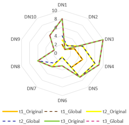
Figure 3. Sensitivity analysis global perturbation scenario.

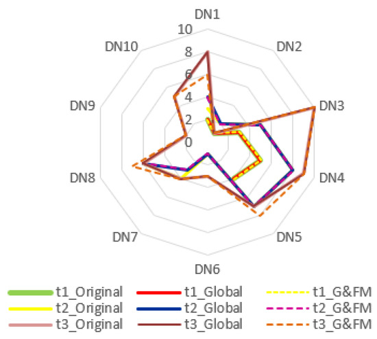
Figure 4. Semantic sensitivity of the HA-based MCGDM to global perturbations and fuzziness parameter changes.

In Scenario 1, all pairwise comparison judgments for the 14 sub-criteria under the four main criteria were systematically perturbed by shifting each linguistic term upward by one level on the L-scale in Table 1. The comparative ranking results for periods $t_1,t_2,$and $t_3$are reported in Table 18, with the corresponding radar plots shown in Figure 3, below.

Despite structural changes in the decision space across periods, ranging from eleven criteria and five SMEs in$\mathrm{p}\mathrm{e}\mathrm{r}\mathrm{i}\mathrm{o}\mathrm{d} t_1$ to fourteen criteria and eight SMEs in period $t_2$, and subsequently, ten SMEs in period $t_3,$ the ranking outcomes under both the original and the globally perturbed scenarios remain largely consistent. In period $t_1$, all SMEs retain their ranking positions after perturbation, confirming that the HA-based L-scaling and weighting mechanism yields stable priority vectors, even under systematic scale distortions. In period $t_2,$ although the decision space expands, only minor shifts are observed (for example, DN1 and DN3 shifting by one position). This indicates moderate yet controlled sensitivity without significantly affecting the global ranking structure. By period $t_3$, where only a subset of alternatives (DN1 and DN3) retains historical traces and new SMEs enter the system, the rankings again exhibit a high correspondence between the perturbed and unperturbed scenarios. The closeness coefficient profiles shown in Figure 3 for the original and global (perturbed) cases nearly coincide with all three periods. These findings indicate that the dynamic model based on HA demonstrates only a weak sensitivity to systematic distortions in expert linguistic assessments, thereby producing highly stable group rankings.

In Scenario 2, a more demanding perturbation was considered. The fuzziness parameter values of HA (such as $fm\left(c^{-}\right)=0.5 \mathrm{a}\mathrm{n}\mathrm{d} \mu \left(h^{-}\right)=0.5$) were modified, and simultaneously, all pairwise comparison judgments were shifted upward by one level on the L-scale in Table 1. The radar plots in Figure 4 illustrate three curves for each period: original, global, and global and FM.

Even under this combined perturbation of both the L-data and the underlying HA semantics, the shapes of the curves remain very similar and the leading enterprises retain their positions across periods $t_1,t_2$, and $t_3$. Deviations occur only among certain mid- and low-ranked alternatives (e.g., slight changes in the positions of DN1, DN3, and DN8 at $t_3$), and even these differences are small in magnitude. This confirms that the model is robust not only to changes in expert judgments but also to reasonable variations in the HA quantification parameters.

A prominent strength of the HA-based dynamic MCGDM framework is its ability to explicitly represent the temporal evolution of L-semantics, a capability not inherently supported by conventional fuzzy or neutrosophic approaches. In traditional fuzzy and neutrosophic models, L-information is encoded through externally defined membership or rating functions, which do not capture the generative semantic relationships among L-words and lack formal operators to manage their temporal transformations. In contrast, HA provides an intrinsic semantic structure that enables L-meanings to intensify, weaken, or progressively degrade in response to temporal changes or contextual dynamics. This property is particularly important in digital transformation assessment, where enterprise performance evolves continuously under technological, regulatory, and organizational shifts.

The advantage of HA becomes particularly evident in scenarios where an alternative is removed at period t − 1 but must still be included in the final ranking at period t. Through the HA L-fusion operator ${\tilde{a}}_{i,j}\left(t-1\right)\oplus {\tilde{a}}_{i,j}\left(t\right),$historical assessments are retained rather than discarded. They undergo semantic attenuation governed by the algebraic rule outlined in Definition 8, which ensures that missing or outdated evaluations are transformed into a semantically consistent L-value. This mechanism serves as a formal model of controlled semantic fading, allowing the system to maintain historical information with appropriately reduced influence. Consequently, an alternative excluded in period t − 1 can reappear in the final ranking, with its historical semantic contribution moderated accordingly. This ensures a complete and temporally coherent evaluation process.

Such behavior is difficult to replicate in fuzzy or neutrosophic systems, which lack operators that are capable of modeling data absence, semantic degradation, or generative evolution of L-words across periods. The ability of the HA framework to store, inherit, and transform L-information, even for alternatives that are temporarily absent from the decision space, represents a substantial methodological advantage in dynamic MCGDM contexts. It preserves the semantic trajectory of each alternative and supports a more comprehensive, historically grounded decision-making process.

Overall, the two scenarios collectively demonstrate that the proposed dynamic L-FAHP and L-FTOPSIS framework, based on HA, exhibits a high level of robustness concerning (i) systematic changes in expert linguistic assessments and (ii) reasonable variations in the HA fuzziness parameters. The temporal attenuation of historical information in periods $t_2$and $t_3$ effectively controls the propagation of perturbations over time, ensuring that the model yields stable and interpretable rankings while still accurately capturing the evolving nature of digital transformation maturity among the retail enterprises under study.

7. Conclusions

This study proposed a novel linguistic framework for a dynamic MCGDM grounded in the algebraic semantics of HA. By integrating the HA 4-tuple semantic model with L-FAHP and L-FTOPSIS, a unified and semantically interpretable approach was developed for dynamic decision environments characterized by time-varying information. The main theoretical contributions of the proposed framework can be summarized as follows. First, a two-phase dynamic architecture was introduced to support both time-dependent weight determination and the temporal evaluation of alternatives. Second, HA-based semantic quantification was employed to preserve the inherent ordering and meaning of linguistic terms throughout the computational process, thereby improving semantic consistency and interpretability. Third, a formally defined semantic degradation mechanism was incorporated to manage historical information in dynamic decision-making contexts. Together, these contributions establish a coherent semantic foundation for the considered class of dynamic MCGDM problems.

The applicability of the proposed framework was illustrated through a case study evaluating the digital transformation levels of enterprises across multiple time periods. The results demonstrate that the model is capable of handling changes in criteria, alternatives, and group judgments over time within this application context. A comparative analysis with a representative baseline method indicates that the proposed approach offers improved semantic interpretability and greater flexibility in accommodating temporal dynamics. Furthermore, the sensitivity analysis suggests that the model exhibits stable behavior with respect to variations in key parameters under the examined conditions. These findings indicate that the HA-based dynamic L-FAHP and L-FTOPSIS framework constitutes a viable tool for dynamic decision-making problems involving linguistic information.

Despite these contributions, several limitations should be acknowledged. The effectiveness of the framework depends on the quality and appropriateness of the expert-defined linguistic domains, and the adopted monotonic semantic degradation assumption may not adequately reflect situations in which historical information regains importance. In addition, computational demands may increase in large-scale or high-frequency dynamic settings. Addressing these limitations provides directions for future research. In particular, further work will explore the use of the ComHA fuzziness measure μ(h) to design alternative aggregation operators and investigate convergence properties in long-term dynamic evaluations. Such extensions are expected to further strengthen the theoretical basis of HA-based dynamic MCGDM within the scope of the proposed framework.

References

- Alkan, N.; Kahraman, C. CODAS Extension Using Novel Decomposed Pythagorean, Fuzzy Sets: Strategy Selection for IOT Based Sustainable Supply Chain System. Expert Syst. Appl. 2023, 237, 121534. [Google Scholar] [CrossRef]
- Wang, C.N.; Nguyen, H.P.; Huang, C.C.; Wang, Y.H. Evaluating Interventions in Response to COVID-19 Outbreak by Multiple-Criteria Decision-Making Models. Systems 2022, 10, 68. [Google Scholar] [CrossRef]
- Lazarashouri, H.; Najafi, S.E. Enhancing emergency department efficiency through simulation and fuzzy multi-criteria decision-making integration. J. Oper. Strateg. Anal. 2024, 2, 56–71. [Google Scholar] [CrossRef]
- Sarsangi, V.; Karimi, A.; Hadavandi, E.; Hokmabadi, R. Prioritizing risk factors of hazardous material road transportation accidents using the fuzzy AHP method. Work 2023, 75, 275–286. [Google Scholar] [CrossRef]
- Thong, N.T.; Smarandache, F.; Hoa, N.D.; Son, L.H.; Lan, L.T.H.; Cu, N.G. A Novel Dynamic Multi-Criteria Decision Making, Method Based on Generalized Dynamic Interval-Valued Neutrosophic. Symetry 2020, 12, 618. [Google Scholar] [CrossRef]
- Carrasco, R.A.; Villar, P.; Hornos, M.J.; Herrera-Viedma, E. A Linguistic Multi-Criteria Decision-Making Model Applied to the Integration of Education Questionnaires. Int. J. Comput. Intell. Syst. 2011, 4, 946–959. [Google Scholar]
- Kurniawati, E.; Kohar, U.H.A.; Pirzada, K. Change or destroy: The digital transformation of indonesian MSMEs to achieve sustainable economy. Pol. J. Manag. Stud. 2022, 26, 248–264. [Google Scholar] [CrossRef]
- Li, Z.; Zhang, X.; Tao, Z.; Wang, B. Enterprise digital transformation and supply chain management. Financ. Res. Lett. 2024, 60, 104883. [Google Scholar] [CrossRef]
- Luo, Y.; Cui, H.; Zhong, H.; Wei, C. Business environment and enterprise digital transformation. Financ. Res. Lett. 2023, 57, 104250. [Google Scholar] [CrossRef]
- Zhang, T.; Shi, Z.Z.; Shi, Y.R.; Chen, N.J. Enterprise digital transformation and production efficiency: Mechanism analysis and empirical research. Econ. Res. Ekon. Istraživanja 2021, 35, 2781–2792. [Google Scholar] [CrossRef]
- Su, Y.; Wu, J. Digital transformation and enterprise sustainable development. Financ. Res. Lett. 2024, 60, 104902. [Google Scholar] [CrossRef]
- Li, T.; Wen, J.; Zeng, D.; Liu, K. Has enterprise digital transformation improved the efficiency of enterprise technological innovation? A case study on Chinese listed companies. Math. Biosci. Eng. 2022, 19, 12632–12654. [Google Scholar] [CrossRef] [PubMed]
- Cai, C.; Tu, Y.; Li, Z. Enterprise digital transformation and ESG performance. Financ. Res. Lett. 2023, 589, 104692. [Google Scholar] [CrossRef]
- Brodny, J.; Tutak, M. Assessing the level of digital maturity of enterprises in the Central and Eastern European countries using the MCDM and Shannon’s entropy methods. PLoS ONE 2021, 16, e0253965. [Google Scholar] [CrossRef]
- Huang, Q.; Tang, Y. Enterprise Digital Transformation Strategy: The Impact of Digital Platforms. Entropy 2025, 27, 295. [Google Scholar] [CrossRef] [PubMed]
- Marín Díaz, G. A Fuzzy-XAI Framework for Customer Segmentation and Risk Detection: Integrating RFM, 2-Tuple Modeling, and Strategic Scoring. Mathematics 2025, 113, 2141. [Google Scholar] [CrossRef]
- Herrera, F.; Martínez, L. A 2-tuple fuzzy linguistic representation model for computing with words. IEEE Trans. Fuzzy Syst. 2002, 8, 746–752. [Google Scholar] [CrossRef]
- Jiang, Y. A general type-2 fuzzy model for computing with words. Int. J. Intell. Syst. 2018, 33, 713–758. [Google Scholar] [CrossRef]
- Díaz, G.M.; Salvador, J.L.G. Group Decision-Making Model Based on 2-Tuple Fuzzy Linguistic Model and AHP Applied to Measuring Digital Maturity Level of Organizations. Systems 2023, 11, 341. [Google Scholar] [CrossRef]
- Akram, M.; Noreen, U.; Deveci, M. Enhanced ELECTRE II method with 2-tuple linguistic m-polar fuzzy sets for multi-criteria group decision making. Expert Syst. Appl. 2023, 213, 119237. [Google Scholar] [CrossRef]
- Chang, D.Y. Applications of the extent analysis method on fuzzy AHP. Eur. J. Oper. Res. 1996, 95, 649–655. [Google Scholar] [CrossRef]
- Wang, Y.M.; Luo, Y.; Hua, Z.S. On the extent analysis method for fuzzy AHP and its applications. Eur. J. Oper. Res. 2008, 186, 735–747. [Google Scholar] [CrossRef]
- Büyüközkan, G.; Güleryüz, S. Multi criteria group decision making approach for smart phone selection using intuitionistic fuzzy TOPSIS. Int. J. Comput. Intell. Syst. 2016, 9, 709–725. [Google Scholar] [CrossRef]
- Wang, Y.; Ma, X.; Qin, H.; Sun, H.; Wei, W. Hesitant Fermatean fuzzy Bonferroni mean operators for multi-attribute decision-making. Complex Intell. Syst. 2024, 10, 1425–1457. [Google Scholar] [CrossRef]
- Yang, G.; Ren, M.; Hao, X. Multi-criteria decision-making problem based on the novel probabilistic hesitant fuzzy entropy and TODIM method. Alex. Eng. J. 2023, 68, 437–451. [Google Scholar] [CrossRef]
- Akram, M.; Ramzan, N.; Deveci, M. Linguistic Pythagorean fuzzy CRITIC-EDAS method for multiple-attribute group decision analysis. Eng. Appl. Artif. Intell. 2023, 119, 105777. [Google Scholar] [CrossRef]
- Erdebilli, B.; Yilmaz, I.; Aksoy, T.; Hacioglu, U.; Yüksel, S.; Dinçer, H. An interval-valued Pythagorean fuzzy AHP and COPRAS hybrid methods for the supplier selection problem. Int. J. Comput. Intell. Syst. 2023, 16, 124. [Google Scholar] [CrossRef]
- Chen, T.Y. A point operator-driven approach to decision-analytic modeling for multiple criteria evaluation problems involving uncertain information based on T-spherical fuzzy sets. Expert Syst. Appl. 2022, 203, 117559. [Google Scholar] [CrossRef]
- Long, V.N.; Thong, V.H. Information aggregation problem of 4 tuple linguistic based on hedge algebra. J. Comput. Sci. Cybern. 2012, 27, 241–252. [Google Scholar] [CrossRef]
- Ho, C.N.; Huynh, V.N.; Pedrycz, W. A construction of sound semantic linguistic scales using 4-tuple representation of term semantics. Int. J. Approx. Reason. 2014, 55, 763–786. [Google Scholar] [CrossRef]
- Kien, N.V.; Thong, H.V.; Ho, N.C.; Dat, L.Q. A Novel Integrated Fuzzy Analytic Hierarchy Process with a 4-Tuple Hedge Algebra Semantics for Assessing the Level of Digital Transformation of Enterprises. Mathematics 2025, 13, 3539. [Google Scholar] [CrossRef]
- Li, G.; Kou, G.; Peng, Y. Dynamic fuzzy multiple criteria decision making for performance evaluation. Technol. Econ. Dev. Econ. 2015, 21, 705–719. [Google Scholar] [CrossRef]
- Buckley, J.J. Fuzzy hierarchical analysis. Fuzzy Sets Syst. 1985, 17, 233–247. [Google Scholar] [CrossRef]
- Campanella, G.; Ribeiro, R.A. A framework for dynamic multiple-criteria decision making. Decis. Support Syst. 2011, 52, 52–60. [Google Scholar] [CrossRef]
- Yang, Y.; Jie, M.Q.; Chen, Z.S. Dynamic three-way multi-criteria decision making with basic uncertain linguistic information: A case study in product ranking. Appl. Soft Comput. 2024, 152, 111228. [Google Scholar] [CrossRef]
- Bastanifar, I.; Khan, K.H.; Azmi, S.N.; Opera, E. Applying dynamic TOPSIS: A multi-criteria decision-making approach to economic corridors under uncertainty-the case of IMEEC. Cogent Econ. Financ. 2025, 13, 2558028. [Google Scholar] [CrossRef]
- Zhao, S.; Liu, J.; Kadziński, M.; Liao, X.; Wang, Y. A Probabilistic preference learning approach for multiple criteria ranking in dynamic decision context. Eur. J. Oper. Res. 2025; in press. [Google Scholar] [CrossRef]
- Yang, S.; Liao, H.; Wu, X. Prescriptive analytics for dynamic multi-criterion decision making considering learned knowledge of alternatives. Expert Syst. Appl. 2025, 268, 126350. [Google Scholar] [CrossRef]
- Ho, C.N.; Wechler, W. Hedge algebras: An algebraic approach to structures of sets of linguistic domains of linguistic truth variables. Fuzzy Sets Syst. 1990, 35, 281–293. [Google Scholar] [CrossRef]
- Ho, C.N.; Long, V.N. Fuzziness measure on complete hedges algebras and quantifying semantics of terms in linear hedge algebras. Fuzzy Sets Syst. 2007, 158, 452–471. [Google Scholar] [CrossRef]
- Nguyen, T.D.; Bui, H.L. General optimization procedure of the hedge-algebras controller for controlling dynamic systems. Artif. Intell. Rev. 2023, 56, 2749–2784. [Google Scholar] [CrossRef]
- Ho, C.N.; Thong, H.V.; Long, V.N. A discussion on interpretability of linguistic rule base systems and its application to solve regression problems. Knowl. Based Syst. 2015, 88, 107–133. [Google Scholar] [CrossRef]
- Hieu, D.N.; Phong, D.P. A Novel High-order Linguistic Time Series Forecasting Model with the Growth of Declared Word-set. Int. J. Adv. Comput. Sci. Appl. 2021, 12, 6371. [Google Scholar] [CrossRef]
- Gouveia, F.D.; Mamede, H.S. Digital Transformation for SMEs in the Retail Industry. Procedia Comput. Sci. 2022, 204, 671–681. [Google Scholar] [CrossRef]
- Wadud, I.; Liang, Y.D.; Polkinghorne, M. Digital Transformation in the UK Retail Sector. Encyclopedia 2025, 5, 142. [Google Scholar] [CrossRef]
- Kao, L.J.; Chiu, C.C.; Lin, H.T.; Hung, Y.W.; Lu, C.C. Evaluating the Digital Transformation Performance of Retail by the DEA Approach. Axioms 2022, 11, 284. [Google Scholar] [CrossRef]
- Chen, T.C. Extensions of the TOPSIS for group decision-making under fuzzy environment. Fuzzy Sets Syst. 2000, 114, 1–9. [Google Scholar] [CrossRef]
- Shih, H.S.; Shyur, H.J.; Lee, E.S. An extension of TOPSIS for group decision making. Math. Comput. Model. 2007, 45, 801–813. [Google Scholar] [CrossRef]
- Sobczak, E. Digital Transformation of Enterprises and Employment in Technologically Advanced and Knowledge-Intensive Sectors in the European Union Countries. Sustainability 2025, 17, 5868. [Google Scholar] [CrossRef]
- Liu, T.; Leng, J.; Zhu, S.; Fu, R. Digital Transformation and Enterprise Innovation Capability: From the Perspectives of Enterprise Cooperative Culture and Innovative Culture. J. Theor. Appl. Electron. Commer. Res. 2025, 20, 136. [Google Scholar] [CrossRef]
- Quynh, V.T.N. An integrated dynamic generalized trapezoidal fuzzy AHP-TOPSIS approach for evaluating sustainable performance of bank. Adv. Decis. Sci. 2023, 27, 68–86. [Google Scholar] [CrossRef]
Disclaimer/Publisher’s Note: The statements, opinions and data contained in all publications are solely those of the individual author(s) and contributor(s) and not of MDPI and/or the editor(s). MDPI and/or the editor(s) disclaim responsibility for any injury to people or property resulting from any ideas, methods, instructions or products referred to in the content. |
© 2025 by the authors. Licensee MDPI, Basel, Switzerland. This article is an open access article distributed under the terms and conditions of the Creative Commons Attribution (CC BY) license.