Abstract
This study investigates the horizontal positioning accuracy of a low-cost, multi-frequency GNSS receiver operating in static mode using a newly released PPP-RTK correction service delivering localized corrections. To the authors’ knowledge, this represents one of the first performance evaluations of this service, which optimizes correction data based on the approximate receiver location. The results are compared against those from the previous version of the service, which provided non-localized corrections. Analyses were conducted in both the time and frequency domains, employing robust statistical tools to characterize error behavior. The localized service achieved a mean horizontal error of approximately 0.020 m and a 95% Circular Error Probable (CEP95) of 0.046 m, in line with its declared performance. By contrast, the earlier non-localized service yielded a mean horizontal error of approximately 0.074 m and a CEP95 of 0.124 m under comparable static conditions, confirming the significant improvement achieved by localized corrections. Spectral and wavelet analyses revealed a dominant 33 mHz harmonic in the positioning error, corresponding to the 30 s update period of atmospheric corrections, indicating a periodic influence arising from the correction stream. Continuous wavelet analysis further identified intervals in which this harmonic was absent, during which positioning accuracy improved markedly (CEP95 reduced to 0.019 m). To properly address the non-Gaussian nature of the error distribution, bias-corrected and accelerated (BCa) bootstrap methods were applied to estimate confidence intervals. Overall, the results demonstrate the benefits of localized corrections, while emphasizing the importance of accounting for the temporal structure of correction data in PPP-RTK performance assessments. Future developments will focus on kinematic scenarios and adaptive filtering strategies to mitigate periodic errors induced by correction updates.
1. Overview of PPP-RTK Correction Services
Today, everyday users can benefit from signals transmitted by all four Global Navigation Satellite Systems (GNSSs) [1], which operate across multiple frequency bands. The widespread availability of commercially accessible, low-cost, multi-frequency, multi-constellation GNSS receivers has democratized access to high-precision positioning. Under open-sky conditions, more than 20 satellites are generally visible at any moment, enabling real-time positioning accuracy down to the centimeter level even with low-cost devices [2]. Previously, such accuracy required the use of Real-Time Kinematic (RTK) and Network RTK (NRTK) methods in conjunction with expensive, high-grade receivers. Nowadays, centimeter-level accuracy is achievable with affordable hardware, thanks to the emergence of low-cost RTK-enabled receivers. In addition, commercial correction services are continuously expanding their coverage and improving their performance, further boosting the positioning capabilities of these low-cost solutions. To ensure interoperability across different GNSS receivers and enable real-time corrections, standardized formats and real-time protocols, such as RTCM SSR, have been developed. These standards facilitate consistent data exchange and processing across GNSS devices, supporting communication through satellites, wireless links, and the Internet [3]. RTCM SC-104 introduced RTCM SSR as an industry-standard format to enhance GNSS data interoperability and accuracy. While RTCM version 2 had limitations, RTCM version 3.0 improved message encoding and flexibility. RTCM SSR extends this protocol, providing precise corrections for satellite orbits, clocks, and biases, which helps improve accuracy and reduce convergence times for real-time positioning [4,5]. Similarly, the International GNSS Service (IGS) developed IGS SSR, a format that supports real-time PPP applications and is compatible with RTCM SSR [5,6]. Recent innovations include the Compact State Space Representation (CSSR) and the Secure Position Augmentation for Real-Time Navigation (SPARTN) formats. CSSR, originally designed for QZSS, offers a 70% improvement in bandwidth efficiency over RTCM SSR, making it highly effective for global PPP applications. The development of open standards like SPARTN reflects the growing demand for higher accuracy, reduced latency, and greater interoperability in global positioning systems. These advancements create new opportunities for precise and reliable GNSS applications across diverse industries. The first operational satellite-based PPP-RTK augmentation system was implemented by Japan through the Centimeter-Level Augmentation Service (CLAS), delivered via the Quasi-Zenith Satellite System (QZSS) since November 2018 [7]. Following this pioneering deployment, several countries—including South Korea, Australia, Germany, and Denmark—began exploring and deploying their own PPP-RTK services [8]. At the international level, the European GNSS Galileo has introduced the High-Accuracy Service (HAS), which provides free correction data via the E6-B signal and through terrestrial means such as the Internet. Based on the principles of precise point positioning, Galileo HAS enables sub-meter positioning. As demonstrated by Naciri et al. [9], combined Galileo and GPS solutions achieved horizontal and vertical accuracies below 0.20 m and 0.40 m, respectively, with convergence times of less than 6 min in static mode and 7.5 min in kinematic mode at the 95th percentile. Beginning in the mid-2020s, several private companies entered the market with commercial SSR-based correction services built on PPP-RTK technology. Trimble Inc. deployed the CenterPoint RTX service [10], NovAtel introduced TerraStar-X [11], and u-blox launched PointPerfect [12], targeting applications in automotive, robotics, and industrial IoT. In France, the company Teria developed TeriaSat, a PPP-RTK service that currently offers complete national coverage with L-band geostationary satellite correction delivery [13]. More recently, Swift Navigation introduced Skylark, a state-of-the-art wide-area correction service designed to meet the stringent requirements of automotive applications. Skylark delivers sub-decimeter positioning accuracy with rapid convergence, achieving performance in a matter of seconds across the contiguous United States and Europe [14]. In parallel, public-sector efforts have also advanced. Australia and New Zealand are jointly developing SouthPAN (Southern Positioning Augmentation Network), planning to provide regional PPP-RTK capability [15]. Among the various PPP-RTK services currently available, this study evaluates the latest PPP-RTK correction service developed by u-blox, PointPerfect Flex. We specifically evaluate the localized correction mode of PointPerfect Flex, carrying out a comparison with the previous service. A key advancement of this new release is that the correction data are spatially filtered and optimized on the server side, based on the approximate position of the receiver. The server uses this positional information to deliver a set of corrections that are region specific, targeting only those satellite visibility conditions and error models relevant to the user’s local environment, resulting in increased accuracy. It incorporates enhanced ionospheric modeling, allowing for a more accurate representation of ionospheric delays at the local scale. These improvements contribute to increased positioning accuracy and faster convergence times. The structure of the paper is as follows: the present section provides an overview of the relevant literature on PPP-RTK, focusing on the evolution of SSR commercial services. Section 2 presents the experimental setup, detailing the hardware, software, and positioning techniques employed. Section 3 focuses on data analysis, with a particular emphasis on time series, frequency, and position domains analysis. Section 4 provides a comparison with the previous correction service discussing the results, whereas, finally, Section 5 concludes the paper and outlines directions for future work.
2. Materials and Methods
The hardware used in this study is the u-blox ZED-F9P, a cost-effective, multi-band GNSS receiver with 184 tracking channels. It supports multiple constellations and signal types, including GPS signals on L1 C/A and L2C, GLONASS L1OF and L2OF, Galileo E1B/E1C and E5b, BeiDou B1I and B2I, QZSS L1 C/A, L1S and L2C, as well as SBAS L1 C/A signals. The receiver was connected via an SMA cable to a u-blox ANN-MB active GNSS antenna [16]. Data were collected during a static survey at a known reference point located in Naples, Italy, which provides a quasi-open-sky environment with limited multipath. The measurement session lasted one hour on 6 June 2025, immediately following the release of the updated PointPerfect correction service. To enable a comparative analysis, a second dataset was also considered. It was acquired at the same location using the same hardware setup and antenna and with an earlier version of the PointPerfect service, which did not yet implement localized corrections. This reference dataset, collected on 2 January 2023, proved instrumental for evaluating the impact of the service update as discussed in detail in the comparative analysis section of this paper.
This research continues the work presented in [17,18,19], focusing on real-time high-accuracy positioning using the u-blox PointPerfect Flex correction service.
PointPerfect Flex is the latest version of u-blox’s SSR-based PPP-RTK augmentation service. Unlike previous versions, it can deliver tailored atmospheric corrections based on the rover position. When used in localized mode, the correction server spatially filters the corrections based on the user’s approximate positions included in the NMEA GGA messages sent by the rover every 10 s. The service provides corrections via both IP and L-band channels; this study employs the IP stream. The correction messages include satellite clock corrections every five seconds and satellite orbit, code, and phase biases, and atmospheric corrections every thirty seconds, following the SPARTN 2.0 specification [20]. It also supports third-party GNSS receivers through standardized delivery protocols such as SPARTN 2.0 over MQTT, increasing interoperability beyond proprietary hardware. The solution are calculated in real-time with u-blox U-Center software version 24.01 (August 2022) that receives and applies PointPerfect Flex included in two types of SPARTN messages: Orbit, Clock, Bias (OCB), localized High-Precision Atmosphere Correction (HPAC). The software logs a .ubx file where, among several messages, the HPPOSLLH, containing the high-precision positions, are parsed with a custom MATLAB R2025-b® parser developed to extract such information. Moreover, given that the PointPerfect Flex data correction service delivers the corrections in ITRF2020 (current epoch), a transformation was performed to align the reference frames, e.g., the ETRS89 with the International Terrestrial Reference System (ITRS), to allow accurate comparison between the ground truth and the PPP-RTK solutions. The ground truth coordinates of the reference station were determined in the ETRF2000 reference frame at epoch 2008.0, consistent with the available initial coordinates. Since the results of the PPP-RTK processing via the PointPerfect service are expressed in the ITRF2020 reference frame at the current epoch, an accurate transformation between the two reference frames, including epoch variation, was necessary. To perform this transformation, the ETRF/ITRF Coordinate Transformation Tool (ECTT), available on the EUREF (EUREF Permanent GNSS Network) portal [21], was used. This tool enables the conversion of coordinates and velocities between different realizations of ETRFxx and ITRFyy, accounting for tectonic drift using the official station velocities. In the absence of specific velocity values for the Naples station, the values available for the MATE00ITA (Matera) station, located approximately 198 km from Naples, shown in Table 1, were used. Although this choice may introduce a residual systematic bias due to geodynamic differences between the two locations, it was necessary in the absence of local velocity data. Despite being an approximation, this approach allowed for the update of the “true” position coordinates from ETRF2000 at epoch 2008.0 to ITRF2020 at the current epoch, ensuring compatibility with the PPP-RTK results and enabling a consistent evaluation of positioning errors.

Table 1.
Velocity of the Matera station (MATE00ITA), from the EPN database.
3. Data Analysis
This section presents a comprehensive analysis of the positioning errors obtained from the static PPP-RTK test using PointPerfect Flex corrections. Both statistical and graphical tools are employed to investigate the temporal behavior and distributional properties of the East and North error components. Particular attention is given to assessing the presence of systematic biases, evaluating distribution normality, and quantifying uncertainty through robust non-parametric methods. The bootstrap approach, specifically the bias-corrected and accelerated (BCa) method, is introduced to construct reliable confidence intervals, motivated by the non-Gaussian nature of the residuals.
Figure 1 shows the temporal evolution of the error for the East coordinate (top panel) and the North one (bottom panel). Once ambiguity resolution was achieved, it remained fixed throughout the experiment, indicating that all solutions in Figure 1 were fixed-ambiguity. The yellow horizontal line represents the mean error, providing a visual reference for assessing both the dispersion of the measurements with respect to the mean value and the presence of a bias. The error analysis revealed the presence of systematic bias, indicated by a sample mean—albeit small—different from zero. For the East error, we found a mean value of 0.0112 m with a standard deviation of 0.0176 m, while for the North one a mean of −0.004 m with a standard deviation of 0.011 m. Since these estimates are derived from a finite sample and are thus subject to variability, we employed a methodology to provide a reliable measure of their precision; therefore, a confidence interval-based approach was adopted.
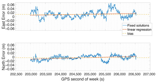
Figure 1.
Temporal evolution of the error on the East coordinate for all fixed-type solutions (top panel), shown in blue. The yellow horizontal line represents the mean error, while the red one represents linear regression trend. The bottom panel shows the corresponding error evolution for the North coordinate, with the same color conventions.
In addition to the mean and standard deviation, the analysis also includes the median and median absolute deviation (MAD). Indeed, the median is particularly useful when dealing with asymmetric distributions or datasets with outliers. Being less sensitive to outliers than the standard deviation, the MAD provides a more reliable estimate of variability in contexts involving non-Gaussian or contaminated data. The joint use of the median and MAD thus allows for a more robust and comprehensive description of the analyzed data distribution.
In particular, to select the most appropriate procedure for calculating the confidence intervals, a preliminary analysis was conducted to assess the plausibility of the normality assumption in the error distribution. This analysis was initially performed using exploratory graphical tools, such as the histogram overlaid with the theoretical normal curve (with mean and variance matching the sample values) and the quantile–quantile plot (QQ-plot).
Figure 2 (left panel) displays the histogram of the East component error, revealing a moderately asymmetric empirical distribution characterized by a pronounced central peak and an extended right tail. The overlaid theoretical normal distribution (red curve), estimated using the sample mean and standard deviation, provides a reasonable fit in the central region but fails to capture the behavior in the tails. In particular, the right tail exhibits a higher frequency of extreme values than predicted under the normality assumption. The QQ-plot in Figure 3 (right panel) clearly highlights how the data diverges from the expected distribution. The central quantiles mostly follow the reference line, but both the lower and upper ends veer away noticeably, creating an “S”-shaped curve. This pattern points to a distribution that is more peaked than a normal one (leptokurtic) and skewed to the right. These characteristics align well with the clustering of errors around 0.012 m and the presence of some large positive outliers observed in the data. In comparison, the North component error (Figure 3, left panel) exhibits a more symmetric distribution, centered around a sample mean of approximately –0.004 m. The histogram shows a slight skewness toward negative values and a flatter shape than the normal distribution. The corresponding QQ-plot (Figure 3, right panel) supports these observations, with the quantiles more closely following the reference line across the distribution but still showing slight deviations at the extremes. In both cases, the tails show clear deviations from normality that, although significant, are relatively modest, indicating that the error distributions are only slightly asymmetric and do not display pronounced heavy tails. To quantitatively support the visual analyses, the Lilliefors test was employed—an extension of the Kolmogorov–Smirnov test particularly suitable for moderately sized samples with unknown parameters [22]. A significance level of = 0.05 was adopted that is a standard value in statistical literature [23]. The null hypothesis of normality was rejected with high significance (p = 0.001) for both the East and North components, confirming that both error distributions significantly deviate from a normal distribution. Given the notable departure of residual error distributions from Gaussianity, the non-parametric bias corrected and accelerated bootstrap method (BCa) was employed [24,25], allowing robust inference even in the presence of distributions influenced by non-Gaussianity, asymmetry, or outliers. A resampling procedure with replacement was implemented using 10,000 replicates, consistent with the literature recommendations for medium to large sample sizes [24,26,27]. While 1000 replicates are typically the minimum for stable estimates, increasing to 10,000 enhances precision without imposing substantial computational cost. The results of the BCa bootstrap analysis, including bias-corrected 95% confidence intervals reported in Table 2, demonstrate strong statistical reliability for both East and North error components, with negligible bootstrap bias across all considered statistics. The East component exhibits a slightly positive mean (0.011 m) and a marginally lower median (0.009 m), indicating mild positive skewness. The mean and median of the north component are both slightly negative but close to zero, suggesting a modest negative change. Measures of dispersion—including standard deviation and MAD—are larger for the East component, indicating higher variability and potential asymmetry or outliers along this axis. This pattern is corroborated by the RMSE values, which are 0.021 m for East and 0.012 m for North. The East error exhibits moderate positive skewness (0.53), indicating a longer right tail, and a kurtosis value (3.04) that closely matches the Gaussian reference of 3. The North error distribution shows a slight negative skewness (–0.39), suggesting a modest leftward asymmetry, and a kurtosis value (2.49), which is lower than the normal reference.
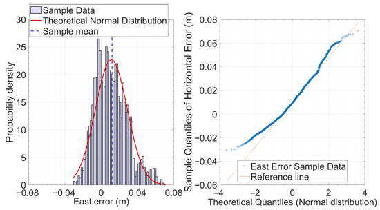
Figure 2.
Normality analysis of the East component of the error in the static test. (Left): histogram of the empirical distribution of the East error (m), overlaid with the theoretical normal density estimated from the data. (Right): QQ-plot comparing the sample quantiles of the East error with the theoretical quantiles of a standardized normal distribution. The tails show clear deviations from normality, with evidence of positive skewness and leptokurtosis, also confirmed by the test of Lilliefors, with p < 0.001.
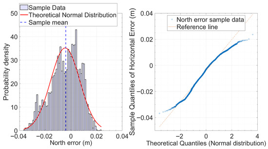
Figure 3.
Normality analysis of the North component of the error in the static test. (Left): histogram of the empirical distribution of the North error (m) with the estimated normal curve (continuous red line) and the sample mean (dashed blue line). (Right): QQ-plot comparing the sample quantiles of the North error with the theoretical quantiles of a standardized normal distribution. The distribution appears more symmetric than the East component, but the normality tests still lead to the rejection of the normality hypothesis (p < 0.001), suggesting the presence of heavier tails than the normal distribution.
Table 2.
Bootstrap estimates for East and North error components: sample statistics, bias correction, and 95% BCa confidence intervals.
The fact that the mean errors in the East and North components differ from zero, with confidence intervals not centered around zero, indicates the presence of a significant systematic error that warrants further analysis. One plausible contributing factor to this anomaly could be the use of velocity values from the Matera station (MATE00ITA) to update the position of the Naples station during the transformation between the ETRF2000 reference frame (epoch 2008.0) and ITRF2020 (current epoch). In fact, an accurate transformation between terrestrial reference frames requires not only the initial coordinates but also station-specific velocity values, to account for tectonic motion and local deformations over time [21]. In the absence of specific velocity data for Naples, the adoption of those from the Matera station, geographically close but geodynamically different, introduces a residual systematic bias in the transformed coordinates. The horizontal error is defined as the Euclidean norm of the 2D vector formed by the East and North components. If these components were independent Gaussian variables with equal variance, the horizontal error would follow a Rayleigh distribution. However, in our dataset, the components deviate from normality, exhibiting noticeable skewness and heavy tails. Therefore, a more robust empirical approach is preferred, using bootstrap techniques and fitting flexible distributions (such as Weibull or Gamma) to model the horizontal error distribution more accurately, derive robust statistics, and construct reliable confidence intervals.
Figure 4 illustrates the distribution of empirical horizontal errors, presented as a histogram with a bin width of 2 mm. The plot includes overlays of the fitted Rayleigh (green) and Weibull (red) distributions, with all distribution parameters estimated directly from the sample data. The horizontal error does not follow the expected Rayleigh distribution (which would be the case for independent and identically distributed (IID) Gaussian East/North components), nor does it match a simple Weibull distribution, due to pronounced skewness and heavy tails. The results of the Kolmogorov–Smirnov test quantitatively support these findings. When testing the fit to a Rayleigh distribution, the p-value is extremely low—approximately zero—which leads to a strong rejection of this model. Although the p-value for the Weibull distribution is somewhat higher, at 0.0050, it still falls below the commonly accepted significance threshold, indicating that this model should also be rejected. These numerical results confirm the visual evidence and non-normality of the East and North components: the horizontal error distribution is heavily skewed and heavy-tailed. Therefore, non-parametric methods, such as bootstrap (applied here in its non-parametric form with bias correction), are necessary for deriving reliable statistics and robust confidence intervals.
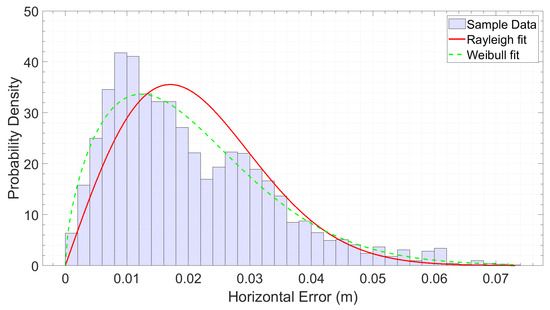
Figure 4.
Empirical distribution of horizontal errors represented by histogram, overlaid with the theoretical Rayleigh (red) and Weibull (green) distributions. The parameters for both Rayleigh and Weibull theoretical curves were estimated directly from the sample data using the MATLAB function fitdist, which fits probability distributions to data by finding the parameter values that best match the sample. Each bin has a width of 2 mm. The differences between the empirical data and the theoretical distributions are clearly visible.
The estimated bootstrap bias is essentially zero for all statistics, indicating that the sample estimates are well-centered and do not require any significant correction. This supports the reliability of the values obtained directly from the data. The mean horizontal error is 0.020 m, with a very narrow confidence interval (0.020–0.021 m), pointing to high consistency. The median is slightly lower, at 0.017 m, which suggests a right-skewed distribution—something also reflected in the gap between the mean and the median. Looking at variability, the standard deviation is 0.013 m, while the median absolute deviation (MAD) is lower, at 0.008 m. This difference implies the presence of some outliers or asymmetry in the data. As expected when extreme values are present, the RMS error is higher than the standard deviation, at 0.024 m. The mean horizontal error around 0.020 m is in line with the stated accuracy of PointPerfect Flex (0.03–0.06 m). Overall, this analysis not only confirms the robustness of the estimates but also offers useful insight into the structure of the errors, which is key for improving high-precision applications. Figure 5 presents a scatter plot of horizontal positioning errors, including the Circular Error Probable at 50% and 95% confidence levels (CEP and CEP95). Since horizontal error is not distributed as Rayleigh, the CEP95 was computed empirically as the 95th percentile of the observed errors. Most error samples are tightly clustered around the true position, with a CEP of 0.017 m and a CEP95 of 0.046 m. The distribution of the errors shows minimal bias and no significant anisotropy, suggesting consistent corrections in both the East and North components.
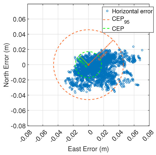
Figure 5.
Horizontal error scatter plot. Each point represents a single horizontal error measurement with respect to the true position. The dashed orange circle denotes the 95% Circular Error Probable (CEP95) with a radius of 0.046 m, while the dashed green circle shows the standard (50%) CEP with a radius of 0.017 m.
The difference between CEP and CEP95 highlights the presence of an error distribution with heavy tails and skewness underscoring the importance of considering both metrics for a comprehensive assessment of accuracy.
Time-Series and Frequency Domain Analysis
For the analysis of errors both in the time and frequency domains, a normalization of the time series was applied by subtracting the estimated mean from each component centering the errors around zero, removing the effect of a constant offset that could negatively influence subsequent analyses.
In Figure 6, the normalized autocorrelation functions of the positioning error time series for the East and North components are shown in panels (a) and (c), respectively. Clearly, both autocorrelations exhibit a sharp peak near zero, followed by a rapid decay. However, a difference between the two components becomes evident at longer time lags. In the East component (panel a), several peaks remain visible beyond 2000 s lags as highlighted by the black dashed ellipse in the figure. In contrast, the North component (panel c) shows a faster decay, and such features are no longer observable. This prolonged persistence in the East suggests the presence of additional periodic or quasi-periodic components, or possibly longer-term correlations. Meanwhile, the North autocorrelation diminishes more quickly, and its periodic structure fades with increasing lag, indicating a stronger influence of white noise and less stable oscillatory behavior. Moreover, in these panels, regular oscillations are visible, suggesting the presence of a periodic component in both error components. To better highlight this periodicity, in panels (b) and (d) zoomed versions of autocorrelation functions centered near 0 are reported for the East and North components, respectively. In these panels, the regular spacing between successive peaks is evident. The overlaid red vertical lines mark intervals of 30, 60, and 90 s better highlight this. The distance between the peaks is consistently 30 s. Thus, we can formulate the hypothesis of a dominant periodic component with a 30 s period in both the East and North GNSS error time series. This motivates a more detailed spectral analysis, presented in the following section, to quantify the dominant frequencies and further characterize the temporal behavior of the GNSS positioning errors.
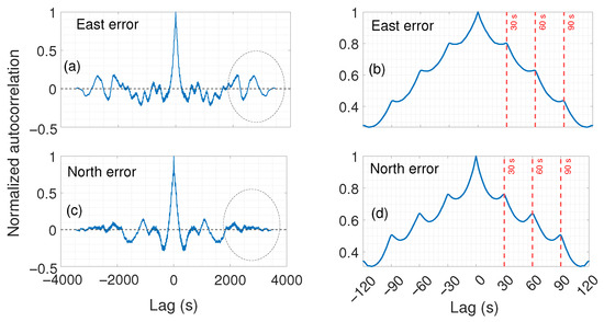
Figure 6.
East and North error autocorrelation. Panel (a) in the upper left shows the autocorrelation function of the East coordinate errors over the full range of lags. Panel (b) in the upper right presents a zoomed-in view of panel (a), focusing on the central lags to highlight the structure of the autocorrelation peaks. The second row displays the corresponding plots for the North coordinate errors: panel (c) shows the full autocorrelation, and panel (d) provides the zoomed-in view. On the zoomed version panel (b,d) are overlapped vertical lines at lags of 30, 60 and 90 s, respectively.
Figure 7 shows the Power Spectral Density (PSD) of the East and North components. PSD was estimated using Welch’s method with a Hanning window of 512 samples, 50% overlap, and a FFT of 1024 points, providing a robust and smooth spectral representation. Given the 1 Hz sampling rate, the Nyquist frequency is 0.5 Hz. In both the East and the North components, besides a peak around 1 mHz, a peak is clearly visible centered at 1/30 Hz (33 mHz) along with the other harmonics at multiples of 1/30 Hz (66 mHz, 99 mHz). This is the evidence of a periodic phenomenon with a 30 s period. To highlight this periodicity, vertical red lines were added at these frequencies.
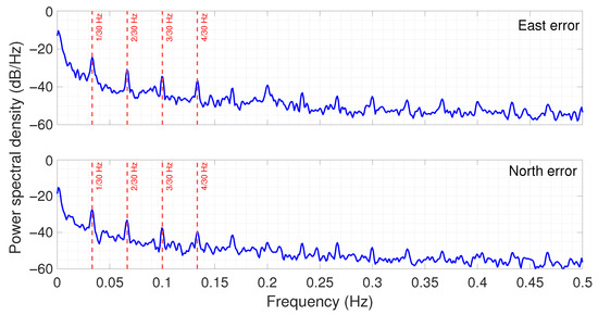
Figure 7.
Power Spectral Density (PSD) of GNSS positioning errors for the East and North components, computed using Welch’s method with a 512-sample Hanning window, 50% overlap, and 1024-point FFT. Vertical lines are overlaid at frequencies corresponding to Hz and its harmonics to highlight the presence of a periodic signal with a 30 s period.
The spectral content outside these peaks is indicative of broadband noise typical of GNSS positioning errors. Notably, the distinct periodic components observed in Figure 7 align closely with the known update interval of atmospheric corrections in the PointPerfect service, pointing to a likely correlation between the correction timing and the observed error structure.
To isolate behaviors at specific moments in time that are not detectable using PSD, we employed Continuous Wavelet Transform (CWT) analysis. This approach allows a signal to be represented in the time-scale domain, by correlating the signal with a function known as the mother wavelet, which is appropriately scaled and translated over time. In particular, the CWT of a signal is defined as the inner product between and the scaled and translated mother wavelet , formally expressed as
where a is the scale parameter (dilation/compression), b is the time translation, and is the complex conjugate of the mother wavelet [28].
This approach allows the analysis of non-stationary signals, characterized by time-varying frequencies, overcoming the limitations of the Fourier Transform which only provides global frequency information. This analysis is especially suitable for signals such as PPP-RTK errors, where one aims to identify temporary events and time-varying frequency components. The scalogram, which visualizes the power of wavelet coefficients over time and period (inverse of frequency), provides an intuitive and detailed representation of the signal’s dynamics.
Figure 8 shows the scalogram obtained by Continuous Wavelet Transform (CWT) using the Morlet wavelet. On the horizontal axis is reported the GPS time expressed in seconds of the week. On the vertical axis is reported the analyzed periods in seconds. The Morlet wavelet was chosen for its joint time–frequency localization properties. The color scale corresponds to wavelet power: blue lines indicate low power, while yellow ones indicate high power at specific times and periods. On the figure, red lines are superimposed to draw the reader’s attention to the periods around 30 s already highlighted in previous findings. However, an intriguing anomaly occurs between 204,300 and 205,300 s, where the North component (upper panel) exhibits a distinct absence of this harmonic.
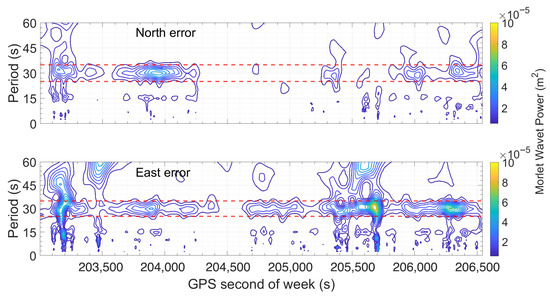
Figure 8.
Scalogram of North (upper box) and East (lower box) errors. The horizontal axis represents GPS time in seconds of the week, while the vertical axis shows the analyzed periods in seconds. The color scale encodes wavelet power, with cooler colors (blue) indicating lower power and warmer colors (yellow) indicating higher power at specific periods and times. Dashed red lines highlight statistically significant periodicities, notably around 30 s, suggesting the presence of persistent oscillatory components in the error signal.
Figure 9 shows the scalogram of the horizontal positioning error, which inherently reflects the combined contributions of both the East and North error components. Upon examination of the scalogram, it is evident that the time interval between 204,000 and 204,800 s of the GPS week exhibits an absence of pronounced error peaks (as already seen, but in a wider interval, for the North component in the previous figure). This observation suggests a period of relative error stability. Consequently, it is of particular interest to focus error analysis in this interval.
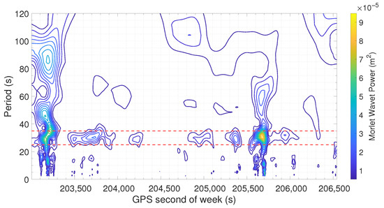
Figure 9.
Scalogram of horizontal errors. The horizontal axis represents GPS time in seconds of the week, while the vertical axis shows the analyzed periods in seconds. The color scale encodes wavelet power, with cooler colors (blue) indicating lower power and warmer colors (yellow) indicating higher power at specific periods and times. Dashed red lines highlight statistically significant periodicities, notably around 30 s, suggesting the presence of persistent oscillatory components in the error signal.
Figure 10 shows the scatter plot along with the CEP and CEP95 for fixed solutions in the time span from [240,000–240,800 s], when the 30 s period component is not present. In this interval, we observe a significant improvement, with both CEP and CEP95 reduced by half, namely the CEP reaches 0.01 m while the CEP95 reaches 0.019 m. This result is confirmed by the statistics shown in Table 3, which summarizes the descriptive statistics—including the mean, standard deviation, median, MAD, RMS—calculated from the sample data in the selected time interval. Also for this sample, to improve estimator reliability, bootstrap resampling was applied to evaluate bias and construct 95% bias-corrected and accelerated (BCa) confidence intervals. The bias estimates are minimal across all metrics, indicating negligible skewness in the error distributions. The mean error is 0.010 m with a narrow confidence interval [0.010, 0.011 m], confirming a consistent low error during this interval. Both the standard deviation and median values show a low dispersion (0.005 m and 0.010 m, respectively), while robust measures such as MAD (0.003 m) and RMS (0.011 m) confirm the low horizontal error. These results validate the scalogram’s identification of time periods characterized by minimal horizontal positioning error.
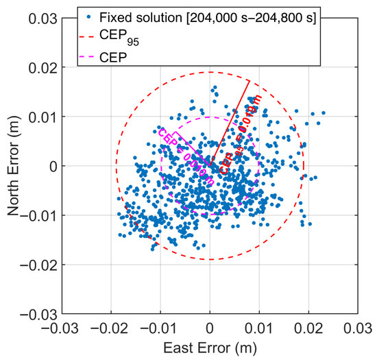
Figure 10.
Horizontal error scatter plot during time span from [204,000–204,800 s] when 30 s period components is not present. Each point represents a single horizontal error measurement with respect to the true position. The dashed orange circle denotes the 95% Circular Error Probable (CEP95) with a radius of 0.019 m, while the dashed green circle shows the standard (50%) CEP with a radius of 0.01 m.
Table 3.
Bootstrap analysis with bias correction and 95% BCa confidence intervals for horizontal error between 204,000 and 204,800 s.
4. Performance Comparison with Previous Service
To assess the evolution of the correction service’s performance, a comparative analysis was conducted using a dataset collected on 2 January 2023, when an earlier version of PointPerfect was in use. The goal was to evaluate whether the current version of the service demonstrates improvements in terms of positioning accuracy.
The results of the BCa bootstrap analysis, including bias-corrected 95% confidence intervals for this dataset, are reported in Table 4. Comparison reveals that these results and those obtained with PointPerfect flex correction (Table 2 and Table 5) clearly shows that the new PointPerfect method significantly improves over the traditional approach. The East component’s RMS error decreases from 0.057 m (traditional) to 0.021 m (new flex service), and the North component’s RMS drops from 0.056 m to 0.012 m, while the mean shrinks from −0.05 m to 0.012 m. Similar improvements are seen in MAD and median values, confirming more stable and reliable estimates. Overall, these results demonstrate the enhanced accuracy and robustness of the new algorithm, especially in horizontal positioning metrics. To provide a clear and immediate visual comparison, a boxplot is shown in Figure 11, presenting a comparative analysis of positioning errors in the East, North, and horizontal components using both the previous and current PointPerfect correction services. Each boxplot displays the median (red line), interquartile range (blue box), whiskers (black lines indicating the range within 1.5 times the interquartile range), and outliers (red crosses). Superimposed light blue rectangles represent the 95% confidence intervals of the medians, estimated using the BCa bootstrap method. These intervals are barely visible due to their narrow width, reflecting the high precision and statistical reliability of the median estimates. When comparing the two services, a notable improvement in positioning performance is observed with the current correction. In the East component, the current correction significantly reduces both the bias and variability of the errors. The median is closer to zero, and the interquartile range is narrower, indicating increased accuracy and precision. Additionally, the number and magnitude of outliers are reduced. In the North component, both corrections yield medians close to zero and relatively tight distributions; however, the current correction further improves precision with a slightly more compact interquartile range and fewer extreme values. The most substantial improvement is observed in the horizontal error component, which combines East and North errors. The distribution under the current correction is markedly narrower, with a lower median and fewer outliers, demonstrating enhanced overall positioning consistency.
Table 4.
Bootstrap analysis with bias correction and 95% BCa confidence intervals for East, North and horizontal components of 2 January 2023 data collection.
Table 5.
Bootstrap analysis with bias correction and 95% BCa confidence intervals for horizontal error.
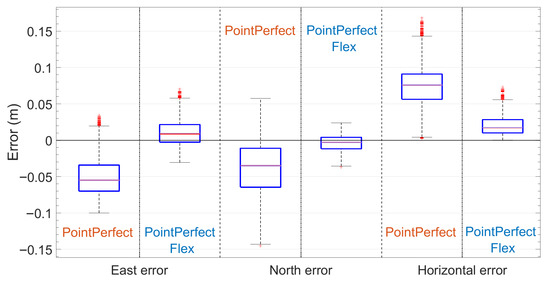
Figure 11.
Box plots comparison of positioning errors in the East, North and horizontal component for current and previous PointPerfect correction service. Each box shows the median (red line), quartiles (horizontal blue lines), whiskers (horizontal black lines), and possible outliers (red crosses) distribution of errors allowing a fast comparison. Light blue rectangles superimposed on each box represent the 95% confidence intervals of the median.
To effectively compare the accuracies and precisions reachable by using the two distinct services, the error scatter plot is shown in Figure 12. The plot displays individual error samples as blue (PointPerfect Flex) and orange (PointPerfect) dots. The 95% Circular Error Probable (CEP95) is depicted for each solution as dashed circles. The PointPerfect Flex solution exhibits a substantially smaller and more concentrated error distribution compared to PointPerfect, as evidenced by the smaller CEP95 circle—reduced from 0.1242 m with the standard PointPerfect configuration to 0.044 m with PointPerfect Flex. The figure also clearly highlights the improvement in precision: the blue dots are significantly more clustered than the orange ones, reflecting a reduction in the standard deviation of the horizontal error from 0.030 m to 0.013 m—approximately a one-third decrease. This demonstrates the superior horizontal accuracy and consistency of PointPerfect Flex.
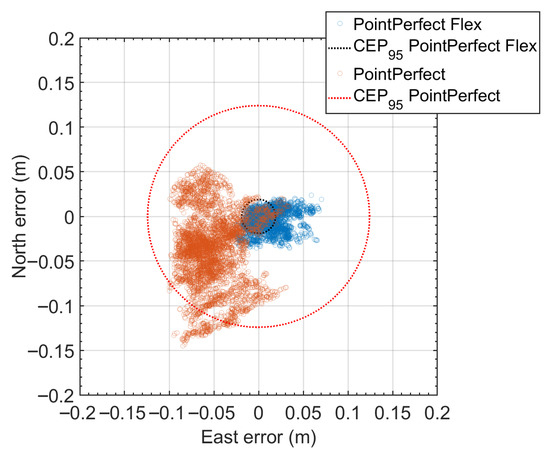
Figure 12.
Horizontal error scatter plot during the data collection of 2 January. Each point represents a single horizontal error measurement with respect to the true position. The red dots correspond to the results obtained on 2 January, while the blue dots represent those from 6 June. The two circles indicate the CEP95 values, with a radius of 0.1242 m for the old PointPerfect correction and 0.046 m for the new version.
To further investigate the comparison, a time–frequency analysis was performed using the Morlet wavelet in Figure 13. By comparing Figure 13 with Figure 9 it can be noted that also in the older dataset around the 30 s period band (33 mHz) a persistent energy concentration is present. The difference is that in older PointPerfect, the energy is present across extended time intervals suggesting a less effective compensation of short-period errors in the previous implementation. By comparing Figure 13 with Figure 9, it can be noted that the difference is that in the older PointPerfect implementation, the energy is distributed across extended time intervals, suggesting a less effective compensation of short-period errors. A different color scale was employed here, with a higher value of energy associated to yellow, to account for the higher noise level in the data collected on 2 January 2023. Despite the general improvement observed with the new service, it is important to note that the 33 mHz component is not entirely absent. While significantly reduced in magnitude and temporal persistence, faint traces of this frequency band still appear in Figure 9, particularly near the prominent peaks around GPS seconds 203,500 and 205,500. This indicates that the 30 s oscillatory component remains a residual feature of the error process. The analysis presented in this study confirms that centimeter-level positioning accuracy is achievable using low-cost GNSS hardware when augmented with a commercial PPP-RTK correction service such as u-blox PointPerfect. Under quasi-open-sky static conditions, the mean horizontal error of 0.02 m and a CEP95 of 0.046 m are fully aligned with the expected performance of the correction service, validating its reliability for high-precision applications. While mean errors in both the East and North components were statistically significant, they may not represent persistent systematic biases and should be interpreted cautiously. One plausible contributing factor is the use of non-local velocity data during the reference frame transformation, which may introduce small residual shifts. The use of bias-corrected and accelerated (BCa) bootstrap methods provided a robust statistical characterization of the positioning errors. These methods provided accurate confidence intervals for key metrics such as mean error, RMS, and median absolute deviation (MAD), even in the presence of non-Gaussian error. However, a key finding of this study is the detection of a dominant 33 mHz harmonic in the positioning error, corresponding to the 30 s update rate of atmospheric corrections in the PointPerfect service for both the new and old versions. Wavelet scalograms allowed a detailed exploration of these time-varying periodicities, identifying intervals where the 30 s oscillation was absent or diminished. Within these “quiet” periods, horizontal positioning error decreased markedly, with the CEP95 dropping to 0.019 m and the RMS falling to 0.011 m. These findings suggest that both correction update timing and environmental stability can significantly influence PPP-RTK performance.
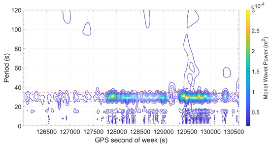
Figure 13.
Scalogram of horizontal errors for the dataset of 2023. The horizontal axis represents GPS time in seconds of the week, while the vertical axis shows the analyzed periods in seconds. The color scale encodes wavelet power, with cooler colors (blue) indicating lower power and warmer colors (yellow) indicating higher power at specific periods and times. Dashed red lines highlight statistically significant periodicities, notably around 30 s, suggesting the presence of persistent oscillatory components in the error signal.
5. Conclusions and Future Work
This study has provided a detailed characterization of positioning errors from a low-cost GNSS receiver (u-blox ZED-F9P) using the PointPerfect PPP-RTK correction service under static, quasi-open-sky conditions. The system consistently achieved centimeter-level horizontal errors, with a mean of approximately 0.02 m and a CEP95 of 0.046 m, confirming the declared performance of the correction service. The use of BCa bootstrap methods enabled statistically robust estimation of error metrics, accounting for the observed non-Gaussianity and asymmetries in the error distributions. Spectral and wavelet analyses revealed a dominant 33 mHz harmonic, corresponding to the 30 s update interval of atmospheric corrections. This periodic component, embedded within the correction stream, introduces consistent temporal structures in the positioning error. Wavelet scalograms further highlighted specific time intervals where the spectral energy at 33 mHz was notably reduced; during these intervals, positioning performance improved significantly, with RMS errors as low as 0.011 m and CEP95 reaching 0.019 m. These observations underscore the temporal variability in correction quality and its measurable impact on positioning accuracy.
A clear improvement in horizontal positioning performance has been observed when comparing the legacy PointPerfect service with the updated PointPerfect Flex. Under static conditions, the mean horizontal error decreased from approximately 0.042 m with the older service to 0.020 m with the new one. Similarly, the 95% Circular Error Probable (CEP95) was significantly reduced, passing from 0.1242 m to 0.046 m. This improvement is also reflected in the precision of the solutions: the standard deviation of the horizontal error was reduced from 0.030 m to 0.013 m, corresponding to a reduction of more than 50%. Furthermore, a time–frequency analysis using the Morlet wavelet revealed that while both solutions exhibit energy concentrations around the 30 s period band (33 mHz), the legacy service shows broader and more persistent patterns over time. This suggests that the updated correction model more effectively mitigates short-period error components, likely due to the introduction of localized, position-aware corrections. The findings emphasize the importance of a multi-domain analytical approach for evaluating PPP-RTK performance, particularly when using low-cost GNSS hardware. Future research will extend this methodology to real-time and kinematic scenarios and explore adaptive filtering techniques to mitigate the periodic error component at around 33 mHz, aiming to evaluate the robustness of the results under varying multipath conditions and atmospheric effects, with the goal of enhancing measurement stability and reducing residual periodic errors.
Author Contributions
Conceptualization, U.R., M.C. and G.P.; methodology, U.R., M.C. and G.P.; software, U.R., M.C. and G.P.; validation, U.R., M.C. and G.P.; formal analysis, U.R., M.C. and G.P.; investigation, U.R., M.C. and G.P.; resources, U.R., M.C. and G.P.; data curation, U.R., M.C. and G.P.; writing—original draft preparation, U.R., M.C. and G.P.; writing—review and editing, U.R., M.C. and G.P.; visualization, U.R., M.C. and G.P.; supervision, U.R., M.C. and G.P.; project administration, U.R., M.C. and G.P.; funding acquisition, U.R. All authors have read and agreed to the published version of the manuscript.
Funding
This research and the APC were funded by the PRIN 2022 Research Project “NAvigation TO GO (NATOGO)”—CUP I53D23006510001.
Data Availability Statement
The raw data supporting the conclusions of this article will be made available by the authors on request.
Conflicts of Interest
The authors declare no conflicts of interest.
Abbreviations
The following abbreviations are used in this manuscript:
| BCa | Bias-Corrected and Accelerated (bootstrap method) |
| CEP/CEP95 | Circular Error Probable (50%/95%) |
| CLAS | Centimeter-Level Augmentation Service |
| CSSR | Compact State Space Representation |
| CWT | Continuous Wavelet Transform |
| ECTT | ETRF/ITRF Coordinate Transformation Tool |
| EPN | EUREF Permanent GNSS Network |
| ETRF | European Terrestrial Reference Frame |
| ETRS | European Terrestrial Reference System |
| FFT | Fast Fourier Transform |
| GNSS | Global Navigation Satellite System |
| HAS | High-Accuracy Service |
| HPAC | High-Precision Atmosphere Correction |
| IGS | International GNSS Service |
| IP | Internet Protocol |
| IoT | Internet of Things |
| ITRF | International Terrestrial Reference Frame |
| MAD | Median Absolute Deviation |
| MQTT | Message Queuing Telemetry Transport |
| NRTK | Network Real-Time Kinematic |
| OCB | Orbit, Clock, Bias |
| PPP-RTK | Precise Point Positioning Real-Time Kinematic |
| PSD | Power Spectral Density |
| QZSS | Quasi-Zenith Satellite System |
| RINEX | Receiver Independent Exchange Format |
| RMS | Root Mean Square |
| RTCM | Radio Technical Commission for Maritime Services |
| RTK | Real-Time Kinematic |
| SPARTN | Secure Position Augmentation for Real-Time Navigation |
| SSR | State Space Representation |
References
- Teunissen, P.; Montenbruck, O. Springer Handbook of Global Navigation Satellite Systems; Springer: Berlin/Heidelberg, Germany, 2017; Volume 10. [Google Scholar] [CrossRef]
- Alkan, R.M.; Erol, S.; İlçi, V.; Ozulu, İ.M. Comparative analysis of real-time kinematic and PPP techniques in dynamic environment. Measurement 2020, 163, 107995. [Google Scholar] [CrossRef]
- Gurtner, W.; Estey, L. Rinex–The Receiver Independent Exchange Format-Version 3.00; Astronomical Institute, University of Bern and UNAVCO: Bolulder, CO, USA, 2007. [Google Scholar]
- Heo, Y.; Yan, T.; Lim, S.; Rizos, C. International standard GNSS real-time data formats and protocols. In Proceedings of the IGNSS Symposium 2009, Surfers Paradise, Australia, 1–3 December 2009. [Google Scholar]
- Vana, S.; Aggrey, J.; Bisnath, S.; Leandro, R.; Urquhart, L.; Gonzalez, P. Analysis of GNSS correction data standards for the automotive market. Navigation 2019, 66, 577–592. [Google Scholar] [CrossRef]
- Ansari, K.; Corumluoglu, O.; Verma, P.; Pavelyev, V.S. An overview of the international GNSS service (IGS). Grenze Int. J. Comput. Theory Eng. 2017. [Google Scholar] [CrossRef]
- QZSS System Service Inc. Centimeter Level Augmentation Service (CLAS). 2020. Available online: https://qzss.go.jp/en/overview/services/sv06_clas.html (accessed on 10 October 2025).
- Savchuk, S.; Grzegorzewski, M.J.; Gołda, P.; Kerker, V. Positioning using the precision Galileo has service. Annu. Navig. 2024, 29. [Google Scholar] [CrossRef]
- Naciri, N.; Yi, D.; Bisnath, S.; de Blas, F.J.; Capua, R. Assessment of Galileo High Accuracy Service (HAS) test signals and preliminary positioning performance. GPS Solut. 2023, 27, 73. [Google Scholar] [CrossRef] [PubMed]
- Trimble. Trimble Website. 2025. Available online: https://positioningservices.trimble.com/services/rtx/ (accessed on 6 August 2025).
- NovAtel Inc. TerraStar-X Corrections Service. 2024. Available online: https://terrastar.net/ (accessed on 10 October 2025).
- U-blox. U-Blox PointPerfect Flex Webpage. 2025. Available online: https://www.u-blox.com/en/product/pointperfectflex (accessed on 2 May 2025).
- Teria. TeriaSat: La Correction Centimétrique Partout en France. 2024. Available online: https://www.reseau-teria.com/teriasat/ (accessed on 2 May 2025).
- Swift Navigation Inc. Skylark GNSS Cloud Corrections. 2023. Available online: https://www.swiftnav.com/skylark/ (accessed on 3 May 2025).
- Geoscience Australia and LINZ. SouthPAN: Southern Positioning Augmentation Network. 2022. Available online: https://www.ga.gov.au/southpan (accessed on 3 May 2025).
- U-blox. U-Blox ANN-MB Antenna Data Sheet. 2022. Available online: https://content.u-blox.com/sites/default/files/ANN-MB_ProductSummary_UBX-18047741.pdf (accessed on 16 September 2022).
- Robustelli, U.; Cutugno, M.; Paziewski, J.; Pugliano, G. GNSS-SDR pseudorange quality and single point positioning performance assessment. Appl. Geomat. 2023, 15, 583–594. [Google Scholar] [CrossRef]
- Robustelli, U.; Cutugno, M.; Pugliano, G. Low-Cost GNSS and PPP-RTK: Investigating the Capabilities of the u-blox ZED-F9P Module. Sensors 2023, 23, 6074. [Google Scholar] [CrossRef] [PubMed]
- Amalfitano, D.; Cutugno, M.; Robustelli, U.; Pugliano, G. Designing and Testing an IoT low-cost PPP-RTK augmented GNSS Location device. Sensors 2024, 24, 646. [Google Scholar] [CrossRef] [PubMed]
- Ferguson, K.; Urquhart, L.; Leandro, R. SPARTN: The First Open GNSS Data Standard that Enables Safe and Accurate GNSS Localization for Automotive Applications. In Proceedings of the 33rd International Technical Meeting of the Satellite Division of the Institute of Navigation (ION GNSS+ 2020), Virtual, 21–25 September 2020; pp. 2092–2106. [Google Scholar]
- EUREF. ETRF/ITRF Coordinate Transformation Tool (ECTT). 2022. Available online: https://epncb.oma.be/_productsservices/coord_trans/ (accessed on 19 October 2025).
- Lilliefors, H.W. On the Kolmogorov-Smirnov test for normality with mean and variance unknown. J. Am. Stat. Assoc. 1967, 62, 399–402. [Google Scholar] [CrossRef]
- Dallal, G.E.; Wilkinson, L. An analytic approximation to the distribution of Lilliefors’s test statistic for normality. Am. Stat. 1986, 40, 294–296. [Google Scholar] [CrossRef]
- Efron, B.; Tibshirani, R.J. An Introduction to the Bootstrap. In Monographs on Statistics and Applied Probability; Chapman & Hall/CRC: New York, NY, USA, 1993; Volume 57. [Google Scholar]
- Efron, B.; DiCiccio, T. Bootstrap Confidence Intervals. Stat. Sci. 1996, 11, 189–228. [Google Scholar] [CrossRef]
- Davison, A.C.; Hinkley, D.V. Bootstrap Methods and Their Application; Cambridge Series in Statistical and Probabilistic Mathematics; Cambridge University Press: Cambridge, UK, 1997; Volume 1. [Google Scholar]
- Cressie, N.; Wikle, C.K. Statistics for Spatio-Temporal Data; John Wiley & Sons: Hoboken, NJ, USA, 2011. [Google Scholar]
- Pugliano, G.; Robustelli, U.; Santamaria, R. A new method for specular and diffuse pseudorange multipath error extraction using wavelet analysis. GPS Solut. 2016, 20, 499–508. [Google Scholar] [CrossRef]


Disclaimer/Publisher’s Note: The statements, opinions and data contained in all publications are solely those of the individual author(s) and contributor(s) and not of MDPI and/or the editor(s). MDPI and/or the editor(s) disclaim responsibility for any injury to people or property resulting from any ideas, methods, instructions or products referred to in the content. |
© 2025 by the authors. Licensee MDPI, Basel, Switzerland. This article is an open access article distributed under the terms and conditions of the Creative Commons Attribution (CC BY) license.