WSG-FEC: Gray-Box Frequency-Domain Explanation of CNN Models Based on Weakly Supervised Learning

Abstract

Convolutional neural networks (CNNs) have achieved remarkable progress in recent years, largely driven by advances in computational hardware. However, their increasingly complex architectures continue to pose significant challenges for interpretability. Existing explanation methods predominantly rely on spatial saliency representations and therefore fail to capture the intrinsic frequency-domain characteristics of image data. This work introduces WSG-FEC, a Weakly Supervised Gray-box Frequency-domain Explanation framework that integrates multilevel Haar wavelet decomposition with gradient-weighted class activation mapping (Grad-CAM) to generate frequency-aware explanations. By leveraging hierarchical wavelet structures, the proposed method produces frequential–spatial saliency maps that overcome the low-resolution limitations of white-box approaches and the high computational cost of black-box perturbation methods. Quantitative evaluations using insertion and deletion metrics demonstrate that WSG-FEC provides more detailed, efficient, and interpretable explanations, offering a novel perspective for understanding CNN decision mechanisms.

1. Introduction

Convolutional neural networks (CNNs) play a central role in modern computer vision, yet their increasing architectural complexity and nonlinear behavior make them inherently difficult to interpret. As CNNs continue to evolve, understanding their internal reasoning becomes increasingly important for both transparency and reliability, especially in high-stakes applications, such as medical diagnosis, remote sensing interpretation, industrial defect inspection, and autonomous driving [1]. Compared with traditional machine learning models, CNNs operate as highly opaque systems, motivating the development of effective explanation techniquess [2].

Existing explainability methods for CNNs can be broadly categorized into white-box and black-box approaches. White-box methods, such as CAM [3] and its variants Grad-CAM [4] and Grad-CAM++ [5], compute class-specific weights for feature maps and generate coarse activation maps with relatively low computational cost. However, their spatial resolution decreases significantly as network depth increases. Other white-box strategies include self-explainable architectures such as ProtoPNet [6], Semi-ProtoPNet [7], PS-ProtoPNet [8], and Comb-ProtoPNet [9], which embed prototype-based reasoning into the model design.

Black-box methods, including RISE [10], GSM-HM [11], Occlusion [12], and LIME [13], rely on perturbation-based sampling to approximate model behavior. These approaches typically produce higher-resolution explanations but require substantial computational resources due to repeated inference.

Despite these advances, most existing methods focus exclusively on spatial representations and overlook the frequency-domain properties inherent in digital images. Prior studies have shown that high-frequency components often play a critical role in CNN performance [14], and small perturbations in wavelet coefficients can produce disproportionately large effects on model outputs. These observations suggest that frequency-domain analysis may offer a more informative and efficient pathway for interpretability.

Based on these observations, a hierarchical method is proposed that uses a multilevel wavelet decomposition of the original image data to obtain explanations with reduced computational cost from an innovative frequency domain perspective. The framework integrates wavelet frequency hierarchies with CAM, using it as a weakly supervised label, and refines the technique through a random optimization process. These steps effectively address the resolution limitations of white box methods and the computational demands of black box approaches while improving output interpretability by combining both methodologies into a gray box approach. The study methodology improves saliency map generation and produces unique visualization results in explainable artificial intelligence (XAI), setting a new benchmark for future research.

To overcome the limitations of existing explanation methods, this study proposes a Weakly Supervised Gray-box Frequency-domain Explanation framework (WSG-FEC). By combining multilevel Haar wavelet decomposition with Grad-CAM heatmaps, the framework generates explanations from a frequency-domain perspective, achieving a balance between efficiency and resolution. The objectives of this research are:

• To provide an explanation method that simultaneously ensures computational efficiency and interpretive accuracy;
• To explore the role of frequency-domain features in enhancing CNN interpretability;
• To establish a multi-level explanation framework that reveals the model’s recognition ability at different frequency scales.

This study not only enriches the theoretical perspective of explainable artificial intelligence but also offers practical interpretability tools for applications such as medical imaging, remote sensing, and industrial inspection.

2. Related Work

2.1. Frequency-Domain Observations of CNN Models

Digital images naturally contain frequency-domain information, and convolutional operations correspond to multiplication in the frequency domain. Consequently, analyzing CNNs from a frequency perspective is both intuitive and theoretically grounded [15,16,17]. Prior work has demonstrated the benefits of frequency-based representations: for example, Chęciński et al. [18] showed that optimizing discrete cosine transform (DCT) parameters can be more efficient than directly training convolutional filters. Lin et al. [19] introduced feature pyramid networks (FPNs), highlighting the importance of combining coarse and fine features across scales. Zhang et al. [20] further observed that CNNs gradually shift their frequency response from low to high frequencies during training, improving generalization.

These findings collectively suggest that frequency-domain analysis may provide valuable insights into CNN behavior, motivating the present study.

2.2. White-Box Explanation Methods

White-box methods leverage internal model information to generate explanations. CAM [3]-based approaches compute weighted sums of feature maps, where the weights are derived either from global average pooling (GAP) or from gradients. Although computationally efficient, these methods suffer from low spatial resolution, especially in deeper networks. Grad-CAM [4] eliminates the need for retraining by using gradients as weights, while Grad-CAM++ [5] incorporates higher-order derivatives to improve localization accuracy.

Figure 1 illustrates the CAM workflow: GAP is inserted before the classification layer, the fully connected layer is retrained, and class activation maps are obtained by weighting the final convolutional feature maps. Despite their efficiency, CAM-based methods typically produce explanations that are significantly lower in resolution than the original input.

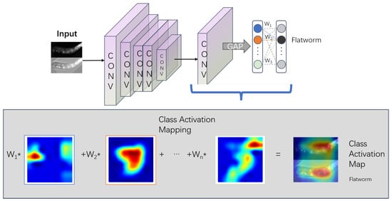
Figure 1. Framework of the CAM method: As shown in the figure, after the final convolutional layer, a GAP is set, and then the FC layer is applied. The class activation for the Australian terrier class equals the sum of each weighted feature map using weight $w_n$. In the figure, the asterisk denotes multiplication.

2.3. Black Box Explanation Methods

Black box methods for interpreting CNNs include occlusion-based approaches, random masking strategies, and surrogate modeling using interpretable models to approximate the target model. Among these, the LIME and RISE methods have significantly inspired the present approach. Both are perturbation-based local explanation techniques that share conceptual similarities with the study methodology. A detailed introduction to them is provided below.

2.3.1. The LIME Method

LIME [13] is a classical black box method that employs a simple, interpretable model to locally approximate the behavior of a complex model through perturbations. This approach is generally effective because global explanations are often inaccessible and unnecessary. The computational complexity of the LIME method increases with the degree of nonlinearity in the target model. The LIME method begins by selecting a complex model that requires interpretation. It then generates samples in the vicinity of the original data and uses the complex model to make predictions on these new samples. Each sample is weighted based on its similarity to the original input, and these weighted samples are used to train a simpler, interpretable model. Finally, the parameters of this simpler model are analyzed to provide insights into the behavior of the original complex model.

2.3.2. The RISE Method

RISE [10], derived from the LIME method, performs local explanations by aggregating weighted perturbation samples directly, without using surrogate modeling. The workflow of the RISE method is presented as follows: Binary masks of a specified size, such as $7\times 7$, were first generated with equal probabilities assigned to 0 and 1. These masks were then upsampled to a higher resolution using bilinear interpolation, followed by random cropping to align with the dimensions of the input image. The resulting masks were applied to the input images through pixelwise multiplication using the Hadamard product. Cosine similarity was computed between the predictions of the masked and original images to assess their alignment. This entire process was iterated N times (for example, 4000 iterations) and the final saliency map was obtained by linearly aggregating the masks, each weighted according to its corresponding similarity score.

In summary, existing explanation methods for CNNs can be broadly divided into white-box and black-box approaches. White-box methods, such as CAM and its variants, are computationally efficient but suffer from low spatial resolution. Black-box methods, such as LIME and RISE, provide higher-resolution explanations but incur significant computational costs due to extensive perturbation sampling. Although some studies have explored frequency-domain perspectives, these efforts remain fragmented and lack a systematic framework for interpretability. Consequently, current approaches fail to simultaneously achieve high efficiency and fine-grained resolution, and they do not fully exploit the intrinsic frequency characteristics of digital images. To address this gap, the present study introduces the WSG-FEC framework, which leverages multilevel wavelet decomposition and weakly supervised learning to provide hierarchical frequency-domain explanations with improved efficiency and accuracy.

3. Gray Box Frequency-Domain Explanation of CNN Models Based on Weakly Supervised Learning

The algorithmic design in Figure 2 of this study is based on the following engineering and theoretical principles: the sparsity of coefficients in digital wavelet decomposition and its effectiveness in texture representation; the coarse-grained nature of Grad-CAM-based outputs; the selection of appropriate explainers; and the choice of suitable optimization strategies. Each of these elements is described in detail in subsections of this part.

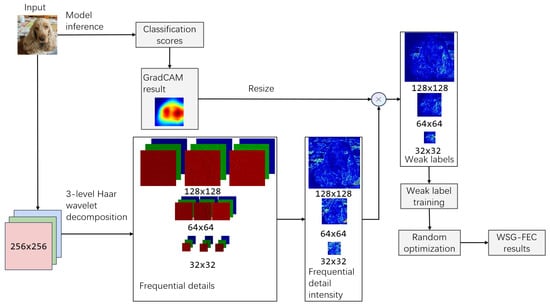
Figure 2. WSG-FEC methodology: The input image undergoes model inference to obtain class scores, followed by rescaled CAM outputs serving as spatial weights in Haar wavelet layers to generate weak labels. These labels are fitted with an autoencoder and refined through randomized optimization, yielding a three-level frequency-based explanation.

3.1. Haar Wavelet Decomposition

The wavelet transform is a classical frequency domain technique in image processing and is widely used in tasks such as edge detection, denoising [21], multiscale analysis, image compression, and image encoding. In digital image applications, Haar wavelet decomposition [22] is particularly advantageous due to its computational simplicity, making it suitable for image encoding and transmission [23]. In this work, three-level Haar wavelet decomposition forms the structural basis of the proposed explanation framework. Only the decomposition phase is used.

A one-dimensional Haar wavelet transform works on vectors with lengths that are powers of 2.

$$whenVector[a,b,c,d]=[1,2,3,4],$$

(1)

Elements are grouped into pairs, and for each pair, the average and the difference are computed to obtain the approximation coefficients and detail coefficients, respectively. All the approximation coefficients are then concatenated to form the approximation vector, and all the detail coefficients form the detail vector. Each vector result is half the length of the original input.

$$Approximation=[{\displaystyle \frac{a+b}{2}},{\displaystyle \frac{c+d}{2}}]=[1.5,3.5],$$

(2)

$$detail=[{\displaystyle \frac{a-b}{2}},{\displaystyle \frac{c-d}{2}}]=[-0.5,-0.5],$$

(3)

$$decompsition=[1.5,3.5,-0.5,-0.5],$$

(4)

Single-level decomposition is presented above; if the approximation is decomposed recursively, it results in a multilevel Haar wavelet decomposition.

Similarly, two-dimensional Haar decomposition follows a similar principle and is mathematically equivalent to applying one-dimensional Haar decomposition sequentially to each row and column of the image matrix.

$$whenVector=\left[\begin{array}{cccc}1& 2& 3& 4\\ 5& 6& 7& 8\\ 9& 10& 11& 12\\ 13& 14& 15& 16\end{array}\right],$$

(5)

After horizontal decomposition:

$$\left[\begin{array}{cccc}{\displaystyle \frac{1+2}{2}}& {\displaystyle \frac{3+4}{2}}& {\displaystyle \frac{1-2}{2}}& {\displaystyle \frac{3-4}{2}}\\ {\displaystyle \frac{5+6}{2}}& {\displaystyle \frac{7+8}{2}}& {\displaystyle \frac{5-6}{2}}& {\displaystyle \frac{7-8}{2}}\\ {\displaystyle \frac{9+10}{2}}& {\displaystyle \frac{11+12}{2}}& {\displaystyle \frac{9-10}{2}}& {\displaystyle \frac{11-12}{2}}\\ {\displaystyle \frac{13+14}{2}}& {\displaystyle \frac{15+16}{2}}& {\displaystyle \frac{13-14}{2}}& {\displaystyle \frac{15-16}{2}}\end{array}\right]=\left[\begin{array}{cccc}1.5& 3.5& -0.5& -0.5\\ 5.5& 7.5& -0.5& -0.5\\ 9.5& 11.5& -0.5& -0.5\\ 13.5& 15.5& -0.5& -0.5\end{array}\right],$$

(6)

After vertical decomposition:   

$$\left[\begin{array}{cccc}{\displaystyle \frac{1.5+5.5}{2}}& {\displaystyle \frac{3.5+7.5}{2}}& {\displaystyle \frac{-0.5-0.5}{2}}& {\displaystyle \frac{-0.5-0.5}{2}}\\ {\displaystyle \frac{9.5+13.5}{2}}& {\displaystyle \frac{11.5+15.5}{2}}& {\displaystyle \frac{-0.5-0.5}{2}}& {\displaystyle \frac{-0.5-0.5}{2}}\\ {\displaystyle \frac{1.5-5.5}{2}}& {\displaystyle \frac{3.5-7.5}{2}}& {\displaystyle \frac{-0.5+0.5}{2}}& {\displaystyle \frac{-0.5+0.5}{2}}\\ {\displaystyle \frac{9.5-13.5}{2}}& {\displaystyle \frac{11.5-15.5}{2}}& {\displaystyle \frac{-0.5+0.5}{2}}& {\displaystyle \frac{-0.5+0.5}{2}}\end{array}\right]=\left[\begin{array}{cccc}3.5& 5.5& -0.5& -0.5\\ 11.5& 13.5& -0.5& -0.5\\ -2& -2& 0& 0\\ -2& -2& 0& 0\end{array}\right]$$

(7)

Similarly, the submatrix composed of the four top-left coefficients after single-level decomposition can be further recursively decomposed using the two-dimensional Haar wavelet transform.

3.2. Quarter Information Test

Three-level Haar decomposition produces one approximation matrix and three detail matrices. The approximation coefficients retain progressively smaller fractions of the original information (1/4, 1/16, and 1/64). To assess their representational fidelity, each approximation is reconstructed into an image and compared with the original using similarity scores. Plotting information quantity against similarity yields the Quarter Information Test (QIT), which serves as a baseline for evaluating the quality of frequency-domain representations.

By plotting the quantity of information against the similarity score, as illustrated in Figure 3, a reference curve called the quarter information test (QIT) is created. This baseline accurately reflects the fidelity of the approximations and serves as a clear criterion for assessing the quality of the representation. At each quarter-information level, only the approximations located in the upper-left region of Figure 3 are tested.

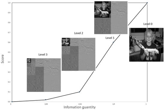
Figure 3. QIT process: The figure shows the original grayscale image and results of three-level 2D wavelet decomposition. Approximation coefficients appear in the upper-left, detail coefficients in the lower-right, with both shrinking in size at each level.

3.3. Autoencoder Explainer

Autoencoders are widely used in tasks such as object recognition, intrusion detection [24], and fault diagnosis [25]. A typical autoencoder consists of an encoder and a decoder: the encoder compresses the input into a low-dimensional representation, whereas the decoder reconstructs it to the original input dimensions. In the study explanation task, the input and output share the same resolution; because both are two-dimensional images, a convolutional autoencoder architecture is particularly well suited to serve as an explainer in this context.

The input to the autoencoder is the frequency-domain detail intensity, as illustrated in Figure 2. Specifically, for each spatial pixel within a given frequency layer, the frequency intensity is defined as the maximum absolute value among all detail coefficients across all color channels and directional components. Let $D_{c,d}^{\left(l\right)}(x,y)$ represent the detail coefficient at level l, color channel $c\in \{R,G,B\}$, and direction $d\in \{\mathrm{horizontal},\mathrm{vertical},\mathrm{diagonal}\}$ at spatial location $(x,y)$. The frequency intensity $F^{\left(l\right)}(x,y)$ used as the input to the autoencoder is defined as follows:

$$F^{\left(l\right)}(x,y)=\underset{c,d}{max}\left|D_{c,d}^{\left(l\right)}(x,y)\right|$$

(8)

In autoencoders based on convolutional neural networks, the encoder consists of several layers of convolutional neurons, whereas the decoder uses 2D transposed convolution units to restore the data dimensions. Detailed information regarding the explainer’s training process is provided in the subsequent subsections.

The structure of the explainer is shown in Figure 4.

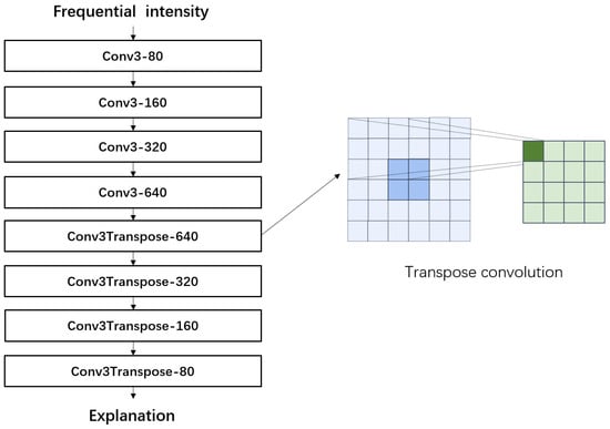
Figure 4. Structure of the autoencoder explainer.

3.4. Weakly Supervised Labels

The study approach involves a frequency-based explanation that uses weakly supervised learning, a machine learning technique that has been widely applied and developed in recent years [26,27,28]. Using Haar wavelet decomposition, explanations and weak labels are derived across three wavelet frequency levels. After performing three-scale two-dimensional wavelet decomposition for each RGB image color channel, three wavelet detail matrices corresponding to the vertical, horizontal, and diagonal directions were obtained in each channel. For each level, the maximal absolute value of each direction in each channel is used as the detail of that level. After being weighted by the resized Grad-CAM matrix, the result is three levels of weak labels.

Let $F^{\left(l\right)}(x,y)$ represent the frequency intensity at level l and spatial location $(x,y)$, and let $C(x,y)$ represent the resized Grad-CAM weight at the same location. The weak label $W^{\left(l\right)}(x,y)$ for level l is computed as follows:

$$W^{\left(l\right)}(x,y)=C(x,y)·F^{\left(l\right)}(x,y)$$

(9)

3.5. Weak Label Pre-Training

The weak label, derived from Grad-CAM and image data, inherently has limited explanatory power because of the low spatial resolution of the Grad-CAM model. To improve the quality of explanations, a weak explainer is trained first. In the study framework, the explainer is implemented as an autoencoder with an input and output that match the dimensions of the frequency-domain detail matrix at a specific wavelet level. The input includes the wavelet detail coefficients, and the output is the generated explanation. Training involves minimizing the Mean Squared Error (MSE) between the explainer’s output and the corresponding weak label. This stage establishes a baseline explainer that approximates the weak label before further refinement.

In the experimental section, the pywt tool is used within the Python 3.12 environment. Training in this step converges quickly because it is only conducted for one sample.

3.6. Random Optimization

After pre-training, the explainer is refined through random optimization. Random perturbations are applied to the decoder’s final layer parameters, and variants that improve the insertion score are retained. This iterative process continues until a stopping criterion is met, such as surpassing the weak label’s insertion score or reaching a time limit. The best-performing explanation is selected as the final output.

The pseudocode of the study method is as in Algorithm 1:

Algorithm 1: Three-Level Frequency Domain Explanation Framework
	Input: Image I, CNN model M, explainer parameters $\Theta =\{{\theta }_1,{\theta }_2,{\theta }_3\}$
	Output: Three-level frequency-based explanation maps $E=\{E_1,E_2,E_3\}$
1	Initialization:
2	Inference output $P\leftarrow M\left(I\right)$
3	Haar coefficients $H\leftarrow \mathtt{HaarDecompose}\left(I\right)$
4	//$H=\{H_1,H_2,H_3\}$
5	Wavelet detail magnitudes $D\leftarrow \mathtt{Magnitudes}\left(H\right)$
6	//$D=\{D_1,D_2,D_3\}$
7	Explainers $\Theta \leftarrow \mathtt{InitExplainers}(\Theta )$
8	// Random initialization or weak-label pre-trained;
9	Explanation Process:
10	CAM result $C\leftarrow \mathtt{CAM}(M,P)$
11	Weak labels $W\leftarrow \mathtt{Resize}\left(C\right)·D$
12	Explainers $\Theta \leftarrow \mathtt{Pretrain}(\Theta ,D,\mathtt{Loss}(W,\Theta \left(D\right)\left)\right)$
13	Final explanations $E\leftarrow \mathtt{RandomOptimize}(\Theta ,\Theta (D\left)\right)$
14	return E

4. Experiments

The experimental component of this study is structured into two subsections: evaluation metrics and empirical results. Beyond the metrics previously described, the results subsection incorporates additional visual analyses and observations to facilitate comprehensive interpretation.

4.1. Objective Evaluation Metrics

4.1.1. Similarity Score

Perturbations applied to the input produce corresponding changes in model output. Following RISE, cosine similarity is used to quantify the alignment between the original prediction vector ${\mathbf{p}}_{\mathrm{orig}}$ and the perturbed prediction vector ${\mathbf{p}}_{\mathrm{pert}}$:

$$\mathrm{Cos}\mathrm{ineSimilarity}({\mathbf{p}}_{\mathrm{orig}},{\mathbf{p}}_{\mathrm{pert}})={\displaystyle \frac{{\mathbf{p}}_{\mathrm{orig}}·{\mathbf{p}}_{\mathrm{pert}}}{\parallel {\mathbf{p}}_{\mathrm{orig}}\parallel ·\parallel {\mathbf{p}}_{\mathrm{pert}}\parallel }}={\displaystyle \frac{{\sum }_{i=1}^n{p}_{\mathrm{orig},i}·p_{\mathrm{pert},i}}{\sqrt{{\sum }_{i=1}^n{p}_{\mathrm{orig},i}^2}·\sqrt{{\sum }_{i=1}^n{p}_{\mathrm{pert},i}^2}}}$$

(10)

This metric measures how closely the perturbed output aligns with the original model behavior.

4.1.2. Insertion and Deletion

The proposed method is evaluated using the widely adopted insertion and deletion metrics [29,30], which quantify the quality of saliency maps by measuring how model confidence changes as pixels are added or removed. The insertion metric evaluates how rapidly the model’s confidence increases when pixels are gradually introduced in order of decreasing importance. Conversely, the deletion metric measures how quickly confidence decreases when the most salient pixels are progressively removed. A steeper insertion curve and a sharper deletion curve indicate higher-quality explanations. The area under the curve (AUC) is used as the quantitative score, where higher insertion AUC and lower deletion AUC correspond to better interpretability performance.

4.1.3. Minimal Information Quantity and Overall

Minimal information quantity: In existing methods [31,32], the concept of minimal size is utilized to determine the smallest pixel region adequate to generate identical feature maps of the final convolutional layer. In this study, for easier comparison between white box and black box methods, it ensures the recognition of the same class as the original image. Similarly, the study approach introduces the concept of minimal information quantity (MIQ) as a measure. The minimal area is a specific case of minimal information quantity, making the latter a generalization of the former. When shifting the unit of measurement from spatial pixels to components in the frequency domain, the minimal information quantity, specifically in the frequency domain, can be directly compared with pixel-level explanation methods based on minimal area.

Overall: To facilitate unified evaluation, the overall metrics following the formulation in [31] are defined as the normalized difference between insertion and deletion scores, scaled by the minimal information quantity (MIQ).

$$\mathrm{Overall}={\displaystyle \frac{S_{\mathrm{ins}}-S_{\mathrm{del}}}{\mathrm{MIQ}}}$$

(11)

Given that individual methods may perform inconsistently across the insertion, deletion, and MIQ metrics, the overall metric integrates all three to facilitate a more robust and comprehensive comparison.

4.2. Qualitative Heatmap Observation

Multilevel Frequency-Integrated Heatmap: To enable a fair comparison with existing explanation methods, a unified visualization called the multilevel frequency-integrated heatmap (MLFIH) is constructed by weighting each frequency-level heatmap according to its score contribution. The weighted maps are aggregated and rescaled to fit the original image. Owing to the hierarchical nature of wavelet decomposition, identical coefficients across levels correspond to different pixel regions in the original image.

Assuming that the saliency maps for the three frequency levels are represented as $S_1$, $S_2$, and $S_3$, the score values for full and no information are defined as follows: level 3 (highest frequency) has a full information score of 1, level 2 has a full-information score of $O_2$, level 1 has a full-information score of $O_1$, and level 1 without information has a score of 0. The integrated heatmap, I, is computed as follow:

$$I=S_1·O_1+S_2·(O_2-O_1)+S_3·(1-O_2)$$

4.3. Experimental Results

4.3.1. Quantitative Metrics

The following objective evaluation metrics are introduced in Section 4.1. Assessments were conducted on an average of 100 samples using the ResNet-50 and VGG-16 models, all at an image resolution of 256 × 256. For the RISE method, the default configuration of 4000 masks with a 7 × 7 grid was adopted. For the LIME method, the default setting of 1000 masks was used. For the Sliding Windows, a mask size of 64 × 64 pixels with an 8-pixel stride was used. Grad-CAM results were extracted from layer 4 and rescaled to the original image size for the metric calculation. For the WSG-FEC method, each layer-specific explainer was pre-trained on 1000 randomly selected samples. A 5-s search time limit was set for each frequency layer. During each search iteration, only the convolutional kernels in the decoder were perturbed by Gaussian noise (mean = 0, standard deviation = 0.001) at a probability of 0.01.

As shown in Table 1, the WSG-FEC method consistently exhibits superior efficiency and interpretability in both the ResNet-50 and VGG-16 models. This method has the lowest computational cost among all black box methods, exhibits the highest AUC for insertion, and requires the least amount of information to retain the original classification label. The WSG-FEC method achieves the highest overall score on the ResNet-50 model and matches the best performance produced by the RISE method on the VGG-16 model; however, the WSG-FEC method is more competitive due to its lower computational cost and more direct visualization of frequencies.

Table 1. Results of objective evaluations using the Resnet-50 and VGG16 models.

Resnet-50	Insertion	Deletion	MIQ	Overall	Time(s)
RISE	0.63	0.13	0.33	1.53	96.35
LIME	0.51	0.16	0.42	0.83	29.49
GradCAM	0.57	0.14	0.39	1.12	0.01
Sliding windows	0.45	0.15	0.48	0.62	20.74
WSG-FEC	0.82	0.31	0.23	2.24	18.09
VGG6	Insertion	Deletion	MIQ	Overall	Time(s)
RISE	0.57	0.12	0.35	1.25	190.02
LIME	0.47	0.18	0.42	0.68	79.08
GradCAM	0.50	0.16	0.39	0.88	0.01
Sliding windows	0.44	0.17	0.53	0.51	31.8
WSG-FEC	0.72	0.33	0.32	1.24	14.76

4.3.2. Qualitative Observations

The visualization of score contributions across different frequency levels within the MLFIH is illustrated in Figure 5. More examples in Figure A1 and Figure A2 contains extended comparisons between MLFIH and conventional heatmap methods, highlighting differences in granularity and interpretability. portion of detail coefficients, while setting all remaining detail coefficients to zero. First three representative samples are presented in Figure 5, the primary score contributions originate from the high-, mid-, and low-frequency layers, respectively. In contrast, the fourth sample exhibits combined contributions from both the mid- and high-frequency layers, reflecting two distinct levels of granularity in the resulting heatmap. In the insertion curve, the horizontal axis represents the amount of added frequency components, while the vertical axis denotes the corresponding similarity score, following the same definition as in Section 4.1.1. We follow the procedure in Figure 3 to determine the horizontal-axis position. For example, when the information ratio is 1/30, the value lies between the 1/64 and 1/16 scales. In this case, the reconstructed image is obtained by taking all wavelet approximation coefficients at level 3 and proportionally selecting a subset of detail coefficients. Specifically, we sort the generated explanation from high to low and retain the top ${\displaystyle \frac{\frac{1}{30}-\frac{1}{64}}{\frac{1}{16}-\frac{1}{64}}}$ portion of detail coefficients, while setting all remaining detail coefficients to zero.

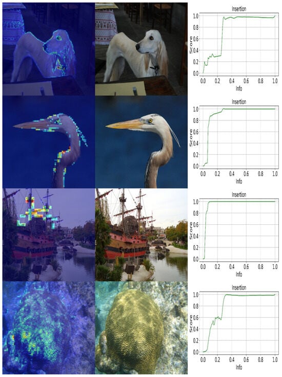
Figure 5. MLFIH examples illustrating samples whose score contributions mainly arise from high-, mid-, low, and mid-and-high-frequency layers. In the Insertion plot, the horizontal axis reflects the wavelet-based synthesis with added frequency components, and the vertical axis shows the cosine similarity score. See Section 4.3.2 and Section 4.1.1 for details.

5. Conclusions

In this work, we introduced the WSG-FEC framework, which explains CNN models from a frequency-domain perspective while combining the efficiency of white-box methods with the high resolution of black-box approaches. By integrating multilevel Haar wavelet decomposition with Grad-CAM, the framework generates hierarchical frequential-spatial saliency maps that overcome the limitations of existing interpretability techniques. Experimental results demonstrate that WSG-FEC achieves a 1.71× improvement in matrix efficiency and completes single-image explanations within 78.26 s on ResNet-50, outperforming conventional methods in both accuracy and computational cost. These findings highlight the potential of frequency-domain representations to provide fine-grained interpretability while maintaining practical feasibility.

The main contributions can be summarized as follows:

• Proposing a gray-box explanation framework that integrates frequency decomposition with weakly supervised learning;
• Providing higher-resolution explanations across multiple frequency levels;
• Achieving a balance between efficiency and accuracy, validated through empirical experiments.

Beyond these contributions, the study demonstrates that frequency-domain interpretability can serve as a general paradigm for enhancing transparency in deep learning models. The ability to capture multi-scale frequency information not only improves the clarity of explanations but also reduces computational overhead, making the approach suitable for real-world applications such as medical image diagnosis, industrial inspection, and video understanding.

Future work will extend this framework to more CNN architectures and application domains and further refine the random optimization strategy to enhance stability and generalization. In addition, exploring hybrid approaches that combine frequency-domain analysis with other interpretability paradigms may open new directions for explainable artificial intelligence.

References

- Bonalumi, L.; Aymerich, E.; Alessi, E.; Cannas, B.; Fanni, A.; Lazzaro, E.; Nowak, S.; Pisano, F.; Sias, G.; Sozzi, C. eXplainable Artificial Intelligence applied to algorithms for disruptions prediction in tokamak devices. Front. Phys. 2024, 12, 1359656. [Google Scholar] [CrossRef]
- Ferreira, D.R.; Martins, T.A.; Rodrigues, P.; Contributors, J.E.T. Explainable deep learning for the analysis of MHD spectrograms in nuclear fusion. Mach. Learn. Sci. Technol. 2021, 3, 015015. [Google Scholar] [CrossRef]
- Zhou, B.; Khosla, A.; Lapedriza, A.; Oliva, A.; Torralba, A. Learning Deep Features for Discriminative Localization. In Proceedings of the IEEE Conference on Computer Vision and Pattern Recognition (CVPR 2016), Las Vegas, NV, USA, 27–30 June 2016; pp. 2921–2929. [Google Scholar]
- Selvaraju, R.R.; Cogswell, M.; Das, A.; Vedantam, R.; Parikh, D.; Batra, D. Grad-CAM: Visual Explanations from Deep Networks via Gradient-Based Localization. In Proceedings of the IEEE International Conference on Computer Vision (ICCV), Venice, Italy, 22–29 October 2017; pp. 618–626. [Google Scholar]
- Chattopadhay, A.; Sarkar, A.; Howlader, P.; Balasubramanian, V. Grad-CAM++: Generalized Gradient-Based Visual Explanations for Deep Convolutional Networks. In Proceedings of the IEEE Winter Conference on Applications of Computer Vision (WACV), Lake Tahoe, NV, USA, 12–15 March 2018; pp. 839–847. [Google Scholar]
- Chen, C.; Li, O.; Tao, D.; Barnett, A.; Rudin, C.; Su, J. This Looks Like That: Deep Learning for Interpretable Image Recognition. In Proceedings of the 33rd Conference on Neural Information Processing Systems (NeurIPS), Vancouver, BC, Canada, 8–14 December 2019. [Google Scholar]
- Stefenon, S.F.; Singh, G.; Yow, K.C.; Cimatti, A. Semi-ProtoPNet Deep Neural Network for the Classification of Defective Power Grid Distribution Structures. Sensors 2022, 22, 4859. [Google Scholar] [CrossRef] [PubMed]
- Singh, G.; Yow, K.C. Object or Background: An Interpretable Deep Learning Model for COVID-19 Detection from CT-Scan Images. Diagnostics 2021, 11, 1732. [Google Scholar] [CrossRef] [PubMed]
- Singh, G. One and One Make Eleven: An Interpretable Neural Network for Image Recognition. Knowl.-Based Syst. 2023, 279, 110926. [Google Scholar] [CrossRef]
- Petsiuk, V.; Das, A.; Saenko, K. RISE: Randomized Input Sampling for Explanation of Black-Box Models. arXiv 2018, arXiv:1806.07421. [Google Scholar] [CrossRef]
- Yan, Y.; Li, X.; Zhan, Y.; Sun, L.; Zhu, J. GSM-HM: Generation of Saliency Maps for Black-Box Object Detection Model Based on Hierarchical Masking. IEEE Access 2022, 10, 98268–98277. [Google Scholar] [CrossRef]
- Kakogeorgiou, I.; Karantzalos, K. Evaluating explainable artificial intelligence methods for multi-label deep learning classification tasks in remote sensing. Int. J. Appl. Earth Obs. Geoinf. 2021, 103, 102520. [Google Scholar] [CrossRef]
- Ribeiro, M.T.; Singh, S.; Guestrin, C. “Why Should I Trust You?”: Explaining the Predictions of Any Classifier. In Proceedings of the 22nd ACM SIGKDD International Conference on Knowledge Discovery and Data Mining, San Francisco, CA, USA, 13–17 August 2016; pp. 1135–1144. [Google Scholar]
- Rabbani, M.; Jones, P. Digital Image Compression Techniques; SPIE Press: Bellingham, WA, USA, 1991. [Google Scholar]
- Xu, Z.Q.J.; Zhang, Y.; Luo, T.; Xiao, Y.; Ma, Z. Frequency Principle: Fourier Analysis Sheds Light on Deep Neural Networks. arXiv 2019, arXiv:1901.06523. [Google Scholar] [CrossRef]
- Huber, M.; Damer, N. Beyond Spatial Explanations: Explainable Face Recognition in the Frequency Domain. In Proceedings of the 2025 IEEE/CVF Winter Conference on Applications of Computer Vision (WACV), Tucson, AZ, USA, 26 February–4 March 2025; pp. 1016–1026. [Google Scholar]
- Huber, M.; Neto, P.C.; Sequeira, A.F.; Damer, N. FX-MAD: Frequency-Domain Explainability and Explainability-Driven Unsupervised Detection of Face Morphing Attacks. In Proceedings of the Winter Conference on Applications of Computer Vision, Tucson, AZ, USA, 28 February–4 March 2025; pp. 766–776. [Google Scholar]
- Chliński, K.; Wawrzyński, P. DCT-Conv: Coding Filters in Convolutional Networks with Discrete Cosine Transform. In Proceedings of the 2020 International Joint Conference on Neural Networks (IJCNN), Glasgow, UK, 19–24 July 2020; pp. 1–6. [Google Scholar]
- Lin, T.Y.; Dollár, P.; Girshick, R.; He, K.; Hariharan, B.; Belongie, S. Feature Pyramid Networks for Object Detection. In Proceedings of the 2017 IEEE Conference on Computer Vision and Pattern Recognition (CVPR), Honolulu, HI, USA, 21–26 July 2017; pp. 936–944. [Google Scholar]
- Xu, Z.; Zhang, Y.; Xiao, Y. Training Behavior of Deep Neural Network in Frequency Domain. In Proceedings of the 26th International Conference on Neural Information Processing (ICONIP 2019), Part I, Sydney, NSW, Australia, 12–15 December 2019; pp. 264–274. [Google Scholar]
- Ding, B.; Zhang, R.; Xu, L.; Liu, G.; Yang, S.; Liu, Y.; Zhang, Q. U 2 D 2 Net: Unsupervised Unified Image Dehazing and Denoising Network for Single Hazy Image Enhancement. IEEE Trans. Multimedia 2023, 26, 202–217. [Google Scholar] [CrossRef]
- Wang, G.; Zhao, W.; Zou, P.; Wang, J.; Yin, H.; Yu, Y. Quantum Image Edge Detection Based on Haar Wavelet Transform. Quantum Inf. Process. 2024, 23, 302. [Google Scholar] [CrossRef]
- ISO/IEC 15444-1:2000; Information Technology—JPEG 2000 Image Coding System: Core Coding System. International Organization for Standardization: Geneva, Switzerland, 2000.
- Alsoufi, M.A.; Siraj, M.M.; Ghaleb, F.A.; Abdulqader, A.H.; Ali, E.; Omar, M. An Anomaly Intrusion Detection Systems in IoT Based on Autoencoder: A Review. In Advances in Intelligent Computing Techniques and Applications. IRICT 2023. Lecture Notes on Data Engineering and Communications Technologies; Springer Nature: Cham, Switzerland, 2023; pp. 224–239. [Google Scholar]
- Qian, J.; Song, Z.; Yao, Y.; Zhu, Z.; Zhang, X. A Review on Autoencoder Based Representation Learning for Fault Detection and Diagnosis in Industrial Processes. Chemom. Intell. Lab. Syst. 2022, 231, 104711. [Google Scholar] [CrossRef]
- Hu, M.; Han, H.; Shan, S.; Chen, X. Weakly Supervised Image Classification through Noise Regularization. In Proceedings of the IEEE/CVF Conference on Computer Vision and Pattern Recognition, Long Beach, CA, USA, 16–20 June 2019; pp. 11517–11525. [Google Scholar]
- Ren, Z.; Wang, S.; Zhang, Y. Weakly supervised machine learning. CAAI Trans. Intell. Technol. 2023, 8, 549–580. [Google Scholar] [CrossRef]
- Durand, T.; Mordan, T.; Thome, N.; Cord, M. WILDCAT: Weakly Supervised Learning of Deep ConvNets for Image Classification, Pointwise Localization and Segmentation. In Proceedings of the IEEE Conference on Computer Vision and Pattern Recognition, Honolulu, HI, USA, 21–26 July 2017; pp. 642–651. [Google Scholar]
- Fong, R.C.; Vedaldi, A. Interpretable Explanations of Black Boxes by Meaningful Perturbation. In Proceedings of the IEEE International Conference on Computer Vision (ICCV), Venice, Italy, 22–29 October 2017; pp. 3429–3437. [Google Scholar]
- Samek, W.; Binder, A.; Montavon, G.; Lapuschkin, S.; Müller, K.R. Evaluating the Visualization of What a Deep Neural Network Has Learned. IEEE Trans. Neural Netw. Learn. Syst. 2016, 28, 2660–2673. [Google Scholar] [CrossRef] [PubMed]
- Valois, P.H.V.; Niinuma, K.; Fukui, K. Occlusion Sensitivity Analysis with Augmentation Subspace Perturbation in Deep Feature Space. In Proceedings of the 2024 IEEE/CVF Winter Conference on Applications of Computer Vision (WACV), Waikoloa, HI, USA, 3–8 January 2024; pp. 4817–4826. [Google Scholar] [CrossRef]
- Yang, M.; Kim, B. Benchmarking Attribution Methods with Relative Feature Importance. arXiv 2019, arXiv:1907.09701. [Google Scholar] [CrossRef]
Disclaimer/Publisher’s Note: The statements, opinions and data contained in all publications are solely those of the individual author(s) and contributor(s) and not of MDPI and/or the editor(s). MDPI and/or the editor(s) disclaim responsibility for any injury to people or property resulting from any ideas, methods, instructions or products referred to in the content. |
© 2025 by the authors. Licensee MDPI, Basel, Switzerland. This article is an open access article distributed under the terms and conditions of the Creative Commons Attribution (CC BY) license.