Parallel Direct Solution of Flexible Multibody Systems Based on Block Gaussian Elimination

Abstract

This paper proposes a parallel direct solution of flexible multibody systems based on block Gaussian elimination. The Craig–Bampton method is utilized to model flexible bodies within the multibody system, resulting in a reduction in the size of the system equations. To address the time integration problem, an implicit stiff scheme is adopted to obtain large time step sizes. When forming the linearized systemic equations, global sparsity in the Jacobian matrix and similar local sparsity in submatrices can be observed. Subsequently, block Gaussian elimination is introduced for the direct solution of these linearized equations. The algorithm is designed to be parallelizable at the algorithm level, with a specific processing order for the submatrices of the constraints. The stability of the method is guaranteed by the positive definite and symmetric properties in the diagonal matrices in the Craig–Bampton method. The parallel efficiency and numerical stability of the method are confirmed through numerical examples in homemade codes parallelized by OpenMP.

1. Introduction

Analysis, design, and optimization of complex flexible multibody systems (FMBS) are often limited by computational efficiency [1]. A potential solution is to develop a modeling method that offers high precision with a reduced number of degrees of freedom (DOFs) and, subsequently, address it using parallel computation.

To reduce the DOFs of flexible parts in multibody systems, the component mode synthesis (CMS) [2,3] methods are widely utilized, where the floating frame of reference (FFR) [2,4] and modal coordinates are introduced to express a flexible body. Among the CMS methods, the fixed-interface Craig–Bampton (CB) method [5,6] is extensively popular. The CB method preserves boundary modes, typically resulting in higher accuracy than the free-interface Craig–Chang method [7,8,9]. Despite this, numerous extensions and improvements have been suggested to enhance the CB method’s precision. Notably, we consider residual flexibility as one of the most successful strategies, which is known as the enhanced Craig–Bampton (ECB) method proposed by Kim [10,11,12,13].

To enhance computational efficiency, large time integration step sizes and high single-step efficiency are typically desired. Implicit methods for solving stiff problems, such as the backward difference formulas (BDFs) [14], can achieve these large step sizes. The resulting nonlinear algebraic equations [2] can then be linearized and solved iteratively [1], for instance, using the Newton iteration as shown by Yang [15].

Parallelization techniques have been adopted in these processes by researchers, aiming for higher efficiency. The assembly process can commonly be significantly accelerated through parallelization, which includes the calculation of general forces, their Jacobian matrices, component modes, and stress recovery. For instance, Park [16] exploited the modular features of the FMBS to achieve active control and real-time applications. Cao [17] computed the residual vector and Jacobian matrix in parallel using OpenMP [18] in a large diesel engine analysis. Negrut [19,20] combined CPU and GPU parallelization to compute contact forces and the contact Jacobian matrix in scenarios with many contacts in multibody systems. Pařík, Kim et al. [21] exploited the substructure independence to obtain a parallel approach for the ECB method. Cros [22] and Murthy [23] applied parallelization in modes generating and component stress recovery for the CB method and some CMS method, respectively. Motivated by the ideal parallelization efficiency in this process, domain decomposition methods have been introduced to divide large FMBS into smaller substructures for better parallelization, as suggested by Li [24], Featherstone [25], Dewes [26], and Cano [27].

After assembly, the linearized systemic equations must be solved. As Wasfy and Noor pointed out in their review [28], parallelizing an implicit and direct solution process is significantly challenging. This is due to the need for decomposing the Jacobian matrix, which involves interdependent operations. Typically, parallel operations can only be performed within a single column, such as within the LU decomposition. Although commercial parallel direct solvers like PARDISO can be used [17], the numerical stability and efficiency for different FMBS models are somehow unclear.

Indeed, the Jacobian matrices generated by the CB method possess unique block sparse structures that have not been fully exploited in current calculation schemes. By leveraging these characteristics and employing the block Gaussian elimination (BGE) method [29,30], we propose an algorithm-level parallel scheme for the direct solution of linearized systemic equations. In the proposed scheme, the Jacobian matrix is eliminated into a small subspace of Lagrange multipliers in a block-wise and fully parallel manner. Once the Lagrange multipliers are resolved, the reverse substitution can also be executed in full parallel. Moreover, by considering the matrix bandwidth, the block matrix sparsity can be retained with specific block order arrangement. The numerical stability is guaranteed by the BGE stability criterion.

This paper is arranged as follows. Section 2 details the formulation of multibody systems, with flexible components modeled by the Craig–Bampton method. Procedure details of algebraic-differential governing equations, implicit integration scheme, equation linearization and assembly, DOFs reduction by the Craig–Bampton method, rigid modes removing and modes orthogonalization, and flexible body formulation under floating frame of reference are illustrated sequentially. In Section 3, we propose a parallel direct solution scheme based on block Gaussian elimination. Coordinate reordering is applied to generate a small bandwidth within the Jacobian matrix and its submatrices, and the feasibility of the sub-block Jacobian matrix is studied. The block and sparse features of the presented Jacobian matrix are deeply investigated, and subsequently, we introduce the block Gaussian elimination method to solve the linear equations at an algorithmic level of parallelism. Section 4 verifies the effectiveness and efficiency of the algorithm through numerical examples, which include the vibration of an aeroengine stator system and the rotation of a crank-slider mechanism.

2. Flexible Multibody Formulation with the Craig–Bampton Method

This section details the flexible multibody formulation with the Craig–Bampton method. For system governing equations, the Lagrange equations of the first kind are adopted for convenience of code implementation. The resulting algebraic-differential equations are time-discretized using the implicit integration method, specifically backward difference formulas, to accommodate large time step sizes. The flexible body formulation using the Craig–Bampton method is then detailed, encompassing the DOFs reduction process and the generation of mass and stiffness matrices. In a subsequent section, a feature study of these matrices is the prerequisite for the presented algorithm-level parallel.

2.1. Time Integration Procedures of Flexible Multibody Systems

2.1.1. System Governing Equations

The Lagrange equations of the first kind are utilized to express the governing equations of the flexible multibody system [2] as

$$\left\{\begin{array}{l}{\displaystyle \frac{\mathrm{d}}{\mathrm{d}t}}\left({\displaystyle \frac{\partial L(\xi ,\dot{\xi })}{\partial \xi }}\right)-{\displaystyle \frac{\partial L(\xi ,\dot{\xi })}{\partial \xi }}+{\left({\displaystyle \frac{\partial c}{\partial \xi }}\right)}^{\mathrm{T}}\lambda =\tau ,\\ c\left(\xi \right)=0,\end{array}\right.$$

(1)

wherein $\xi$ is the general displacement of the bodies, $L=T-V$ denotes the Lagrange function with the system’s kinetic energy $T$ and potential energy $V$, $\tau$ is the general force vector of the external loads, $c$ is a set of complete constraint equations that are solely dependent on the general displacement $\xi$, and $\lambda$ corresponds to the Lagrangian multipliers of the constrains.

The constraints between bodies are explicitly expressed by the algebraic equations $c\left(\xi \right)=0$ in Equation (1). This facilitates convenient computer coding. However, the variable $\lambda$ has the same magnitude as the constraint forces and often introduces numerical problems due to its large difference in magnitude compared to the general displacement variable $\xi$. This issue can be effectively resolved by multiplying the constraint equations $c\left(\xi \right)=0$ by a scale factor $a$ to balance the magnitudes between $\xi$ and $\lambda$, as follows:

$$\left\{\begin{array}{l}{\displaystyle \frac{\mathrm{d}}{\mathrm{d}t}}\left({\displaystyle \frac{\partial L(\xi ,\dot{\xi })}{\partial \xi }}\right)-{\displaystyle \frac{\partial L(\xi ,\dot{\xi })}{\partial \xi }}+{\left(a\cdot {\displaystyle \frac{\partial c}{\partial \xi }}\right)}^{\mathrm{T}}\lambda =\tau ,\\ a\cdot c\left(\xi \right)=0.\end{array}\right.$$

(2)

A method for calculating the scale factor $a$ has been detailed in the authors’ previous work [31], and readers are encouraged to consult it for further information. Since Equation (2) does not differ fundamentally from Equation (1), we still use Equation (1) instead of Equation (2) by taking $c$ as $a\cdot c$ in Equation (1).

In Equation (1), the Lagrange function relating terms are actually the general inertial forces $F_{\mathrm{iner}}$ and general elastic forces $F_{\mathrm{elas}}$, and they are the internal forces within the bodies. By separating them from the external forces $\tau$ and constraint forces $c_{\xi }^{\mathrm{T}}\lambda$, the system governing equation can be rewritten as

$$\left\{\begin{array}{l}{F}_{\mathrm{iner}}(\xi ,\dot{\xi },\ddot{\xi })+F_{\mathrm{elas}}(\xi )=\tau (\xi ,\dot{\xi })-c_{\xi }^{\mathrm{T}}(\xi )\lambda \hspace{0.33em},\\ c(\xi )=0\hspace{0.33em},\end{array}\right.$$

(3)

wherein $c_{\xi }^{\mathrm{T}}$ is the abbreviation of ${(\partial c/\partial \xi )}^{\mathrm{T}}$.

2.1.2. Time Integration Scheme

To solve the algebraic-differential Equation (3), we need to apply a time integration to convert the general velocity $\dot{\xi }$ and acceleration $\ddot{\xi }$ into displacement $\xi$ at the time integration steps. Since multibody problems are typically stiff, meaning that the system responses contain both low and high frequencies simultaneously, the stiff integrator—backward difference formulas (BDFs) is utilized in this paper.

For simplicity, we use a constant step size $h$ and the first-order BDFs to demonstrate the integration process. To avoid confusion, we also employ a right superscript within parentheses ${\square }^{(n)}$ to denote variable values at the discrete time $t=nh$, such as ${\xi }^{(n)}\triangleq {\left.\xi \right|}_{t=nh}$ and ${\lambda }^{(n)}\triangleq {\left.\lambda \right|}_{t=nh}$. Assuming the previous $n-1$ time steps are known and the $n^{\mathrm{th}}$ time step needs to be computed, the general velocity and acceleration can be expressed in terms of displacement as

$$\left\{\begin{array}{l}{\dot{\xi }}^{(n)}={\displaystyle \frac{{\xi }^{(n)}-{\xi }^{(n-1)}}{h}}\triangleq f_{\mathrm{v}}({\xi }^{(n)}),\\ {\ddot{\xi }}^{(n)}={\displaystyle \frac{{\dot{\xi }}^{(n)}-{\dot{\xi }}^{(n-1)}}{h}}={\displaystyle \frac{{\xi }^{(n)}-2{\xi }^{(n-1)}+{\xi }^{(n-2)}}{h^2}}\triangleq f_{\mathrm{a}}({\xi }^{(n)}),\end{array}\right.$$

(4)

wherein $f_{\mathrm{v}}$ represents the velocity’s algebraic function and $f_{\mathrm{a}}$ represents the acceleration’s algebraic function.

Readers may notice that Formula (4) is not applicable when $n=1$, where ${\xi }^{(-1)}$ is requested in forming ${\ddot{\xi }}^{(1)}$. A possible solution is to estimate ${\xi }^{(-1)}$ using the Taylor series as

$${\xi }^{(-1)}={\xi }^{(0)}-{\dot{\xi }}^{(0)}h+{\ddot{\xi }}^{(0)}{\displaystyle \frac{h^2}{2}}+o(h^2),$$

(5)

wherein ${\xi }^{(0)}$ and ${\dot{\xi }}^{(0)}$ are given by the initial conditions and ${\ddot{\xi }}^{(0)}$ can be calculated by solving the system Equation (3) at time $t=0$.

By substituting Equation (4) into Equation (3), nonlinear algebraic equations at the time step $t=nh$ with unknown variables ${\xi }^{(n)}$ and ${\lambda }^{(n)}$ are obtained as

$$\left\{\begin{array}{l}{F}_{\mathrm{iner}}\left({\xi }^{(n)},f_{\mathrm{v}}({\xi }^{(n)}),f_{\mathrm{a}}({\xi }^{(n)})\right)+F_{\mathrm{elas}}\left({\xi }^{(n)}\right)=\tau \left({\xi }^{(n)},f_{\mathrm{v}}({\xi }_{nh})\right)-c_{\xi }^{\mathrm{T}}({\xi }^{(n)}){\lambda }^{(n)},\\ c({\xi }^{(n)})=0,\end{array}\right.$$

(6)

wherein the nonlinearity may arise from the expression of $F_{\mathrm{iner}}$, $F_{\mathrm{elas}}$, $\tau$, and $c$.

2.1.3. Equation Linearization and Assembly

The nonlinear algebraic Equation (6) can then be linearized and solved iteratively, for instance, using the Newton iteration, as shown in our previous work [15].

To start the Newton iteration, an initial guess close enough is needed for ${\xi }^{(n)}$. With the first-order constant step BDFs, the initial guess of the differential variable ${\xi }^{(n)}$ is simply given by the same order extrapolation formula as

$${\xi }^{(n,0)}=2{\xi }^{(n-1)}-{\xi }^{(n-2)},$$

(7)

wherein the two numbers in the right superscript, enclosed by parenthesis ${\square }^{(n,j)}$, represent the results of the $j^{\mathrm{th}}$ iteration for the $n^{\mathrm{th}}$ time step. Consequently, ${\xi }^{(n,0)}$ represents the initial value in the iteration for the $n^{\mathrm{th}}$ time step.

The Lagrange multipliers are not differentiable with respect to time, and the initial guess is set to zero as

$${\lambda }^{(n,0)}=0.$$

(8)

We rewrite the nonlinear Equation (6) on one side to obtain their residual form:

$$\left\{\begin{array}{l}b({\xi }^{(n)})\triangleq F_{\mathrm{iner}}\left({\xi }^{(n)},f_{\mathrm{v}}({\xi }^{(n)}),f_{\mathrm{a}}({\xi }^{(n)})\right)+F_{\mathrm{elas}}\left({\xi }^{(n)}\right)-\tau \left({\xi }_{nh},f_{\mathrm{v}}({\xi }_{nh})\right)+c_{\xi }^{\mathrm{T}}({\xi }^{(n)}){\lambda }^{(n)}=0\hspace{0.33em},\\ c({\xi }^{(n)})=0\hspace{0.33em},\end{array}\right.$$

(9)

and the Newton iteration is given by

$$\left[\begin{array}{cc}{\displaystyle \frac{\partial b}{\partial {\xi }^{(n)}}}& {\left({\displaystyle \frac{\partial c}{\partial {\xi }^{(n)}}}\right)}^{\mathrm{T}}\\ {\displaystyle \frac{\partial c}{\partial {\xi }^{(n)}}}& 0\end{array}\right]\left[\begin{array}{c}\Delta {\xi }^{(n,j)}\\ \Delta {\lambda }^{(n,j)}\end{array}\right]=-\left[\begin{array}{c}b({\xi }^{(n,j)})\\ c({\xi }^{(n,j)})\end{array}\right],$$

(10)

wherein

$${\displaystyle \frac{\partial b}{\partial {\xi }^{(n)}}}={\displaystyle \frac{\partial F_{\mathrm{iner}}}{\partial \xi }}+{\displaystyle \frac{\partial F_{\mathrm{iner}}}{\partial \dot{\xi }}}{\displaystyle \frac{\partial f_{\mathrm{v}}}{\partial {\xi }^{(n)}}}+{\displaystyle \frac{\partial F_{\mathrm{iner}}}{\partial \ddot{\xi }}}{\displaystyle \frac{\partial f_{\mathrm{a}}}{\partial {\xi }^{(n)}}}+{\displaystyle \frac{\partial F_{\mathrm{elas}}}{\partial \xi }}-{\displaystyle \frac{\partial \tau }{\partial \xi }}-{\displaystyle \frac{\partial \tau }{\partial \dot{\xi }}}{\displaystyle \frac{\partial f_{\mathrm{v}}}{\partial {\xi }^{(n)}}}+{\displaystyle \frac{\partial \left(c_{\xi }^{\mathrm{T}}{\lambda }^{(n)}\right)}{\partial \xi }}.$$

(11)

Typically, the second-order differential term ${\displaystyle \frac{\partial \left(c_{\xi }^{\mathrm{T}}{\lambda }^{(n)}\right)}{\partial \xi }}$ is omitted in Formula (11) to ensure the stability of the Newton iteration because of the quick variation in the variable ${\lambda }^{(n)}$. Utilizing the time discrete Formula (4), we have

$${\displaystyle \frac{\partial f_{\mathrm{v}}}{\partial {\xi }^{(n)}}}={\displaystyle \frac{1}{h}},\hspace{0.33em}{\displaystyle \frac{\partial f_{\mathrm{a}}}{\partial {\xi }^{(n)}}}={\displaystyle \frac{1}{h^2}},$$

(12)

and denote the linearized general mass, damping, and stiffness matrices of the bodies as

$$M\triangleq {\displaystyle \frac{\partial F_{\mathrm{iner}}}{\partial \ddot{\xi }}},C\triangleq {\displaystyle \frac{\partial F_{\mathrm{iner}}}{\partial \dot{\xi }}},K\triangleq {\displaystyle \frac{\partial F_{\mathrm{elas}}}{\partial \xi }}+{\displaystyle \frac{\partial F_{\mathrm{iner}}}{\partial \xi }},$$

(13)

The Newton iteration (10) for the nonlinear Equation (9) is rewritten as

$${\left[\begin{array}{cc}{\displaystyle \frac{M}{h^2}}+{\displaystyle \frac{C}{h}}+K-\left({\displaystyle \frac{\partial \tau }{\partial \xi }}+{\displaystyle \frac{1}{h}}\cdot {\displaystyle \frac{\partial \tau }{\partial \dot{\xi }}}\right)& \hfill {\displaystyle \frac{\partial c^{\mathrm{T}}}{\partial \xi }}\\ {\displaystyle \frac{\partial c}{\partial \xi }}& \hfill 0\end{array}\right]}^{(n,j)}\left[\begin{array}{c}\Delta {\xi }^{(n,j)}\\ \Delta {\lambda }^{(n,j)}\end{array}\right]=-{\left[\begin{array}{c}b\\ c\end{array}\right]}^{(n,j)},$$

(14)

wherein the Jacobian matrix and the right-hand terms are calculated at variables ${\xi }^{(n,j)}$ and ${\lambda }^{(n,j)}$. The terms related to the external forces $\tau$ are enclosed with parenthesis.

After $\Delta {\xi }^{(n,j)}$ and $\Delta {\lambda }^{(n,j)}$ are solved by a linear solver, the iteration proceeds from $j$ to $j+1$ as

$${\xi }^{(n,j+1)}={\xi }^{(n,j)}+\Delta {\xi }^{(n,j)},$$

(15)

until the following convergence errors are satisfied:

$$\left|\right|\Delta {\xi }^{(n,j)}\left|\right|\le e_{\xi },\left|\right|\Delta {\lambda }^{(n,j)}\left|\right|\le e_{\lambda },\left|\right|b^{(n,j)}\left|\right|\le e_b,\left|\right|c^{(n,j)}\left|\right|\le e_c,$$

(16)

wherein $\left|\right|\square \left|\right|$ represents an arbitrary given norm and $e_{\xi }$, $e_{\lambda }$, $e_b$, and $e_c$ are the corresponding error thresholds for displacement variables, constraint forces, body equation residuals, and constraint equation residuals, respectively.

Let the system consist of $m$ bodies and $k$ constraints. Then, the system vector of body DOFs is $\xi =\left[{\xi }_1;\cdots ;{\xi }_m\right]$, and the system vector of constraint multipliers is $\lambda =\left[{\lambda }_1;\cdots ;{\lambda }_k\right]$. To assemble Equation (14), we need to calculate

$$K=\mathrm{diag}(K_1,\cdots ,K_m),C=\mathrm{diag}(C_1,\cdots ,C_m),M=\mathrm{diag}(M_1,\cdots ,M_m),\tau =\left[{\tau }_1;\cdots ;{\tau }_m\right],$$

(17)

and

$$c=\left[c_1;\cdots ;c_k\right],\hspace{0.33em}{\displaystyle \frac{\partial c}{\partial \xi }}=\left[{\displaystyle \frac{\partial c_1}{\partial \xi }};\cdots ;{\displaystyle \frac{\partial c_k}{\partial \xi }}\right]$$

(18)

wherein the subscript indicates which body or constraint the variable or matrix belongs to, while the semicolon “;” separates the components of a “column” vector. Additionally, $\mathrm{diag}(\cdots )$ signifies that the matrix is block-diagonally composed of submatrices.

Since the flexible bodies are modeled using the Craig–Bampton method in this paper, we will elaborate on how the general mass matrix $M_i$ and stiffness matrix $K_i$ $(i=1,\cdots ,m)$ are computed in the subsection. The damping matrix $C_i$ may be omitted in an undamped case or be considered as a linear combination of $M_i$ and $K_i$ under a Rayleigh damping hypothesis.

2.2. Flexible Body Formulation with the Craig–Bampton Method

2.2.1. DOFs Reduction by the Craig–Bampton Method

To reduce the degrees of freedom (DOFs) of flexible parts in multibody systems, the component mode synthesis (CMS) [2,3] methods are widely utilized. In all CMS methods, the first step is to calculate the preserved modes of the flexible parts under specified boundary conditions. For the Craig–Bampton (CB) method [5,6], all interfaces for joint connections and force applications are fixed when calculating the inner flexible modes. Hence, the CB method is also referred to as a fixed-interface method. Only a few inner modes are preserved to reduce the DOFs of a flexible part. To express the connections and forces acting on the flexible body, static response modes for each boundary DOF are also calculated and preserved, which are known as the boundary modes. The boundary modes are indeed static equilibrium configurations of the flexible body when a single boundary DOF moves a unit displacement in its own direction.

Before performing the modes calculation of the flexible body $i$, we first separate the inner DOFs $u_i^{\Lambda }$ and boundary DOFs $u_i^{\Gamma }$ within the finite element (FE) formulation. Superscripts ${\square }^{\Lambda }$ and ${\square }^{\Gamma }$ denote the inner DOFs and boundary DOFs, respectively. Set $u_i=[u_i^{\Gamma };u_i^{\Lambda }]$ and rearrange the FE equations to obtain

$$\underset{{\overline{K}}_i}{\underbrace{\left[\begin{array}{cc}{\overline{K}}_i^{\Gamma \Gamma }& {\overline{K}}_i^{\Gamma \Lambda }\\ {\overline{K}}_i^{\Lambda \Gamma }& {\overline{K}}_i^{\Lambda \Lambda }\end{array}\right]}}\left[\begin{array}{c}{u}_i^{\Gamma }\\ u_i^{\Lambda }\end{array}\right]+\underset{{\overline{M}}_i}{\underbrace{\left[\begin{array}{cc}{\overline{M}}_i^{\Gamma \Gamma }& {\overline{M}}_i^{\Gamma \Lambda }\\ {\overline{M}}_i^{\Lambda \Gamma }& {\overline{M}}_i^{\Lambda \Lambda }\end{array}\right]}}\left[\begin{array}{c}{\ddot{u}}_i^{\Gamma }\\ {\ddot{u}}_i^{\Lambda }\end{array}\right]=\left[\begin{array}{c}{\overline{f}}_i\\ 0\end{array}\right],$$

(19)

wherein ${\overline{K}}_i$ represents the stiffness matrix and ${\overline{M}}_i$ represents the mass matrix. ${\overline{f}}_i$ denotes the external forces applied to the boundary DOFs.

To obtain the inner modes, we fix the boundary DOFs and set $u_i^{\Gamma }={\ddot{u}}_i^{\Gamma }={\overline{f}}_i=0$ in Equation (19) to obtain

$${\overline{K}}_i^{\Lambda \Lambda }{u}_i^{\Lambda }+{\overline{M}}_i^{\Lambda \Lambda }{\ddot{u}}_i^{\Lambda }=0.$$

(20)

Then, the vibration Equation (20) is solved, and the first $N_i$ low-frequency modes ${\overline{\phi }}_{i,j}^{\Lambda } (j=1,\cdots ,N_i)$ are preserved for coordinates $u_i^{\Lambda }$. These modes are extended to the full DOFs $u_i$, and we have the vibration modes matrix as follows:

$${\overline{\Phi }}_i^{\mathrm{vibr}}=\left[\begin{array}{ccc}0& \cdots & 0\\ {\overline{\phi }}_{i,1}^{\Lambda }& \cdots & {\overline{\phi }}_{i,N_i}^{\Lambda }\end{array}\right].$$

(21)

Assuming the number of boundary DOFs for flexible body $i$ is $M_i$, a total of $M_i$ boundary modes need to be calculated. To obtain the $j^{\mathrm{th}}$ boundary mode, we ignore the inertial force term and the external forces and set $u_i^{\Gamma }=[0;\cdots ;0;1;0;\cdots ;0]$ with the only 1 at the $j^{\mathrm{th}}$ coordinate in Equation (19) to obtain

$$\left[\begin{array}{c}{\overline{k}}_{i,j}^{\Gamma \Gamma }\\ {\overline{k}}_{i,j}^{\Lambda \Gamma }\end{array}\right]+\left[\begin{array}{c}{\overline{K}}_i^{\Gamma \Lambda }\\ {\overline{K}}_i^{\Lambda \Lambda }\end{array}\right]u_i^{\Lambda }=\left[\begin{array}{c}0\\ 0\end{array}\right],j=1,\cdots ,M_i.$$

(22)

wherein ${\overline{k}}_{i,j}^{\Gamma \Gamma }$ and ${\overline{k}}_{i,j}^{\Lambda \Gamma }$ are the $j^{\mathrm{th}}$ column of ${\overline{K}}_i^{\Gamma \Gamma }$ and ${\overline{K}}_i^{\Lambda \Gamma }$, respectively. By solving the static equilibrium Equation (22), we obtain the static equilibrium ${\overline{\psi }}_{i,j}^{\Lambda } (j=1,\cdots ,M_i)$ for the coordinates $u_i^{\Lambda }$. Extending these results to the full DOFs $u_i$ in conjunction with the hypothesis $u_i^{\Gamma }=[0;\cdots ;0;1;0;\cdots ;0]$, we arrive at the boundary modes matrix as follows:

$${\overline{\Phi }}_i^{\mathrm{boun}}=\left[\begin{array}{c}I\\ \begin{array}{ccc}{\overline{\psi }}_{i,1}^{\Lambda }& \cdots & {\overline{\psi }}_{i,M_i}^{\Lambda }\end{array}\end{array}\right].$$

(23)

With the inner vibration modes matrix ${\overline{\Phi }}_i^{\mathrm{vibr}}$ and the boundary modes matrix ${\overline{\Phi }}_i^{\mathrm{boun}}$, a total of $M_i+N_i$ modes are preserved for reduction in DOFs in the flexible body $i$. The preserved modes matrix is

$${\overline{\Phi }}_i=\left[\begin{array}{cc}{\overline{\Phi }}_i^{\mathrm{vibr}}& {\overline{\Phi }}_i^{\mathrm{boun}}\end{array}\right].$$

(24)

2.2.2. Rigid Modes Removing and Modes Orthogonalization

However, there are two defects in the modes set (24). Firstly, rigid modes with zero frequency exist in the subspace generated by the boundary modes ${\Phi }_i^{\mathrm{boun}}$; and secondly, the columns in ${\Phi }_i^{\mathrm{boun}}$ are not orthogonal to those in ${\Phi }_i^{\mathrm{vibr}}$. Rigid modes are redundant because they have been accounted for by the floating frame of reference (FFR) coordinates, while modal orthogonality is essential for producing diagonal modal matrices of stiffness and mass.

To address the two issues, reorthogonalization can be applied. First, we project Equation (19) onto the subspace of ${\overline{\Phi }}_i$ by letting ${\overline{f}}_i=0$, substituting $u_i={\overline{\Phi }}_i{\overline{q}}_i$, and multiplying ${\overline{\Phi }}_i^{\mathrm{T}}$ on the left side, resulting in

$$\left({\overline{\Phi }}_i^{\mathrm{T}}{\overline{K}}_i{\overline{\Phi }}_i\right){\overline{q}}_i+\left({\overline{\Phi }}_i^{\mathrm{T}}\overline{M}{\overline{\Phi }}_i\right){\ddot{\overline{q}}}_i=0,$$

(25)

wherein ${\overline{q}}_i$ represents the redundant modal coordinates corresponding to modes ${\overline{\Phi }}_i$. Secondly, we conduct a mode analysis on the projected vibration Equation (25) to derive the orthogonal modes [32]. By discarding zero-frequency modes and arranging the frequencies in descending order, the reorthogonalized non-zero-frequency modal matrix ${\overline{\overline{\Phi }}}_i$ can fulfill the following unit orthogonal condition corresponding to the mass matrix:

$${\overline{\overline{\Phi }}}_i^{\mathrm{T}}{\overline{\Phi }}_i^{\mathrm{T}}{\overline{M}}_i{\overline{\Phi }}_i{\overline{\overline{\Phi }}}_i=E_{n_i},{\overline{\overline{\Phi }}}_i^{\mathrm{T}}{\overline{\Phi }}_i^{\mathrm{T}}{\overline{K}}_i{\overline{\Phi }}_i{\overline{\overline{\Phi }}}_i={\Omega }_i^2,$$

(26)

wherein $E_{n_i}$ represents the unit matrix with dimension $n_i=M_i+N_i-6$ and ${\Omega }_i^2=\mathrm{diag}({\omega }_{i,1}^2,\cdots ,{\omega }_{i,n_i}^2)$ is the diagonal matrix with non-zero modal circle frequencies ${\omega }_{i,1}\ge \cdots \ge {\omega }_{i,n_i}>0$ in descending order.

Then, the orthogonal non-zero-frequency elastic modes matrix of the CB method is

$${\Phi }_i={\overline{\Phi }}_i{\overline{\overline{\Phi }}}_i\triangleq \left[\begin{array}{ccc}{\phi }_{i,1}& \cdots & {\phi }_{i,n_i}\end{array}\right].$$

(27)

The FE displacement is then expressed by the modal coordinates $q_i=[q_{i,1};q_{i,2},\cdots ;q_{i,n_i}]$ as

$$u_i={\Phi }_i{q}_i,$$

(28)

and the elastic vibration equations of flexible body $i$ are diagonal:

$${\Omega }_i^2{q}_i+{\ddot{q}}_i=f_i,$$

(29)

wherein $f_i={\Phi }_i^{\mathrm{T}}{\overline{f}}_i$ is the modal force of the external forces acting on the flexible body $i$.

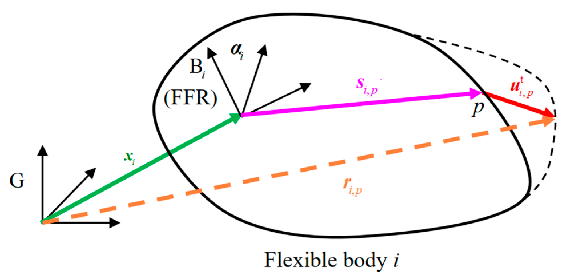
2.2.3. Flexible Body Formulation Under Floating Frame of Reference

The orthogonal modes ${\Phi }_i$ and the elastic coordinates $q_i$ describe the elastic vibration of the flexible body $i$, while the floating frame of reference (FFR) [2] can describe its overall spatial displacement and finite rotation.

Figure 1 shows the coordinates of flexible body $i$ in the FFR. $\mathrm{G}$ represents the global coordinate frame, and ${\mathrm{B}}_i$ presents the body coordinate frame (also the FFR) of flexible body $i$. $x_i=[x_i;y_i;z_i]$ presents the position (column) vector from $\mathrm{G}$ to ${\mathrm{B}}_i$ expressed in $\mathrm{G}$, and ${\alpha }_i=[{\alpha }_i;{\beta }_i;{\gamma }_i]$ presents the rotation parameters from $\mathrm{G}$ to ${\mathrm{B}}_i$. $s_{i,p}$ represents the original position of a node $p$ in ${\mathrm{B}}_i$, and $u_{i,p}^{\mathrm{t}}$ is the translational displacement of node $p$ due to flexible deformation.

Figure 1. Coordinates of flexible body $i$ in the floating frame of reference.

Let $A_i=A_i({\alpha }_i)$ be the transformation matrix from frame ${\mathrm{B}}_i$ to $\mathrm{G}$, and let ${\Phi }_{i,p}$ be the components of the model matrix ${\Phi }_i$ at node $p$. After rigid motion and flexible deformation, the global position of node $p$ on flexible body $i$ is then expressed as

$$r_{i,p}=x_i+A_i(s_{i,p}+u_{i,p}^{\mathrm{t}}),$$

(30)

wherein translational displacement $u_{i,p}^{\mathrm{t}}$ can be expressed with the modal coordinates $q_i$ and ${\Phi }_{i,p}^{\mathrm{t}}$ (i.e., the translational component of the modal matrix ${\Phi }_{i,p}$) as

$$u_{i,p}^{\mathrm{t}}={\Phi }_{i,p}^{\mathrm{t}}{q}_i.$$

(31)

By differentiating the displacement (30) with respect to time, the global velocity of node $p$ is obtained as

$$v_{i,p}={\dot{x}}_i+A_i({\dot{s}}_{i,p}+{\dot{u}}_{i,p})+{\dot{A}}_i(s_{i,p}+u_{i,p}).$$

(32)

wherein $\dot{\square }$ is the time derivative of $\square$, i.e., $\dot{\square }=(\mathrm{d}\square )/(\mathrm{d}t)$. Since $s_{i,p}$ and ${\Phi }_{i,p}^{\mathrm{t}}$ are constant, we have

$${\dot{s}}_{i,p}=0,\hspace{0.33em}\hspace{0.33em}{\dot{u}}_{i,p}=\mathrm{d}({\Phi }_{i,p}^{\mathrm{t}}{q}_i)/\mathrm{d}t={\Phi }_{i,p}^{\mathrm{t}}{\dot{q}}_i.$$

(33)

Since the component ${\dot{A}}_i(s_{i,p}+u_{i,p})$ is caused by rotation of FFR ${\mathrm{B}}_i$ with the vector $(s_{i,p}+u_{i,p})$ on it, we utilize the finite rotation theory to obtain

$${\dot{A}}_i(s_{i,p}+u_{i,p})=A_i\left[{\omega }_i\times (s_{i,p}+u_{i,p})\right]=A_i\left[-(s_{i,p}+u_{i,p})\times {\omega }_i\right]=-A_i({\tilde{s}}_{i,p}+{\tilde{u}}_{i,p}){\omega }_i,$$

(34)

wherein ${\omega }_i$ represents the local (expressed in ${\mathrm{B}}_i$) angular velocity of the frame ${\mathrm{B}}_i$, “$\times$” represents the vector cross-product operation, and ${\tilde{s}}_{i,p}$ projects the vector cross product into a matrix formulation with $s_{i,p}\times {\omega }_i={\tilde{s}}_{i,p}{\omega }_i$ by defining

$${\tilde{s}}_{i,p}=\widetilde{\left[\begin{array}{c}{s}_{i,p,1}\\ s_{i,p,2}\\ s_{i,p,3}\end{array}\right]}\triangleq \left[\begin{array}{ccc}0& -s_{i,p,3}& s_{i,p,2}\\ s_{i,p,3}& 0& -s_{i,p,1}\\ -s_{i,p,2}& s_{i,p,1}& 0\end{array}\right],{\tilde{u}}_{i,p}=\widetilde{\left[\begin{array}{c}{u}_{i,p,1}\\ u_{i,p,2}\\ u_{i,p,3}\end{array}\right]}\triangleq \left[\begin{array}{ccc}0& -u_{i,p,3}& u_{i,p,2}\\ u_{i,p,3}& 0& -u_{i,p,1}\\ -u_{i,p,2}& u_{i,p,1}& 0\end{array}\right].$$

(35)

As shown in reference [2], we can always find a coefficient matrix $D_i=D_i({\alpha }_i)$ for given attitude parameters ${\alpha }_i$ to obtain

$${\omega }_i=D_i{\dot{\alpha }}_i,$$

(36)

Then, the global velocity of node $p$ can be written as

$$v_{i,p}={\dot{x}}_i+A_i{\Phi }_{i,p}^{\mathrm{t}}{\dot{q}}_i-A_i({\tilde{s}}_{i,p}+{\tilde{u}}_{i,p})D_i{\dot{\alpha }}_i.$$

(37)

Different from other references, we place the elastic coordinates $q_i=[q_{i,1};\cdots ;q_{i,n_i}]$ at the forefront to assemble the generalized coordinates of the flexible body $i$ as

$${\xi }_i=\left[q_i;x_i;{\alpha }_i\right]=\left[q_{i,1};\cdots ;q_{i,n_i};x_i;y_i;z_i;{\alpha }_i;{\beta }_i;{\gamma }_i\right].$$

(38)

The mass and stiffness matrices of a flexible body can be obtained by calculating the overall kinetic and potential energies. In the finite element method, the kinetic energy is attributed to the nodes, and with the node mass $m_{i,p}$ and the moment of inertia $H_{i,p}$ lumped at node $p$, we have

$$T_i\approx {\displaystyle \frac{1}{2}}{\displaystyle \sum _p\left(m_{i,p}{v}_{i,p}^{\mathrm{T}}{v}_{i,p}+{\omega }_{i,p}^{\mathrm{T}}{H}_{i,p}{\omega }_{i,p}\right)}.$$

(39)

By substituting Equation (37) into Formula (39) and ignoring high-order quantities of the modal correlation parts, we have

$$\begin{array}{l}{m}_{i,p}{v}_{i,p}^{\mathrm{T}}{v}_{i,p}+{\omega }_{i,p}^{\mathrm{T}}{H}_{i,p}{\omega }_{i,p}=\\ {\dot{\xi }}_i^{\mathrm{T}}\left[\begin{array}{ccc}{m}_{i,p}{({\Phi }_{i,p}^{\mathrm{t}})}^{\mathrm{T}}{\Phi }_{i,p}^{\mathrm{t}}+{({\Phi }_{i,p}^{\mathrm{r}})}^{\mathrm{T}}{H}_{i,p}{\Phi }_{i,p}^{\mathrm{r}}& m_{i,p}{({\Phi }_{i,p}^{\mathrm{t}})}^{\mathrm{T}}{A}_i^{\mathrm{T}}& m_{i,p}{({\Phi }_{i,p}^{\mathrm{t}})}^{\mathrm{T}}({\tilde{s}}_{i,p}^{\mathrm{T}}+{\tilde{u}}_{i,p}^{\mathrm{T}})D_i+{({\Phi }_{i,p}^{\mathrm{r}})}^{\mathrm{T}}{H}_{i,p}{D}_i\\ \mathrm{sym}& m_{i,p}{E}_3& -A_i{m}_{i,p}({\tilde{s}}_{i,p}+{\tilde{u}}_{i,p})D_i\\ \mathrm{sym}& \mathrm{sym}& D_i^{\mathrm{T}}\left[m_{i,p}({\tilde{s}}_{i,p}^{\mathrm{T}}+{\tilde{u}}_{i,p}^{\mathrm{T}})({\tilde{s}}_{i,p}+{\tilde{u}}_{i,p})+H_{i,p}\right]D_i\end{array}\right]{\dot{\xi }}_i\end{array}$$

(40)

wherein, for flexible body $i$, $m_{i,p}$ is the lumped mass at node $p$, $H_{i,p}$ is the symmetric lumped inertia matrix at node $p$, ${\Phi }_{i,p}^{\mathrm{t}}$ is the translational components of the modes ${\Phi }_i$ at node $p$, while ${\Phi }_{i,p}^{\mathrm{r}}$ is the rotational components of the modes ${\Phi }_i$ at node $p$, ${\phi }_{i,p,j}^{\mathrm{t}}$ is the $j^{\mathrm{th}}$ column of ${\Phi }_{i,p}^{\mathrm{t}}$, the wave upon represents the cross-production-to-matrix operator as the same as in Formula (35), and $s_{i,p}$ is the original position of node $p$ in the FFR as shown in Figure 1.

The unit orthogonal condition corresponding to the mass matrix as defined in Equation (26) gives

$$m_{i,p}{({\Phi }_{i,p}^{\mathrm{t}})}^{\mathrm{T}}{\Phi }_{i,p}^{\mathrm{t}}+{({\Phi }_{i,p}^{\mathrm{r}})}^{\mathrm{T}}{H}_{i,p}{\Phi }_{i,p}^{\mathrm{r}}=E_{n_i},$$

(41)

Then, we substitute Formula (40) into the kinetic energy (39) to obtain the generalized mass matrix of the flexible body under the coordinates ${\xi }_i$ as

$$M_i=\left[\begin{array}{ccc}{M}_i^{\mathrm{ff}}& M_i^{\mathrm{ft}}& M_i^{\mathrm{fr}}\\ M_i^{\mathrm{tf}}& M_i^{\mathrm{tt}}& M_i^{\mathrm{tr}}\\ M_i^{\mathrm{rf}}& M_i^{\mathrm{rt}}& M_i^{\mathrm{rr}}\end{array}\right]=\left[\begin{array}{ccc}{E}_{n_i}\hfill & I_{i,3}^{\mathrm{T}}{A}_i^{\mathrm{T}}& I_{i,4}^{\mathrm{T}}{D}_i\\ \mathrm{sym}\hfill & I_{i,1}{E}_3& -A_i({\widetilde{I_{i,2}+I_{i,3}q}}_i)D_i\\ \mathrm{sym}\hfill & \mathrm{sym}& D_i^{\mathrm{T}}[I_{i,7}-{\displaystyle \sum _j{q}_{i,j}(I_{i,8j}+I_{i,8j}^{\mathrm{T}})}]D_i\end{array}\right].$$

(42)

wherein the superscripts ^f,t,r refer to flexible, translational, and rotational components, respectively. The expressions and meanings of the modal invariant submatrices $I_{i,1}$, $I_{i,2}$, $I_{i,3}$, $I_{i,4}$, $I_{i,7}$, and $I_{i,8j}$ in (42) are listed in Table 1. The invariant submatrices are defined identically to those in the modal neutral file (MNF) [33], where $I_{i,5}$ and $I_{i,6}$ are commonly omitted.

Table 1. Expressions, dimensions, and mechanical meanings of the modal invariant submatrices.

Modal Invariant Submatrix	Dimension	Mechanical Meaning
$I_{i,1}={\displaystyle \sum _p{m}_{i,p}}$	$1\times 1$	Total mass
$I_{i,2}={\displaystyle \sum _p{m}_{i,p}{s}_{i,p}}$	$3\times 1$	Initial centroid position in the FFR
$I_{i,3}={\displaystyle \sum _p{m}_{i,p}{\Phi }_{i,p}^{\mathrm{t}}}$	$3\times n_i$	Deformation introduced change in modal centroid position
$I_{i,4}={\displaystyle \sum _p(m_{i,p}{\tilde{s}}_{i,p}{\Phi }_{i,p}^{\mathrm{t}}+H_{i,p}{\Phi }_{i,p}^{\mathrm{r}})}$	$3\times n_i$	Deformation introduced change in the moment of inertia
$I_{i,7}={\displaystyle \sum _p(m_{i,p}{\tilde{s}}_{i,p}^{\mathrm{T}}{\tilde{s}}_{i,p}+H_{i,p})}$	$3\times 3$	Initial moment of inertia
$I_{i,8j}={\displaystyle \sum _p{m}_{i,p}{\tilde{s}}_{i,p}{\tilde{\phi }}_{i,p,j}^{\mathrm{t}}},j=1,\cdots ,n_i$	$3\times 3$	Deformation introduced change in the modal moment of inertia (the first-order main term)

For one-dimensional and two-dimensional elements, such as cables, beams, plates, and shells, the moment of inertia of the nodes $H_{i,p}$ can be neglected.

The potential energy of elastic deformation is only a function of the elastic coordinates $q_i$. Because $u_i={\Phi }_i{q}_i$, as shown in (28), ${\overline{K}}_i$ is the stiffness matrix corresponding to FE variable $u_i$, as shown in Equation (19); with the orthogonal condition (26), the potential energy of elastic deformation is then

$$V_i={\displaystyle \frac{1}{2}}{u}_i^{\mathrm{T}}{\overline{K}}_i{u}_i={\displaystyle \frac{1}{2}}{q}_i^{\mathrm{T}}{\Phi }_i^{\mathrm{T}}{\overline{K}}_i{\Phi }_i{q}_i={\displaystyle \frac{1}{2}}{q}_i^{\mathrm{T}}{\Omega }_i^2{q}_i.$$

(43)

The body’s general coordinate is ${\xi }_i=[q_i;x_i;{\alpha }_i]$, and the system stiffness matrix given by Equation (13) is $K={\displaystyle \frac{\partial F_{\mathrm{elas}}}{\partial \xi }}+{\displaystyle \frac{\partial F_{\mathrm{iner}}}{\partial \xi }}$, which includes both the elastic and inertial parts. Then, the stiffness matrix for body $i$ is

$$K_i=\left[\begin{array}{ccc}{\Omega }_i^2& & \\ & 0& \\ & & 0\end{array}\right]+{\displaystyle \frac{\partial (M_i{\ddot{\xi }}_i)}{\partial {\xi }_i}}.$$

(44)

3. Parallel Direct Solution Scheme Based on Block Gaussian Elimination

The most time-consuming tasks in FMB simulation involve assembling and solving the linearized system Equation (14). Generally, the calculation and assembly of the Jacobian matrix and right-hand terms of Equation (14) can be efficiently parallelized. However, solving Equation (14) with a direct solver does not benefit significantly from parallelization. This is mainly due to the inherent serial features of direct solvers.

In this section, we will delve deeply into the block and sparse features of the presented Jacobian matrix and then introduce the block Gaussian elimination (BGE) method to solve the linear equations in algorithm-level parallel. Prior to the BGE process, the reordering of variables and sub-blocks will be executed to generate a smaller bandwidth.

3.1. Coordinate Reordering Before BGE

To explore potential parallel strategies for directly solving Equation (14), we examine the block sparse characteristics of the Jacobian matrix derived from the CB method and then reorder the variables.

We write the linearized system Equation (14) here again for clarity:

$${\left[\begin{array}{cc}{\displaystyle \frac{M}{h^2}}+{\displaystyle \frac{C}{h}}+K-\left({\displaystyle \frac{\partial \tau }{\partial \xi }}+{\displaystyle \frac{1}{h}}\cdot {\displaystyle \frac{\partial \tau }{\partial \dot{\xi }}}\right)& \hfill {\left({\displaystyle \frac{\partial c}{\partial \xi }}\right)}^{\mathrm{T}}\\ {\displaystyle \frac{\partial c}{\partial \xi }}& 0\end{array}\right]}^{(n,j)}\left[\begin{array}{c}\Delta {\xi }^{(n,j)}\\ \Delta {\lambda }^{(n,j)}\end{array}\right]=-{\left[\begin{array}{c}b\\ c\end{array}\right]}^{(n,j)},$$

(45)

wherein $M=\mathrm{diag}(M_1,\cdots ,M_m)$, $C=\mathrm{diag}(C_1,\cdots ,C_m)$, $K=\mathrm{diag}(K_1,\cdots ,K_m)$, and $c=[c_1;\cdots ;c_k]$ in the system with $m$ bodies and $k$ constraints. The superscript ${\square }^{(n,j)}$ denotes that it is the $j^{\mathrm{th}}$ iteration in the $n^{\mathrm{th}}$ time integration step.

In Equation (45), $M$ and $K$ are clearly block sparse, the same as $C$ with $C=\gamma K$ by a proportional modal damping $\gamma$ hypothesis. If the external forces $\tau$ are not related to $\xi$ and $\dot{\xi }$, we also have

$${\displaystyle \frac{\partial \tau }{\partial \xi }}+{\displaystyle \frac{1}{h}}\cdot {\displaystyle \frac{\partial \tau }{\partial \dot{\xi }}}=0.$$

(46)

However, the constraint Jacobian matrix $\partial c/\partial \xi$ is typically considered dense. For bandwidth consideration in Gaussian elimination, we place the Lagrange multipliers $\lambda$ after all the body DOFs $\xi$. When the bodies are connected solely by constraints, the system Jacobian matrix has the block sparse features as shown in Figure 2.

Figure 2. Block sparse features of the system Jacobian matrix $J$.

We will demonstrate that the matrix sparsity depicted in Figure 2 can be preserved throughout the BGE process, as will be detailed in the following subsection. Although the LU decomposition method is often executed for direct solution of multibody systems, it is not suitable in this context because the LU bandwidth of the current Jacobian matrix is large.

In fact, we can expect similar block sparsity in sub-blocks $J_i,i=1,\cdots ,m$ as that in $J$. Since the Jacobian matrix of external loads is ignored, the Jacobian matrix of the $i^{\mathrm{th}}$ component has the following form, ignoring the iteration superscript $j$:

$$\begin{array}{l}{J}_i\triangleq {\displaystyle \frac{M_i}{h^2}}+K_i={\displaystyle \frac{M_i}{h^2}}+\left(\left[\begin{array}{ccc}{\Omega }_i^2& & \\ & 0& \\ & & 0\end{array}\right]+{\displaystyle \frac{\partial (M_i{\ddot{\xi }}_i)}{\partial {\xi }_i}}\right)\\ ={\displaystyle \frac{1}{h^2}}\left[\begin{array}{ccc}{E}_{n_i}& M_i^{\mathrm{ft}}& M_i^{\mathrm{fr}}\\ M_i^{\mathrm{tf}}& M_i^{\mathrm{tt}}& M_i^{\mathrm{tr}}\\ M_i^{\mathrm{rf}}& M_i^{\mathrm{rt}}& M_i^{\mathrm{rr}}\end{array}\right]+\left[\begin{array}{ccc}{\Omega }_i^2& & \\ & 0& \\ & & 0\end{array}\right]+{\displaystyle \frac{\partial }{\partial {\xi }_i}}\left[\begin{array}{c}{E}_{n_i}{\ddot{q}}_i+M_i^{\mathrm{ft}}({\alpha }_i){\ddot{x}}_i+M_i^{\mathrm{fr}}({\alpha }_i){\ddot{\alpha }}_i\\ M_i^{\mathrm{tf}}({\alpha }_i){\ddot{q}}_i+M_i^{\mathrm{tt}}{\ddot{x}}_i+M_i^{\mathrm{tr}}(q_i,{\alpha }_i){\ddot{\alpha }}_i\\ M_i^{\mathrm{rf}}({\alpha }_i){\ddot{q}}_i+M_i^{\mathrm{rt}}(q_i,{\alpha }_i){\ddot{x}}_i+M_i^{\mathrm{rr}}(q_i,{\alpha }_i){\ddot{\alpha }}_i\end{array}\right]\\ =\left[\begin{array}{ccc}{\displaystyle \frac{E_{n_i}}{h^2}}+{\Omega }_i^2& {\displaystyle \frac{M_i^{\mathrm{ft}}}{h^2}}& {\displaystyle \frac{M_i^{\mathrm{fr}}}{h^2}}+{\displaystyle \frac{\partial (M_i^{\mathrm{ft}}{\ddot{x}}_i)}{\partial {\alpha }_i}}+{\displaystyle \frac{\partial (M_i^{\mathrm{fr}}{\ddot{x}}_i)}{\partial {\alpha }_i}}\\ {\displaystyle \frac{M_i^{\mathrm{tf}}}{h^2}}+{\displaystyle \frac{\partial (M_i^{\mathrm{tr}}{\ddot{\alpha }}_i)}{\partial q_i}}& {\displaystyle \frac{M_i^{\mathrm{tt}}}{h^2}}& {\displaystyle \frac{M_i^{\mathrm{tr}}}{h^2}}+{\displaystyle \frac{\partial (M_i^{\mathrm{tf}}{\ddot{q}}_i)}{\partial {\alpha }_i}}+{\displaystyle \frac{\partial (M_i^{\mathrm{tr}}{\ddot{x}}_i)}{\partial {\alpha }_i}}\\ {\displaystyle \frac{M_i^{\mathrm{rf}}}{h^2}}+{\displaystyle \frac{\partial (M_i^{\mathrm{rt}}{\ddot{x}}_i)}{\partial q_i}}+{\displaystyle \frac{\partial (M_i^{\mathrm{rr}}{\ddot{\alpha }}_i)}{\partial q_i}}& {\displaystyle \frac{M_i^{\mathrm{rt}}}{h^2}}& {\displaystyle \frac{M_i^{\mathrm{rr}}}{h^2}}+{\displaystyle \frac{\partial (M_i^{\mathrm{rf}}{\ddot{q}}_i)}{\partial {\alpha }_i}}+{\displaystyle \frac{\partial (M_i^{\mathrm{rt}}{\ddot{x}}_i)}{\partial {\alpha }_i}}+{\displaystyle \frac{\partial (M_i^{\mathrm{rr}}{\ddot{\alpha }}_i)}{\partial {\alpha }_i}}\end{array}\right],\end{array}$$

(47)

wherein $M_i^{\mathrm{tr}}(q_i,{\alpha }_i)$ means $M_i^{\mathrm{tr}}$ is a function of $q_i$ and ${\alpha }_i$ and others are similar, which can be observed from the expressions detailed in Table 1.

It is not difficult to find out that the sub-block $J_i$ (47) has block sparsity, as shown in Figure 3a, which is similar to the global block sparsity as shown in Figure 2. The block sparsity in Figure 3a is even more constant, with a single diagonal row in the top-left submatrix and with six rows in the lower-left dense submatrix. The block sparsity in Figure 3b is undesired for a direct solver, since it will produce a full matrix in the Gaussian elimination and the LU decomposition. This is why we adopt the variable order ${\xi }_i=[q_i;x_i;{\alpha }_i]$ in Section 2.2.3 instead of the order $[x_i;{\alpha }_i;q_i]$.

Figure 3. Block sparsity of $J_i$ (a) for ${\xi }_i=[q_i;x_i;{\alpha }_i]$ (presented) and (b) for ${\xi }_i=[x_i;{\alpha }_i;q_i]$ (undesired).

3.2. Feasibility Study of BGE on Sub-Block Jacobian Matrix

Firstly, we demonstrate that the submatrix $J_i$ is expected to be symmetrically positive definite, and the block Gaussian elimination (BGE) method can be applied to it. We know that $M_i$ is symmetrically positive definite; since the component ${\displaystyle \frac{\partial (M_i^{(j)}{\ddot{\xi }}^{(j)})}{\partial {\xi }_i^{\mathrm{T}}}}$ in $K_i$ is much smaller than others, $K_i$ can be considered symmetrically semi-definite. Consequently, $J_i={\displaystyle \frac{M_i}{h^2}}+K_i$ is symmetrically positive definite. With the symmetrically positive definite nature of $J_i$, the BGE method can be applied, and numerical stability can be maintained without selecting principal elements, according to the stability theory of BGE proved in references [29,34,35].

After the variable reordering in Section 3.1, the BGE process can preserve the sparsity within submatrices $J_i$ and the entire matrix $J$, thereby achieving linear computational complexities. Consider $J_i$ in Figure 3a, for example. We apply the BGE process on the following linear equations with Jacobian matrix $J_i$:

$$\left[\begin{array}{cc}{J}_i^{\mathrm{ff}}& J_i^{\mathrm{fR}}\\ J_i^{\mathrm{Rf}}& J_i^{\mathrm{RR}}\end{array}\right]\left[\begin{array}{c}\Delta {\xi }_i^{\mathrm{f}}\\ \Delta {\xi }_i^{\mathrm{R}}\end{array}\right]=-\left[\begin{array}{c}{b}_i^{\mathrm{f}}\\ b_i^{\mathrm{R}}\end{array}\right],$$

(48)

wherein the superscripts ^f and ^R denote the components of flexible modes and rigid body motion, respectively. Solving Equation (48) is equivalent to solving the following Schur’s complement [16] equations within the rigid body motion DOFs:

$$\left[J_i^{\mathrm{RR}}-J_i^{\mathrm{Rf}}{(J_i^{\mathrm{ff}})}^{-1}{J}_i^{\mathrm{fR}}\right]\Delta {\xi }_i^{\mathrm{R}}=-\left[b_i^{\mathrm{R}}-J_i^{\mathrm{Rf}}{(J_i^{\mathrm{ff}})}^{-1}{b}_i^{\mathrm{f}}\right],$$

(49)

Because $J_i^{\mathrm{ff}}$ is diagonal, its reverse ${(J_i^{\mathrm{ff}})}^{-1}$ consumes only $n_i$ times of divisions. Since $J_i^{\mathrm{Rf}}$ is a $6\times n_i$ submatrix and $J_i^{\mathrm{fR}}$ is a $n_i\times 6$ submatrix, $J_i^{\mathrm{Rf}}{(J_i^{\mathrm{ff}})}^{-1}$ consumes $6n_i$ times of operations. Then, $J_i^{\mathrm{Rf}}\left[{(J_i^{\mathrm{ff}})}^{-1}{J}_i^{\mathrm{fR}}\right]$ consumes another $6\times 6\times 2n_i=72n_i$ times of operations, and $J_i^{\mathrm{Rf}}\left[{(J_i^{\mathrm{ff}})}^{-1}{J}_i^{\mathrm{fR}}\right]$ consumes another $6\times 2n_i=12n_i$ times of operations. At last, the subtraction $\left[J_i^{\mathrm{RR}}-J_i^{\mathrm{Rf}}{(J_i^{\mathrm{ff}})}^{-1}{J}_i^{\mathrm{fR}}\right]$ and $\left[b_i^{\mathrm{R}}-J_i^{\mathrm{Rf}}{(J_i^{\mathrm{ff}})}^{-1}{b}_i^{\mathrm{f}}\right]$ consumes another $36+6=42$ times of operations. So, to form Schur’s complement Equation (49), the total computational complexity is

$$6n_i+72n_i+12n_i+42=90n_i+42=O(n_i).$$

(50)

The computational complexity of solving the $6\times 6$ Equation (49) is merely $O(1)$. Consequently, the computational complexity of BGE on $J_i$ is linear to $n_i$. Similar applications of the Schur’s complement have been reported in rigid multibody system simulations involving contact problems [20,36].

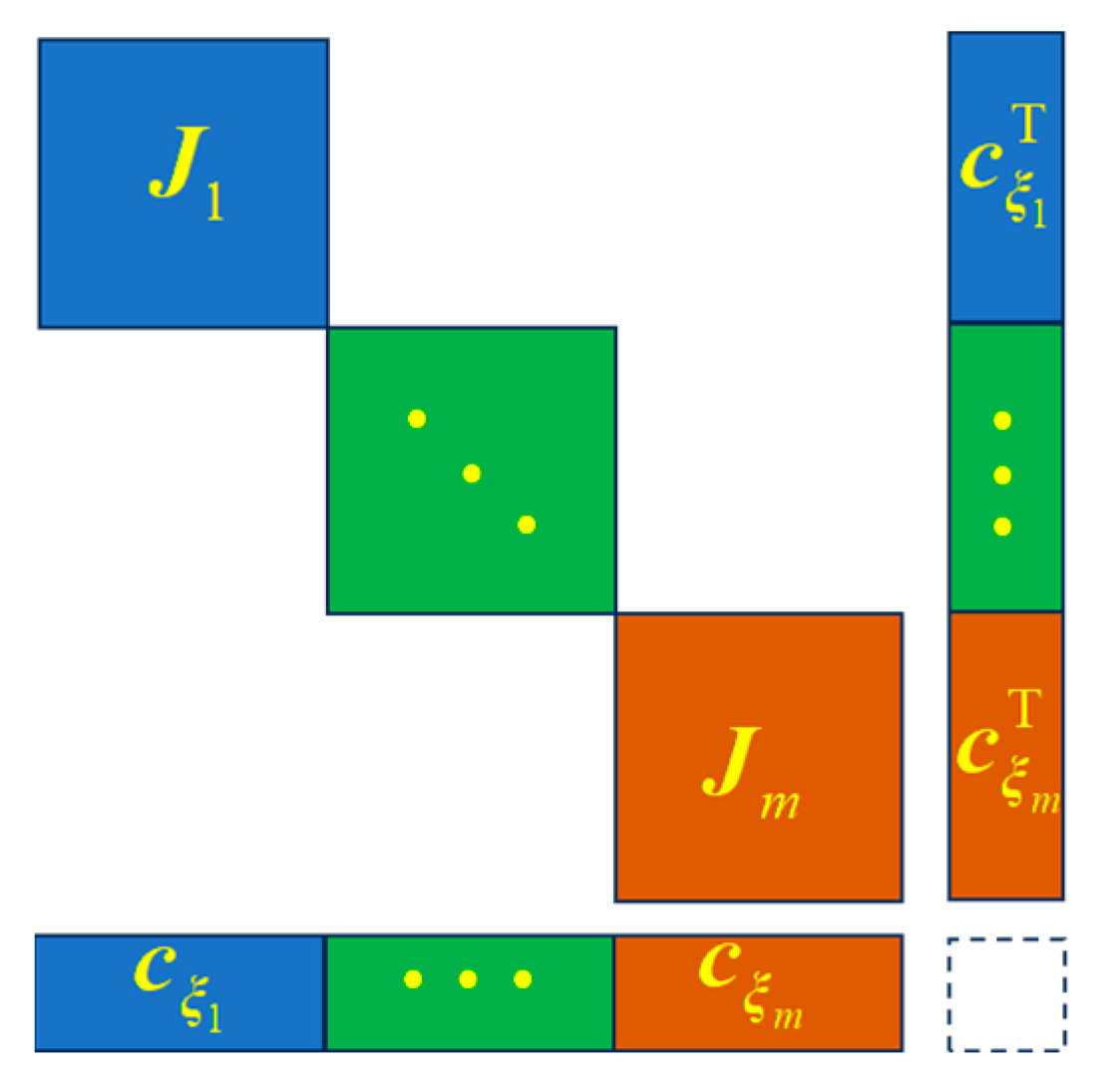
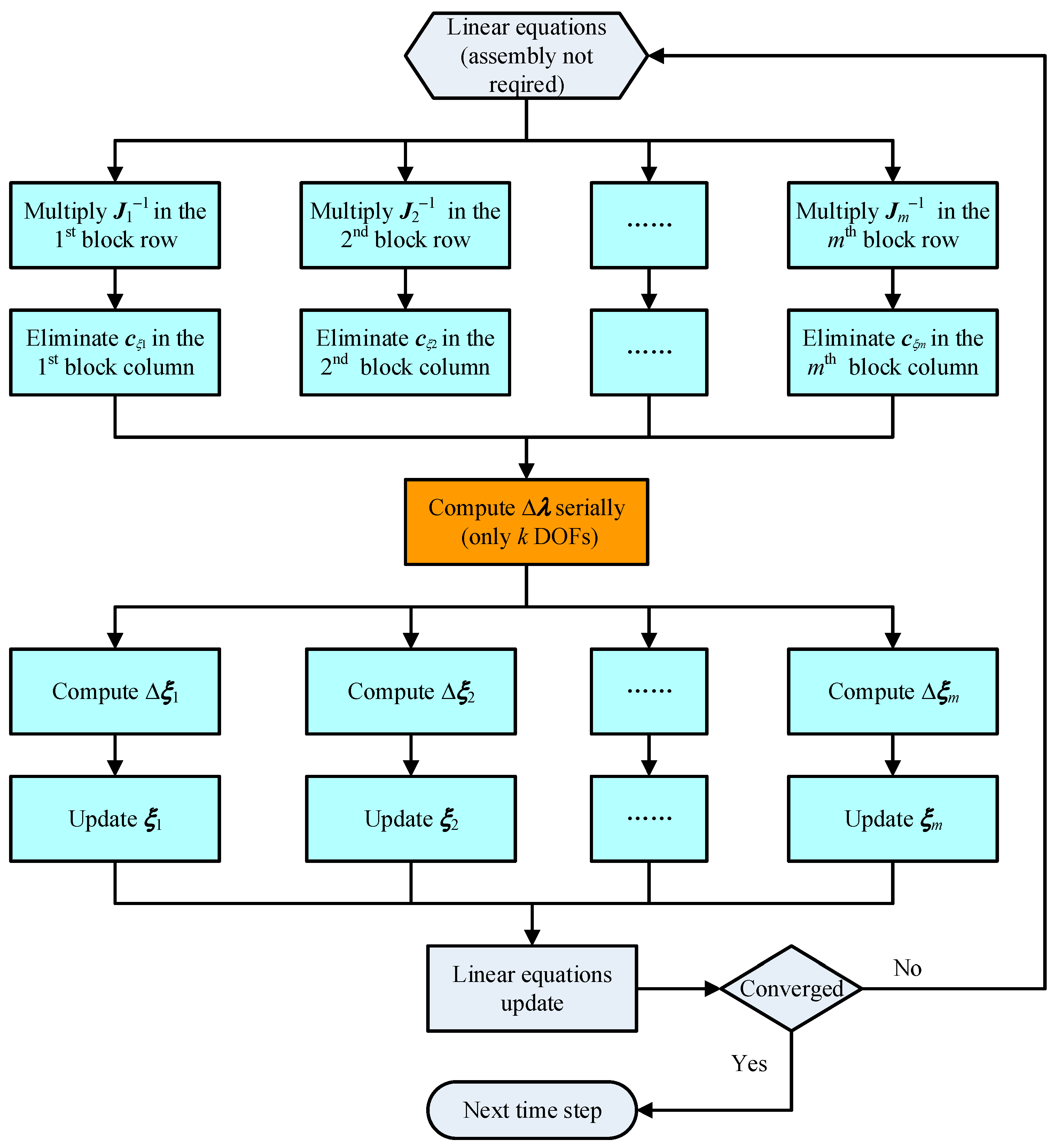
3.3. Algorithm-Level Parallel Direct Solution of System Linear Equations Based on BGE

The block sparsity and symmetry of system Jacobian matrix $J$ resemble that of submatrix $J_i$, which exhibits a strong principal diagonal property as shown in Figure 2 and Figure 3a. Hypothesizing that high-speed rotating parts are not directly incorporated into the system, the Jacobian matrix can still remain positive. This is because damping typically does not dominate the behavior of structural components [29]. Consequently, for the linearized system Equation (45), block Gaussian elimination (BGE) can be employed directly to enable algorithm-level parallel computation.

For convenience, we note $c_{{\xi }_1}\triangleq {\displaystyle \frac{\partial c}{\partial {\xi }_1^{\mathrm{T}}}}$, $c_{{\xi }_1}^{\mathrm{T}}\triangleq {\displaystyle \frac{\partial c^{\mathrm{T}}}{\partial {\xi }_1}}$ and write Equation (45) in a partitioned form as [37] does; thus, we obtain

$$\left[\begin{array}{ccccc}{J}_1& & & & c_{{\xi }_1}^{\mathrm{T}}\\ & J_2& & & c_{{\xi }_2}^{\mathrm{T}}\\ & & \ddots & & ⋮\\ & & & J_m& c_{{\xi }_m}^{\mathrm{T}}\\ c_{{\xi }_1}& c_{{\xi }_2}& \cdots & c_{{\xi }_m}& \end{array}\right]\left[\begin{array}{c}\Delta {\xi }_1\\ \Delta {\xi }_2\\ ⋮\\ \Delta {\xi }_m\\ \Delta \lambda \end{array}\right]=-\left[\begin{array}{c}{\tau }_1\\ {\tau }_2\\ ⋮\\ {\tau }_m\\ c\end{array}\right].$$

(51)

Then, the algorithm-level parallel scheme for the direct solution of the flexible multibody system based on BGE is as follows:

• Step ①: Each block row corresponding to the submatrix $J_i$ is left-multiplied by the Gaussian eliminator $J_i^{-1}$ in parallel to obtain

  $$\left[\begin{array}{ccccc}{E}_{n_1}& & & & J_1^{-1}{c}_{{\xi }_1}^{\mathrm{T}}\\ & E_{n_2}& & & J_2^{-1}{c}_{{\xi }_2}^{\mathrm{T}}\\ & & \ddots & & ⋮\\ & & & E_{n_m}& J_m^{-1}{c}_{{\xi }_m}^{\mathrm{T}}\\ c_{{\xi }_1}& c_{{\xi }_2}& \cdots & c_{{\xi }_m}& \end{array}\right]\left[\begin{array}{c}\Delta {\xi }_1\\ \Delta {\xi }_2\\ ⋮\\ \Delta {\xi }_m\\ \Delta \lambda \end{array}\right]=-\left[\begin{array}{c}{J}_1^{-1}{\tau }_1\\ J_2^{-1}{\tau }_2\\ ⋮\\ J_2^{-1}{\tau }_m\\ c\end{array}\right];$$

  (52)
• Step ②: Each constraint Jacobian matrix $c_{{\xi }_i},\hspace{0.33em}i=1,\cdots ,n_i$ in the lower-left is eliminated in parallel by the unit matrix $E_{n_i}$ in the top-left, resulting in the Schur’s complement $-{\displaystyle \sum _{i=1}^m{c}_{{\xi }_i}{J}_i^{-1}{c}_{{\xi }_i}^{\mathrm{T}}}$ in the subspace of Lagrange multiplier $\lambda$, thus forming

  $$\left[\begin{array}{ccccc}{E}_{n_1}& & & & J_1^{-1}{c}_{{\xi }_1}^{\mathrm{T}}\\ & E_{n_2}& & & J_2^{-1}{c}_{{\xi }_2}^{\mathrm{T}}\\ & & \ddots & & ⋮\\ & & & E_{n_m}& J_m^{-1}{c}_{{\xi }_m}^{\mathrm{T}}\\ & & & & -{\displaystyle \sum _{i=1}^m{c}_{{\xi }_i}{J}_i^{-1}{c}_{{\xi }_i}^{\mathrm{T}}}\end{array}\right]\left[\begin{array}{c}\Delta {\xi }_1\\ \Delta {\xi }_2\\ ⋮\\ \Delta {\xi }_m\\ \Delta \lambda \end{array}\right]=-\left[\begin{array}{c}{J}_1^{-1}{\tau }_1\\ J_2^{-1}{\tau }_2\\ ⋮\\ J_2^{-1}{\tau }_m\\ c-{\displaystyle \sum _{i=1}^m{c}_{{\xi }_i}{J}_i^{-1}{\tau }_i}\end{array}\right];$$

  (53)
• Step ③: The linear equations within the Lagrange multiplier subspace are solved to obtain the multiplier increment as

  $$\Delta \lambda ={\left({\displaystyle \sum _{i=1}^m{c}_{{\xi }_i}{J}_i^{-1}{c}_{{\xi }_i}^{\mathrm{T}}}\right)}^{-1}\left(c-{\displaystyle \sum _{i=1}^m{c}_{{\xi }_i}{J}_i^{-1}{\tau }_i}\right);$$

  (54)
• Step ④: Substitute $\Delta \lambda$ back into Equation (53) to obtain the increments $\Delta {\xi }_i,i=1,\cdots ,m$ in parallel for all bodies. With the known $J_i^{-1}{\tau }_i$ and $J_i^{-1}{c}_{{\xi }_i}^{\mathrm{T}}$ in Step ②, general coordinate increments of bodies are

  $$\Delta {\xi }_i=-J_i^{-1}{\tau }_i-J_i^{-1}{c}_{{\xi }_i}^{\mathrm{T}}\Delta \lambda ,\hspace{0.33em}i=1,\cdots ,m;$$

  (55)
• Step ⑤: Update the general coordinates by the residual increments in parallel for all bodies and constraints. Since the time step $n$ and the iteration superscript $j$ are omitted in Formulas (51)–(55), we restore it to update the Newton iteration as

  $$\left\{\begin{array}{l}{\xi }_i^{(n,j+1)}={\xi }_i^{(n,j)}+\Delta {\xi }_i^{(n,j)}\\ {\lambda }^{(n,j+1)}={\lambda }^{(n,j)}+\Delta {\lambda }^{(n,j)}\end{array}\right..$$

  (56)

In our proposed scheme, steps ①, ②, ④, and ⑤ are algorithmic-level block parallel, whereas step ③ is serial within the $k$ constraint DOFs. In reality, step ③ still allows for acceleration via parallelism in a single column of row [38], but the efficiency of this parallelism [39] is not as high as that of block parallelism. Figure 4 illustrates the flowchart of the presented computational scheme integrating block parallel.

Figure 4. Flowchart of the proposed BGE-based algorithm-level parallel scheme for direct solution of the flexible multibody systems.

Since the original matrix is sparse and there is no interaction between rows and columns required, the assembly of the system matrix $J$ is actually unnecessary. This approach saves time on topology calculation and data copying of sparse matrices, which is advantageous for parallel implementations of both OpenMP and MPI.

The proposed block-parallel scheme remains stable for a system lacking damping and gyroscopic matrix $C$, and the stability analysis process is akin to that of the linearized submatrix Equation (48) for $J_i$ in Section 3.2. We can also anticipate that the BGE-based scheme will be stable when the damping/gyroscopic forces and their Jacobian matrices are small. Typically, damping forces are small for most mechanical structures, and gyroscopic forces are also small for low-speed rotors. However, bodies with high-speed rotation should not be directly incorporated into the system to ensure the stability. Nevertheless, periodic vibrations transmitted from high-speed rotors are permissible within the system, as they do not affect the system’s Jacobian matrix. Consequently, the method presented is suitable for diagnostic platform systems with large translational displacement and for aeroengine stator systems experiencing high-speed excitation forces.

4. Numerical Examples

In this section, an aeroengine stator system and a low-speed crank-slider mechanism are used as numerical examples. The algorithm’s stability is verified by comparing its numerical accuracy with several other methods [40], and its efficiency is also compared.

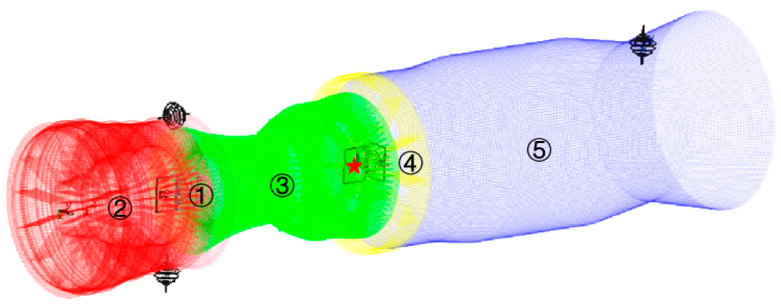
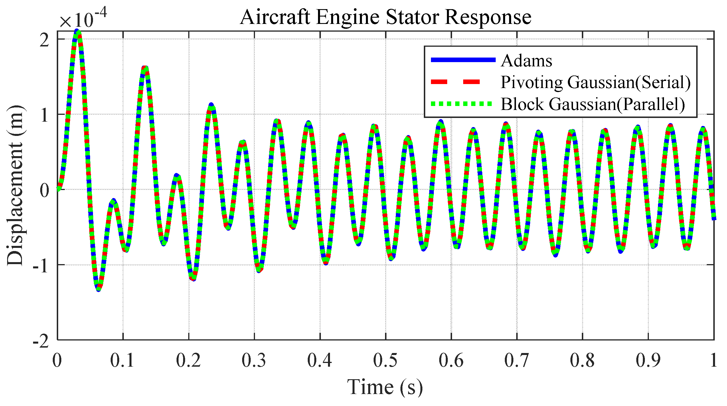
4.1. Example of an Aeroengine Stator System

We consider the vibration response of an aeroengine stator system under the excitation of a rotor’s eccentric periodic force, as depicted in Figure 5. The system comprises five components, a connector, compressor, combustion chamber, turbine, and nozzle, in the order of their modeling (i.e., the sequence of parts in the linearized equations). Each component, treated as an individual entity, is analyzed using finite element software Abaqus 2020 to determine the fixed interface modes, with the lower-order orthogonal elastic modes retained. The part connection relationships, finite element mesh, and number of the CB modes are illustrated in Table 2. A sinusoidal force with a frequency of 20 Hz and an amplitude of 100,000 Newtons is applied at the same position of the fixed connection between part ③ and part ④ (i.e., at the red star point) to simulate the excited vibration of the stator system by the eccentric rotor through the bearing.

Figure 5. Example of an aeroengine stator system: its structural composition, finite element meshing, constraint connections, and position of acting forces.

Table 2. Elastic modal DOFs and constraint connections between components in the aeroengine stator system example.

Part Number (in Order of Assembly)	Part Name	Total Number of the CB Modes	Connections with Other Components
①	Connector	50	(Ball hinge to ground) × 2
②	Compressor	32	Fixed to ①
③	Combustion chamber	26	Fixed to ②
④	Turbine	32	Fixed to ③
⑤	Nozzle	26	Ball hinge to ground

The topology of the Jacobian matrix derived from the aeroengine stator system is depicted in Figure 6. We can observe very appealing block sparsity in the submatrices and the whole matrix, which exhibit self-similarity.

Figure 6. Block sparsity and self-similarity of the Jacobian matrix derived from the aeroengine stator system (nz = none zeros).

For the purpose of comparing accuracy and verifying stability, the numerical results of the aeroengine stator system were computed using the present method, commercial software ADAMS 2020, and the traditional serial Gaussian algorithm. The results are compared in Figure 7, which shows highly consistent outcomes, thereby verifying the numerical stability of the proposed BGE-based algorithm-level parallel method.

Figure 7. Numerical accuracy comparison of the elastic vibration displacement to verify numerical stability of the presented algorithm-level parallel method (using the aeroengine stator system as an example).

As shown in Table 3, when employing 4-core OpenMP parallelism to solve linear Equation (45), the computational efficiency of pivoting GE decreases by 34.7% compared with the serial case, primarily due to the consumption of parallel initialization. This phenomenon illustrates the inadaptability of the pivoting GE to parallelism. In contrast, the efficiency of the block GE parallelism increases by 35.9% compared to its serial counterpart.

Table 3. Computational efficiency comparison between the traditional pivoting GE and the presented parallel BGE method (using the aeroengine stator system as an example).

Method for Solving Equation (45)	Total CPU Time Consumption		Computational Efficiency Improvement by Parallelization 2 (%)	Total Number of Solving System Equation (45)
	Serial (ms)	Parallel with 4 Cores (ms)
Traditional Pivoting GE	666	897	−34.7%	2733
Block GE (presented)	632	405	35.9%	2733
Computational efficiency improvement by block GE 1 (%)	5.1%	54.8%	39.2%	-

¹ Computational efficiency improvement by block GE (%) = (block − pivoting)/pivoting × 100%; ² Computational efficiency improvement by parallelization (%) = (parallel − serial)/serial × 100%.

In the serial case comparison, the block GE efficiency increases by 5.1% compared to the pivoting GE, primarily due to saving of pivoting operations between rows and columns. In contrast, in the parallel case comparison, the block GE efficiency improves by a total of 54.8% over the pivoting GE parallelism. This demonstrates the high parallelism adaptability of the block GE. In summary, the computational efficiency of the presented parallel block GE method increases by 39.2% in total compared to the original serial pivoting GE method.

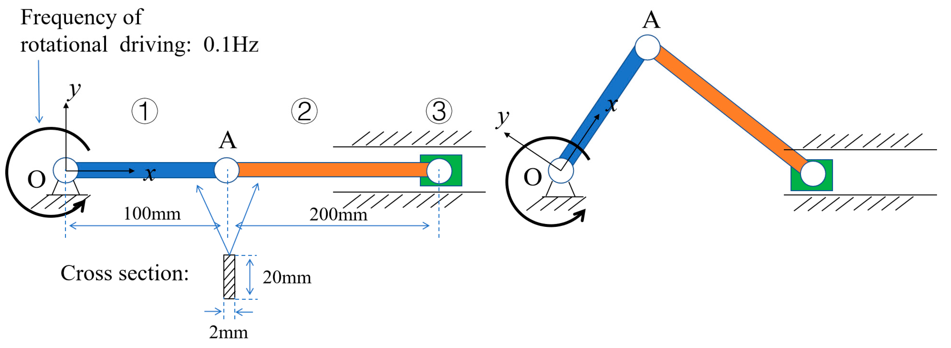
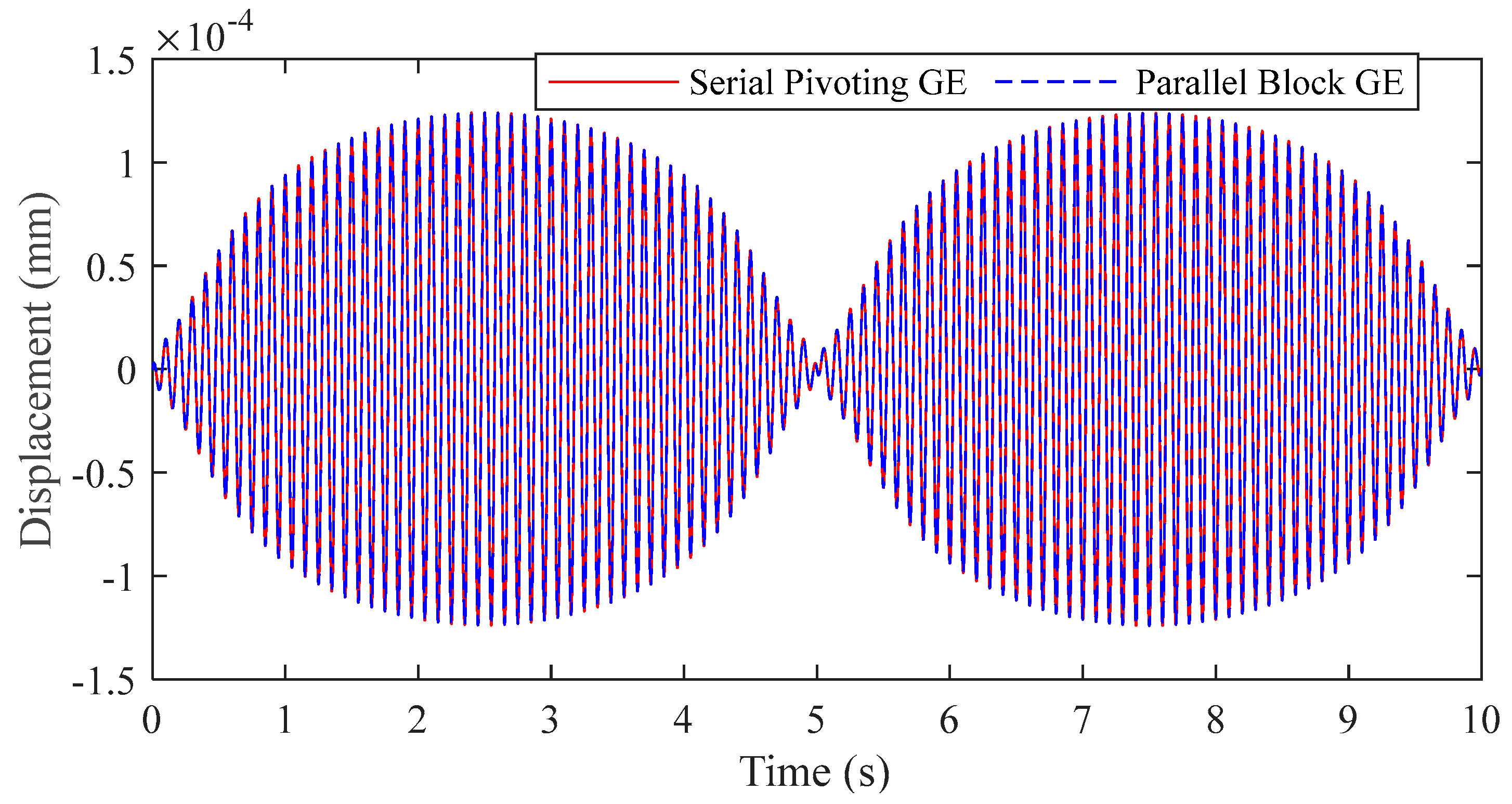
4.2. Sample of a Low-Speed Rotating Crank-Slider Mechanism

Consider the elastic vibration response of a crank-slider mechanism at low speed (0.1 Hz), as depicted in Figure 8. The system consists of a crank, a linker, and a slider, with the elastic DOFs and interconnections detailed in Table 4. The FEM details of the flexible crank and flexible linker for modal analysis are listed in Table 5. We ignore friction in all joints. The physical quantity measured is the elastic displacement of point A in the $y$ direction with respect to the body-fixed coordinate system $\mathrm{O}xy$.

Figure 8. Sample of a low-speed crank-slider mechanism: its components, constraint connections, and rotational driving.

Table 4. Elastic modal DOFs and constraint connections between components in the low-speed crank-slider mechanism.

Part Number (in Order of Assembly)	Part Name	Total Number of the CB Modes	Connections with Other Components
①	Crank	50	Rotation to ground
②	Linker	50	Spin to ①, Spin to ③
③	Slider	0	Translation to ground

Table 5. FEM details of the flexible crank and flexible linker for modal analysis.

FEM Model Item	Value	Note
Material	Aluminum
Density	2700 kg/m3	2.7 × 10−6 tonne/mm3.
Young’s modulus	70 GPa	7 × 104 MPa
Poisson’s ratio	0.3
Finite element size	1 mm × 1 mm × 1 mm	For both the crank and linker
Finite element type	C3D8R	Three-dimensional 8 nodes hexahedral element with reduced integration

The parallel block GE and the serial pivoting GE methods are executed for computational comparison. The elastic part of the vibration response $y_{\mathrm{A}}$, which is the vibration displacement of point A in the body-fixed coordinate system $\mathrm{O}xy$, within one period is shown in Figure 9. The results from both methods are highly coincident, which verifies the numerical stability of the presented parallel block GE method for the FMB system with low-speed rotating parts.

Figure 9. Numerical accuracy comparison of the elastic vibration displacement to verify numerical stability of the presented algorithm-level parallel method (using the low-speed crank-slider mechanism as a sample).

As indicated in Table 6, the overall computational efficiency increased by 1.9% in the low-speed crank-slider sample, where the total CPU time consumption decreased from 4089 ms to 4013 ms. The parallelization of the presented block GE method accelerates the FMB system with low-speed rotating parts, albeit not to the extent demonstrated in the example of the aeroengine stator system. This is due to the presence of five flexible components in the aeroengine example compared to only two in the current crank-slider sample. This phenomenon suggests that the parallelization efficiency of the presented method is related to the number of flexible components in the system. In other words, the parallelization is executed between sub-blocks of flexible components.

Table 6. Computational efficiency comparison between the serial pivoting GE method and the presented parallel block GE method (using the low-speed crank-slider mechanism as a sample).

Method for Solving Equation (45)	Total CPU Time Consumption (ms)	Total Number of Solving System Equation (45)
Serial pivoting GE	4089	30,214
Parallel block GE (presented, with 4 cores OpenMP)	4013	31,546
Computational efficiency improvement by block GE (%) 1	1.9%	-

¹ Computational efficiency improvement by block GE (%) = (block − pivoting)/pivoting × 100%.

It is also noteworthy that the number of solving the linearized systemic Equation (45) rose from 30,214 to 31,546, an increase of approximately 4.4%. This is due to the fact that the gyroscopic component of the Jacobian matrix $C$ is neglected in Equation (45) using our method. This results in the Newton iteration degenerating into the quasi-Newton iteration, which typically requires more iterations in engineering applications. Consequently, despite a 4.4% increase in the total number of iterations, a computational efficiency improvement of 1.9% is realized. As previously analyzed, the parallel efficiency can be significantly enhanced in scenarios involving more elastic modes or more flexible components within the FMB systems in question.

5. Conclusions

In this paper, the CB method is utilized to model large, complex, flexible, multibody systems. System Jacobian matrices with favorable block symmetry and sparsity properties are formed by appropriately ordering the generalized coordinates of bodies and joints. A local–global two-layer parallel algorithm is constructed to directly solve the linearized systemic equations. The algorithm also circumvents the disruption of matrix topological sparsity in the traditional pivoting GE process of direct solution and achieves algorithm-level parallelism. The algorithm ensures numerical stability by employing the physical assumption of component modal synthesis methods and the specific format of the Craig–Bampton method. The numerical stability and high efficiency of the proposed block parallel algorithm are validated by comparing the results with those from commercial software Abaqus 2020 and with the pivoting GE algorithm, using the examples of aeroengine stator system vibration and crank-slider mechanism’s low-speed rotation.

The method detailed in this paper is unsuitable for multibody systems that contain high-speed rotating parts directly, as in such cases, the gyroscopic matrix may become the primary component of the Jacobi matrix, leading to instability in the presented scheme. A potential solution is to construct an appropriate preconditioning matrix [40] to ensure numerical stability and prevent the need for pivoting operations. This approach could be explored in future papers.

References

- Simeon, B. Computational Flexible Multibody Dynamics. A Differential-Algebraic Approach; Springer: Berlin/Heidelberg, Germany, 2013. [Google Scholar]
- Shabana, A.A. Dynamics of Multibody Systems; Wiley: New York, NY, USA, 1989. [Google Scholar]
- Craig, R.R.J. Substructure methods in vibration. J. Mech. Des. 1995, 117, 207–213. [Google Scholar] [CrossRef]
- Song, J.O.; Haug, E.J. Dynamic analysis of planar flexible mechanisms. Comput. Methods Appl. Mech. Eng. 1980, 24, 359–381. [Google Scholar] [CrossRef]
- Hurty, W.C. Dynamic analysis of structural systems using component modes. AIAA J. 1965, 3, 678–685. [Google Scholar] [CrossRef]
- Bampton, M.C.C.; Craig, J.R.R. Coupling of substructures for dynamic analyses. AIAA J. 1968, 6, 1313–1319. [Google Scholar]
- Hou, S.N. Review of Modal Synthesis Techniques and a New Approach; NASA: Washington, DC, USA, 1969. [Google Scholar]
- Macneal, R.H. A hybrid method of component mode synthesis. Comput. Struct. 1971, 1, 581–601. [Google Scholar] [CrossRef]
- Rubin, S. Improved component-mode representation for structural dynamic analysis. AIAA J. 1975, 13, 995–1006. [Google Scholar] [CrossRef]
- Kim, J.G.; Lee, P.S. An enhanced craig–bampton method. Int. J. Numer. Methods Eng. 2015, 103, 79–93. [Google Scholar] [CrossRef]
- Kim, J.G.; Park, Y.J.; Lee, G.H.; Kim, D.N. A general model reduction with primal assembly in structural dynamics. Comput. Methods Appl. Mech. Eng. 2017, 324, 1–28. [Google Scholar] [CrossRef]
- Kim, J.G.; Han, J.B.; Lee, H.; Kim, S.S. Flexible multibody dynamics using coordinate reduction improved by dynamic correction. Multibody Syst. Dyn. 2018, 42, 411–429. [Google Scholar] [CrossRef]
- Han, J.B.; Kim, J.G.; Kim, S.S. An efficient formulation for flexible multibody dynamics using a condensation of deformation coordinates. Multibody Syst. Dyn. 2019, 47, 293–316. [Google Scholar] [CrossRef]
- Wanner, G.; Hairer, E. Solving Ordinary Differential Equations II; Springer: Berlin/Heidelberg, Germany; New York, NY, USA, 1996; Volume 375. [Google Scholar]
- Yang, C.; Du, J.; Cheng, Z.; Wu, Y.; Li, C. Flexibility investigation of a marine riser system based on an accurate and efficient modelling and flexible multibody dynamics. Ocean Eng. 2020, 207, 107407. [Google Scholar] [CrossRef]
- Park, K.C.; Downer, J.D.; Chiou, J.C.; Farhat, C. A modular multibody analysis capability for high-precision, active control and real-time applications. Int. J. Numer. Methods Eng. 1991, 32, 1767–1798. [Google Scholar] [CrossRef]
- Cao, D.Z.; Qiang, H.F.; Ren, G.X. Parallel computing studies of flexible multibody system dynamics using OpenMP and Pardiso. J. Tsinghua Univ. Sci. Technol. 2012, 52, 1643–1649. [Google Scholar]
- Dagum, L.; Menon, R. OpenMP: An industry standard API for shared-memory programming. J. IEEE Comput. Sci. Eng. 1998, 5, 46–55. [Google Scholar] [CrossRef]
- Negrut, D.; Tasora, A.; Mazhar, H.; Heyn, T.; Hahn, P. Leveraging parallel computing in multibody dynamics. Multibody Syst. Dyn. 2012, 27, 95–117. [Google Scholar] [CrossRef]
- Negrut, D.; Serban, R.; Mazhar, H.; Heyn, T. Parallel computing in multibody system dynamics: Why, when, and how. J. Comput. Nonlinear Dyn. 2014, 9, 041007. [Google Scholar] [CrossRef]
- Pařík, P.; Kim, J.G.; Isoz, M.; Ahn, C.U. A parallel approach of the enhanced Craig–Bampton method. Mathematics 2021, 9, 3278. [Google Scholar] [CrossRef]
- Cros, J.M. Parallel modal synthesis methods in structural dynamics. Contemp. Math. 1998, 218, 492–499. [Google Scholar]
- Murthy, P.; Poschmann, P.; Reymond, M.; Schartz, P.; Wilson, C.T. Automated Component Modal Synthesis with Parallel Processing. 2000. Available online: http://www.mscsoftware.com/support/library/conf/auto00/p03900.pdf (accessed on 22 October 2024).
- Li, P.; Liu, C.; Tian, Q.; Hu, H.Y.; Song, Y.P. Dynamics of a deployable mesh reflector of satellite antenna: Parallel computation and deployment simulation. J. Comput. Nonlinear Dyn. 2016, 11, 061005. [Google Scholar] [CrossRef]
- Featherstone, R. A divide-and-conquer articulated-body algorithm for parallel O(log(n)) calculation of rigid-body dynamics. Part 1: Basic algorithm. Int. J. Robot. Res. 1999, 18, 876–892. [Google Scholar] [CrossRef]
- Dewes, E.M.; Rixen, D.J. Time integration of multibody systems using nonlinear domain decomposition techniques with mixed interface conditions. In Proceedings of the 5th Joint International Conference on Multibody System Dynamics, Lisboa, Portugal, 24–28 June 2018. [Google Scholar]
- Cano, J.C.; Cuenca, J.; Giménez, D.; Saura-Sánchez, M.; Segado-Cabezos, P. A parallel simulator for multibody systems based on group equations. J. Supercomput. 2019, 75, 1368–1381. [Google Scholar] [CrossRef]
- Wasfy, T.M.; Noor, A.K. Computational strategies for flexible multibody systems. Appl. Mech. Rev. 2003, 56, 553–613. [Google Scholar] [CrossRef]
- Higham, N.J. Gaussian elimination. Wiley Interdiscip. Rev. Comput. Stat. 2011, 3, 230–238. [Google Scholar] [CrossRef]
- Peiret, A.; Andrews, S.; Kövecses, J.; Kry, P.G.; Teichmann, M. Schur complement-based substructuring of stiff multibody systems with contact. ACM Trans. Graph. 2019, 38, 1–17. [Google Scholar] [CrossRef]
- Yang, C.; Cao, D.Z.; Zhao, Z.H.; Zhang, Z.R.; Ren, G.X. A direct eigenanalysis of multibody system in equilibrium. J. Appl. Math. 2012, 2012, 1–7. [Google Scholar] [CrossRef]
- Wang, G.X.; Niu, Z.P.; Feng, Y. Improved Craig–Bampton Method Implemented into Durability Analysis of Flexible Multibody Systems. Actuators 2023, 12, 65. [Google Scholar] [CrossRef]
- Ryan, R.R. ADAMS—Multibody system analysis software. In Multibody Systems Handbook; Springer: Berlin/Heidelberg, Germany, 1990; pp. 361–402. [Google Scholar]
- Pan, V.Y.; Zhao, L. Numerically safe Gaussian elimination with no pivoting. Linear Algebra Its Appl. 2017, 527, 349–383. [Google Scholar] [CrossRef]
- Strawderman, R.L.; Higham, N.J. Accuracy and stability of numerical algorithms. J. Am. Stat. Assoc. 1999. [Google Scholar] [CrossRef]
- Bender, J.; Erleben, K.; Trinkle, J. Interactive simulation of rigid body dynamics in computer graphics. Comput. Graph. Forum 2014, 33, 246–270. [Google Scholar] [CrossRef]
- Golub, G.H.; Greif, C. On solving block-structured indefinite linear systems. SIAM J. Sci. Comput. 2003, 24, 2076–2092. [Google Scholar] [CrossRef]
- Faugère, J.C.; Lachartre, S. Parallel Gaussian elimination for Gröbner bases computations in finite fields. In Proceedings of the International Workshop on Parallel Symbolic Computation, Grenoble, France, 21–23 July 2010. [Google Scholar]
- Peng, R.; Vempala, S. Solving sparse linear systems faster than matrix multiplication. In Proceedings of the Symposium on Discrete Algorithms, Virtual, 10–13 January 2021. [Google Scholar]
- Sewell, G. Computational Methods of Linear Algebra; World Scientific Publishing Company: Singapore, 2014. [Google Scholar]
Disclaimer/Publisher’s Note: The statements, opinions and data contained in all publications are solely those of the individual author(s) and contributor(s) and not of MDPI and/or the editor(s). MDPI and/or the editor(s) disclaim responsibility for any injury to people or property resulting from any ideas, methods, instructions or products referred to in the content. |
© 2025 by the authors. Licensee MDPI, Basel, Switzerland. This article is an open access article distributed under the terms and conditions of the Creative Commons Attribution (CC BY) license (https://creativecommons.org/licenses/by/4.0/).