In Silico Methods for Assessing Cancer Immunogenicity—A Comparison Between Peptide and Protein Models

Abstract

Identifying and characterizing putative tumor antigens is essential to cancer vaccine development. Given the impracticality of isolating and evaluating each potential antigen individually, in silico prediction algorithms, especially those employing machine learning (ML) techniques, are indispensable. These algorithms substantially decrease the experimental workload required for discovering viable vaccine candidates, thereby accelerating the development process and enhancing the efficiency of identifying promising immunogenic targets. In this study, we employed six supervised ML methods on a dataset containing 546 experimentally validated immunogenic human tumor proteins and 548 non-immunogenic human proteins to develop models for immunogenicity prediction. These models included k-nearest neighbor (kNN), linear discriminant analysis (LDA), quadratic discriminant analysis (QDA), support vector machine (SVM), random forest (RF), and extreme gradient boosting (XGBoost). After validation through internal cross-validation and an external test set, the best-performing models (QDA, RF, and XGBoost) were selected for further evaluation. A comparison between the chosen protein models and our previously developed peptide models for tumor immunogenicity prediction revealed that the peptide models slightly outperformed the protein models. However, since both proteins and peptides can be subject to tumor immunogenicity assessment, evaluating each with the respective models is prudent. The three selected protein models are set to be integrated into the new version of the VaxiJen server.

1. Introduction

Peptide-based cancer vaccines are emerging as pivotal in the treatment of human tumors. They instruct the immune system to recognize tumor antigens as foreign [1]. When capable of eliciting a sufficient immune response that leads to the formation of memory cells, these antigens are classified as protective immunogens. This ability to provoke an enduring immune response is crucial for the effectiveness of cancer vaccines in providing long-term protection against tumor recurrence.

Identifying suitable antigens is crucial in developing peptide cancer vaccines [2]. In the ideal situation, each potential antigen would be isolated or synthesized, and then its immunogenic qualities would be empirically evaluated. However, this strategy is hampered by several practical and logistical issues, such as the difficulty of replicating human immune responses in experimental settings, expensive expenditures, and time-consuming laboratory processes. Another significant challenge is that, to date, the pool of experimentally confirmed tumor antigens remains relatively small. Although plenty of in vitro validated data and animal studies performed in vivo, the direct applicability of these findings to human cancer patients is not straightforward due to the complex nature of the human immune system. In silico prediction algorithms can address both of these problems. By leveraging known experimentally confirmed immunogens, classification models that distinguish them from the non-immunogenic ones can be derived, significantly reducing the need for biological assessment of every putative immunogen. Thus, in silico prediction algorithms have emerged as innovative tools by rationalizing the antigen discovery process in recent years [3].

Such models have already proven to be robust [4,5,6,7]. Our recent work utilized many machine-learning methods to develop models for classifying immunogenic human tumor peptides [8]. The present study aims to train similar algorithms on a dataset of whole proteins and to compare the observed results. The models with the best performance metrics are projected to be implemented in the third version of the VaxiJen web server.

VaxiJen is the first server to offer an alignment-independent prediction of protective antigens from viral, bacterial, parasite, fungal, and tumor origin [9]. Identifying tumor antigens uses two distinct datasets, each containing 100 well-known antigens and 100 known non-antigens, each being a whole protein molecule. The method employs a machine learning approach where each protein is represented as a string of z-scales [10], which capture the main physicochemical properties of the amino acid residues. These strings are converted into uniform vectors using auto-cross covariance (ACC) [11]. A genetic algorithm (GA) [12] is used to identify relevant variables within these vectors. Finally, partial least squares-based discriminant analysis (PLS-DA) [13] is used to develop the prediction model.

2. Materials and Methods

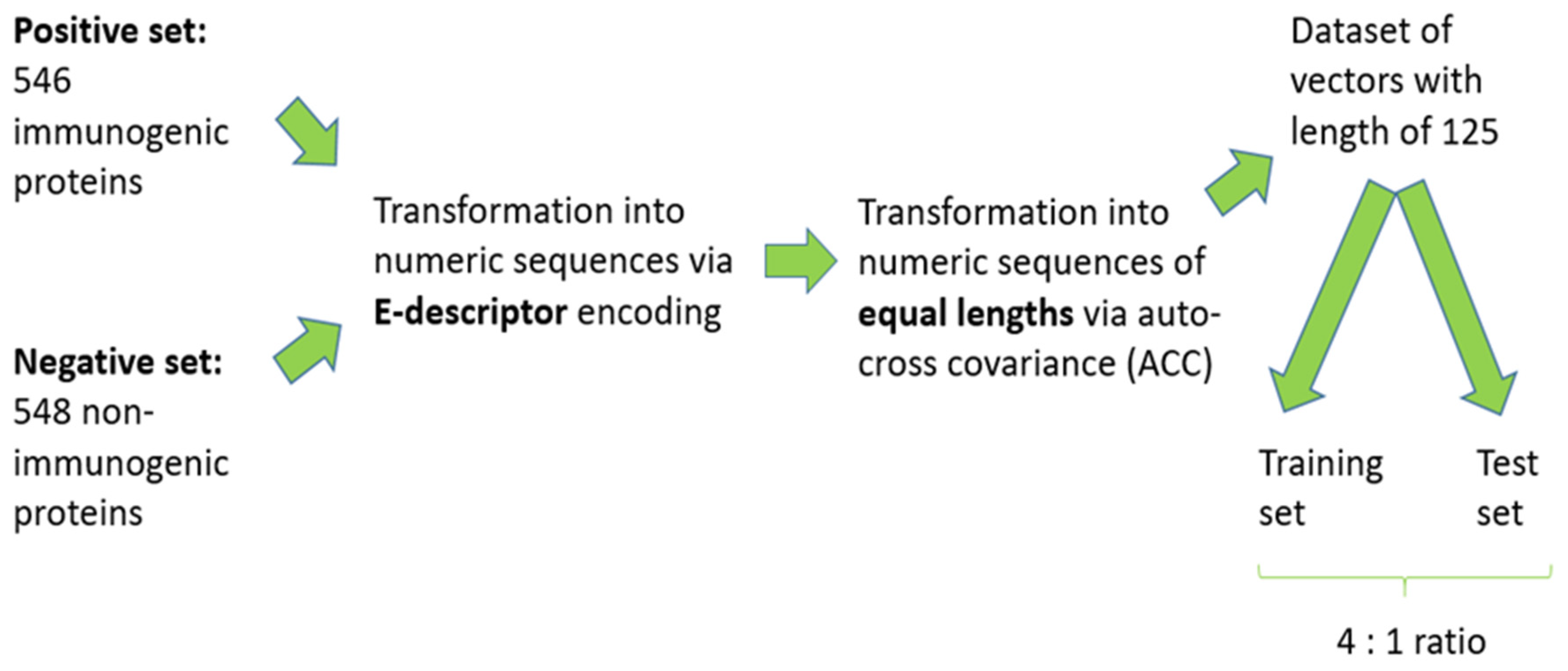
2.1. Datasets

A thorough search was conducted in the U.S. National Library of Medicine’s PubMed database to find publications on immunogenic proteins, focusing solely on human studies. The search settings used were: (cancer OR tumor OR tumour) AND (candidate OR candidates OR subunit) AND (protects OR protect OR protection OR protective) AND (vaccine OR vaccines). Moreover, the built-in Similar Articles tool within PubMed was employed for an expanded exploration of the relevant literature. The publications were manually curated, and information about experimentally determined human cancer antigens was obtained. A dataset of sequences of the selected immunogenic proteins in FASTA format was obtained and compiled via UniProtKB, the central hub for collecting functional protein information.

A corresponding dataset of non-immunogenic proteins was compiled by performing a BLAST (ncbi-blast-2.15.0+) search of proteins from the human proteome against the identified immunogenic proteins to select similar sequences. The absence of immunogenicity was verified by using the VaxiJen 2.0 web server (https://www.ddg-pharmfac.net/vaxijen/VaxiJen/VaxiJen.html (accessed on 7 April 2025), Medical University-Sofia, Sofia, Bulgaria). Detailed information about the UniProt identification numbers, links to the UniProt entry, references, and PubMed identification numbers for each positive and negative protein used in the study are presented in Tables S3.1 and S3.2 in the Supplementary Materials.

The gathered dataset of immunogenic and non-immunogenic proteins was randomized, and 20% was designated as a test set for the subsequent validation of the derived models.

2.2. Descriptors

In this study, E-descriptors were used to characterize protein sequences quantitatively. These descriptors, introduced by Venkatarajan and Braun, assign five numerical values to each of the 20 naturally occurring amino acids through multidimensional scaling of 237 physicochemical properties [14]. The first component, E1, strongly correlates with amino acid hydrophobicity, while E2 provides information on molecular size and steric properties. The presence of amino acids in α-helices and β-strands is indicated by components E3 and E5, respectively. The E4 component considers the relative frequency of amino acids in proteins, the number of codons, and partial specific volume. A string of 5n elements, where n is the protein length, represents each protein in the dataset. Because these strings differ in size, auto- and cross-covariance (ACC) transformation was used to convert them into uniform vectors.

2.3. Auto-Cross Covariance (ACC) Transformation

Wold et al. introduced the auto- and cross-covariance transformation of protein sequences in 1993 [11]. Polypeptide chains of varying lengths are converted into uniform, equal-length vectors using this alignment-independent preprocessing method. A key advantage of ACC is its ability to account for interactions between neighboring residues, capturing sequence-order effects. Auto- and cross-covariance are calculated via the following specific formulas:

$$AC{C}_{j,j}\left(L\right)={\sum }_i^{n-L}{\displaystyle \frac{E_{j,i}\times E_{j,i+L}}{n-L}}$$

(1)

$$AC{C}_{j,k}\left(L\right)={\sum }_i^{n-L}{\displaystyle \frac{E_{j,i}\times E_{k,i+L}}{n-L}}$$

(2)

where:

• E—E-descriptor value
• j, k (j ≠ k)—number of the E-descriptor (j, k = 1–5)
• i—position of amino acid in the peptide chain (i = 1, 2, 3…n)
• n—number of amino acids in the protein
• L—lag-value: the length of the frame of the contiguous amino acids

2.4. Machine Learning Methods

In this study, several machine learning (ML) approaches were employed, as described in the following sections. All models were implemented using Python 3.7 and the scikit-learn library [15]. To optimize performance, hyperparameter tuning was conducted via Grid Search [16], which systematically evaluates combinations of parameters within a predefined search space. The best-performing hyperparameters for each model are provided in Supplementary File S2, Table S2. The models were trained on auto- and cross-covariance (ACC)-transformed amino acid sequences to classify proteins as immunogenic (output = 1) or non-immunogenic (output = 0).

2.4.1. k-Nearest Neighbor (kNN)

The idea behind the k-nearest neighbors (kNN) technique is that data points with similar characteristics typically have similar labels or values [17]. The model keeps the entire dataset as a reference library throughout training. The label is assigned based on the majority class among its k nearest neighbors after calculating the distance (such as the Euclidean distance) between the query instance and all stored training examples.

2.4.2. Linear Discriminant Analysis (LDA)

Linear discriminant analysis (LDA) is a supervised learning method that performs both classification and dimensionality reduction [18]. LDA converts the initial D-dimensional feature space into a lower-dimensional subspace (D’, where D > D’) for classification tasks. By increasing inter-class variation and decreasing intra-class variance, this projection seeks to improve class separability.

2.4.3. Quadratic Discriminant Analysis (QDA)

Quadratic discriminant analysis (QDA) shares conceptual similarities with LDA but employs a quadratic decision boundary for class separation [18]. QDA assumes Gaussian-distributed data for every class, in contrast to LDA. Class-specific mean vectors, the average feature values within each class, and class-specific priors, the relative frequency of data points per class, are incorporated into the model.

2.4.4. Support Vector Machine (SVM)

An ideal decision boundary (hyperplane) to differentiate between two classes is identified by the support vector machine (SVM) [19]. Even though there may be more than one separating hyperplane, SVM finds the best answer by maximizing the margin, or the maximum separation between the hyperplane and the nearest data points for each class (support vectors). By establishing the broadest feasible division between classes, this margin maximization strategy improves the model’s capacity for generalization.

2.4.5. Random Forest (RF)

An ensemble learning technique called random forest (RF) aggregates predictions from several decision trees to provide a more reliable and consistent result [20]. By merging several trees, RF reduces overfitting and improves resistance to noisy data and outliers. The final forecast for classification problems equals the majority vote cast by all of the forest’s trees. In regression applications, the model usually calculates the average prediction of all the individual trees.

2.4.6. Extreme Gradient Boosting (XGBoost)

A sophisticated gradient boosting algorithm designed for scalable and high-performance machine learning is extreme gradient boosting (XGBoost) [21]. This ensemble approach builds a series of weak decision trees repeatedly, with each new tree concentrating on using adaptive weighting to fix the residuals of its predecessors. The weighting scheme is established by minimizing a given loss function that measures the difference between expected and actual values. Ultimately, XGBoost creates predictions by combining the outputs of each component tree with precisely calibrated weights in an additive model.

2.5. Machine Learning Models Validation

To ensure the robust evaluation of our machine learning models, we implemented a comprehensive validation approach combining 10-fold cross-validation and independent test set assessment. The cross-validation procedure partitions the training data into 10 distinct subsets (k = 10) [22], iteratively training the model on nine subsets while using the remaining subset for validation. This process repeats until each subset is the validation set once, with final performance metrics representing the average across all iterations. While computationally intensive, this approach optimizes data utilization—particularly valuable for limited datasets—while providing reliable performance estimates. The models were further validated on a completely independent test set to confirm generalizability.

Model performance was evaluated using receiver operating characteristic (ROC) analysis, which quantifies classification outcomes through four metrics: true positives (TP), true negatives (TN), false positives (FP), and false negatives (FN) [23]. We employed multiple evaluation measures:

• Sensitivity: The true positive rate, indicating the model’s capability to identify immunogenic proteins correctly.

$$Sensitivity={\displaystyle \frac{TP}{TP+FN}}$$

(3)

• Specificity: The true negative rate, reflecting accurate detection of non-immunogenic proteins.

$$Specificity={\displaystyle \frac{TN}{TN+FP}}$$

(4)

• Accuracy: The overall classification performance is calculated as the proportion of correct predictions across all samples.

$$Accuracy={\displaystyle \frac{TP+TN}{TP+TN+FP+FN}}$$

(5)

• Area Under the ROC Curve (AUC): Ranging from 0.5 (random chance) to 1.0 (perfect discrimination), assessing overall predictive efficacy.
• Matthew’s Correlation Coefficient (MCC): A balanced measure particularly valuable for imbalanced datasets, where +1 represents perfect prediction, −1 indicates total disagreement, and 0 suggests random classification.

$$MCC={\displaystyle \frac{TP\times TN-FP\times FN}{\sqrt{(TP+FP)(TP+FN)(TN+FP)(TN+FN)}}}$$

(6)

To assess the robustness of our models and verify that predictions were not artifacts of chance correlations, we employed Y-scrambling (also known as label permutation) [24]. This validation procedure consists of (1) training the model on the original dataset and recording its performance metrics, followed by (2) repeatedly shuffling the target labels while maintaining feature values, then retraining and evaluating the model. A robust model should perform significantly better on the original data than the permuted datasets. If the model maintains comparable performance across scrambled datasets with low variance, this suggests the initial predictions may have resulted from random correlations rather than meaningful relationships in the data.

To elucidate the contribution of individual features to model performance, we applied two interpretability techniques to our top-performing models. The scikit-learn library implements the first technique, permutation feature importance. Using this technique, one feature’s values are shuffled randomly, and the model’s score is tracked as it declines. The second method, drop-column feature importance, involves deleting a whole feature column from the dataset, training a new model, and evaluating its performance. The idea behind both approaches is that removing a feature that is not important should not have a significant negative impact on the model’s performance. Features showing minimal effects on model performance when altered or excluded are considered less important for the prediction task.

3. Results

3.1. Data Preprocessing

The PubMed search yielded 6829 articles. They were manually curated, and information about 5199 human cancer antigens was obtained. Among them, only those with experimental data for immunogenicity were collected, resulting in 548 antigenic and immunogenic proteins. In addition to them, following the previously described methodology, 548 antigenic but non-immunogenic proteins were compiled. Thus, the final dataset consisted of 546 immunogenic and 548 non-immunogenic proteins. The dataset was partitioned into balanced training (436 immunogenic and 439 non-immunogenic proteins) and test (110 immunogenic and 109 non-immunogenic proteins) sets. Each protein was encoded as a numerical sequence using 5n E-descriptors, where n represents the amino acid sequence length. We applied auto- and cross-covariance (ACC) transformation with a lag value of L = 5 to handle variable-length sequences, generating fixed-dimensional feature vectors. This processing converted the training set into an 875 × 125 matrix (5 descriptors × 5² autocorrelation terms) and the test set into a 219 × 125 matrix. Figure 1 illustrates the complete data preprocessing pipeline.

3.2. Development and Validation of ML Models

Using the training dataset, we employed six supervised machine learning algorithms to develop immunogenicity classification models. Hyperparameter tuning was conducted via grid search with 10-fold cross-validation to optimize model performance. This exhaustive search evaluated all possible combinations within predefined hyperparameter spaces for each algorithm. The optimal configurations were determined as follows:

• kNN: k = 2 neighbors
• LDA: Singular Value Decomposition solver (svd)
• QDA: Regularization parameter (reg_param) = 0.0
• SVM: Radial basis function kernel (rbf) with C = 50 and γ = 100
• RF: 100 estimators with max_depth = 50 and max_features = 2
• XGBoost: learning_rate = 0.01, max_depth = 7, and 100 estimators

Table 1. Summary of the performance of the ML models on the training set (10-fold cross-validation). AROC—area under the ROC curve (sensitivity vs. 1-specificity); MCC—Matthew’s correlation coefficient.

Algorithm	Sensitivity	Specificity	Accuracy	AROC	MCC
kNN	0.73	0.46	0.60	0.60	0.20
LDA	0.71	0.53	0.62	0.63	0.22
QDA	0.67	0.81	0.74	0.83	0.49
SVM	0.80	0.66	0.73	0.80	0.46
RF	0.71	0.79	0.75	0.82	0.51
XGBoost	0.75	0.75	0.75	0.81	0.50

presents the models’ performance on the training set. Based on the overall performance, we selected QDA, RF, and XGBoost as the most promising algorithms for predicting the immunogenicity of tumor proteins. These models are subject to further validation.

The three selected models were evaluated on an external test set.

Table 2. Comparison of the performance of the best protein and the best peptide models on their respective test sets. AROC—area under the ROC curve (sensitivity vs. 1-specificity); MCC—Matthew’s correlation coefficient.

Algorithm	Sensitivity	Specificity	Accuracy	AROC	MCC
Proteins
QDA	0.63	0.81	0.72	0.82	0.44
RF	0.71	0.79	0.75	0.81	0.50
XGBoost	0.74	0.77	0.75	0.80	0.51
Peptides
SVM	0.79	0.86	0.82	0.83	0.64
RF	0.76	0.93	0.85	0.80	0.70
XGBoost	0.79	0.76	0.77	0.83	0.55

compares their results with the best-performing peptide models highlighted in our previous work.

3.3. ML Models Robustness Assessment

The initial stage of additional validation of the derived models involved Y-scrambling. This process was repeated 100 times for each model, and the average accuracy scores were calculated based on the test set.

Table 3. Comparison of the Y-scrambling analysis on the selected protein and peptide models on their respective test sets.

Algorithm	Accuracy
Proteins
QDA	0.4986
RF	0.4906
XGBoost	0.4975
Peptides
SVM	0.5075
RF	0.5182
XGBoost	0.4987

compares the Y-scrambling results for the three best models for proteins and peptides.

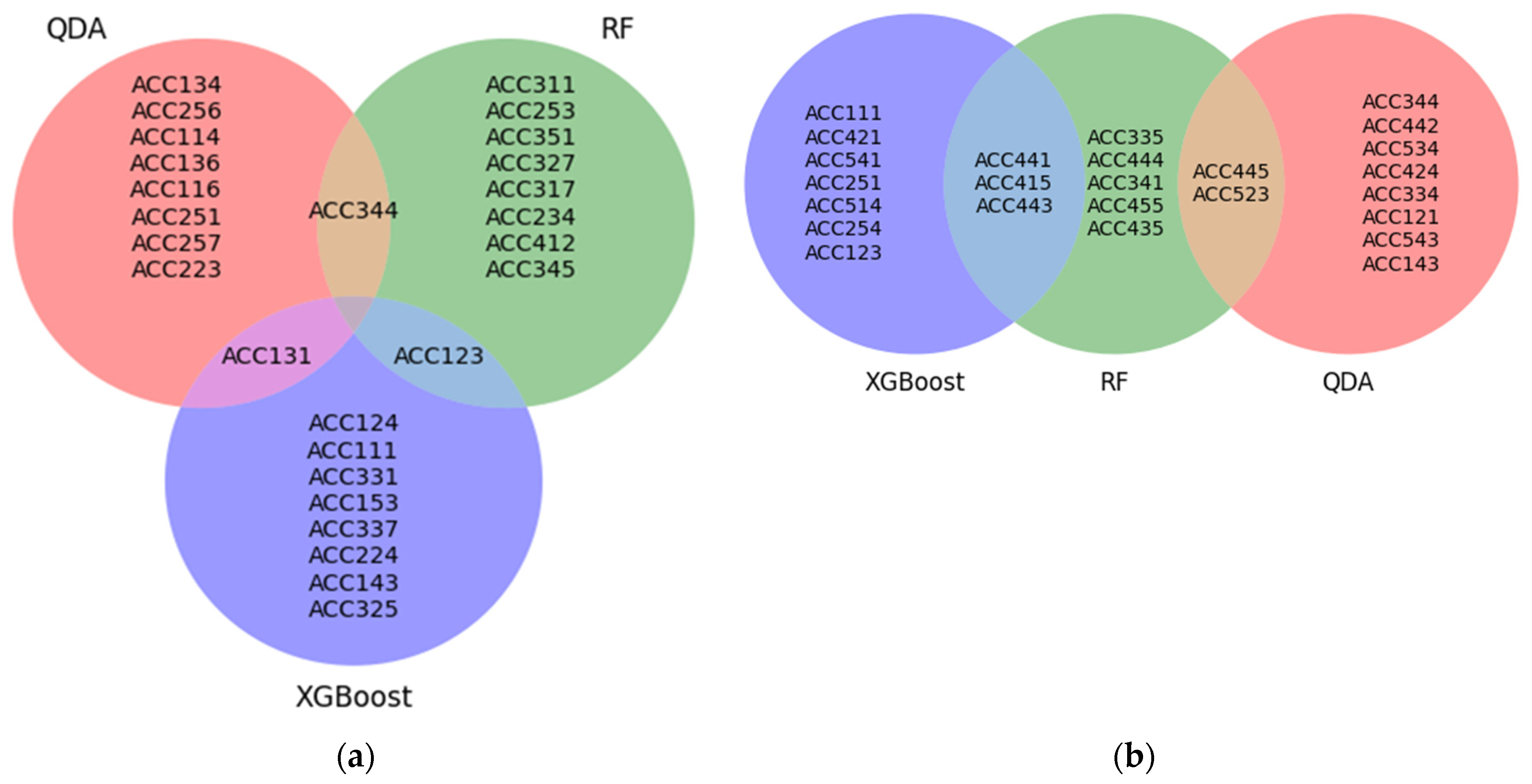
3.4. Attribute Importance Assessment

To assess feature contributions, we systematically evaluated each descriptor’s impact on model performance using two complementary approaches: permutation importance and drop-column importance analysis. Applied to our test set, these methods quantified how feature alterations affected the accuracy of our top-performing models (see Supplementary File S1, Tables S1.1–S1.3). The importance score for each feature was calculated as the difference between baseline accuracy and the modified accuracy after either (1) randomly permuting feature values or (2) completely removing the feature. Positive importance scores indicate features whose perturbation degrades performance, signifying predictive relevance. Near-zero/negative scores suggest features with minimal or counterproductive effects on model accuracy.

Table 4. The top 10 attributes are ranked according to their importance for QDA, RF, and XGBoost models. The standard features between each model’s two feature importance techniques are presented in bold.

Model	Top 10 Features
QDA
Permutation feature importance	ACC251, ACC223, ACC344, ACC257, ACC114, ACC134, ACC131, ACC116, ACC256, ACC136
Drop-column feature importance	ACC445, ACC334, ACC143, ACC121, ACC543, ACC534, ACC523, ACC442, ACC424, ACC344
RF
Permutation feature importance	ACC234, ACC327, ACC344, ACC351, ACC412, ACC253, ACC123, ACC345, ACC317, ACC311
Drop-column feature importance	ACC445, ACC443, ACC341, ACC523, ACC455, ACC444, ACC441, ACC435, ACC415, ACC335
XGBoost
Permutation feature importance	ACC111, ACC331, ACC131, ACC123, ACC337, ACC224, ACC143, ACC124, ACC153, ACC325
Drop-column feature importance	ACC514, ACC441, ACC254, ACC251, ACC123, ACC111, ACC541, ACC443, ACC421, ACC415

delineates the top 10 most important features of each model. The ACC features are represented as follows: the first numerical index represents the E-descriptor of the first amino acid, the second index represents the E-descriptor of the second amino acid, and the third index represents the lag-value.

4. Discussion

The results of the derived models during the 10-fold cross-validation on the training set exhibited varying performance levels (Table 1). The kNN and LDA models demonstrated overall poor performance. The QDA model excelled in predicting non-immunogenic proteins, while the SVM model best predicted immunogenic ones. Both RF and XGBoost models showed excellent and balanced performance. Based on these results, we selected the QDA, RF, and XGBoost models for further evaluation and implementation in the third version of the VaxiJen web server. Despite the close overall performance of the QDA and SVM models, we chose QDA due to its slightly higher accuracy and MCC metrics. Having an odd number of models in VaxiJen v3.0 allows for the implementation of a majority voting consensus classification.

The three selected models showed similar results when evaluated on the external test set (Table 2). This comparison involved the three previously derived models for immunogenicity prediction on peptides (SVM, RF, and XGBoost). It was observed that the peptide models outperformed the protein models across all statistical metrics. One possible explanation is that the immunogenic epitope, the region of the protein recognized by T cells and responsible for immunogenicity, is a small peptide fragment. Thus, models derived from such immunogenic epitopes are more robust. However, assessing the entire protein for immunogenicity may be necessary, making the models derived from whole proteins potentially more advantageous.

Robustness is the ability of a model to perform well on new and unseen data, not just on the data it was trained on. Y-scrambling, also called Y-randomization, is a method used to test whether the predictions made by the model are not made just by chance. Y-scrambling helps assess model robustness by testing whether the model is learning true patterns or just capturing spurious correlations. It does this by randomizing the target variable (Y) and measuring how the model’s performance degrades. If the scrambled model performs similarly to the original model, it suggests that the original model was overfitting or capturing noise instead of real patterns. If the original model performs significantly better than the scrambled one, it confirms that the model is learning meaningful relationships. The Y-scrambling assessment of the three models revealed accuracy scores of around 0.50, similar to the peptide models (Table 3). These results demonstrated that when the feature-target relationship in the data is disrupted, all models lose their predictive capabilities, indicating that their performance is not due to chance.

The first step in assessing the importance of each feature for model performance is to identify the standard features calculated using both permutation feature importance and drop-column feature importance techniques for each of the three selected models (Table 4). For the QDA model, the common feature is ACC344. This feature denotes the cross-covariance between E3 and E4 at L = 4, reflecting the relationship between amino acid occurrence in α-helices and the relative frequency of amino acids within a defined interval. For the RF model, no standard features are identified by either technique. For the XGBoost model, the standard features are ACC111 and ACC123. ACC111 quantifies the auto-covariance of E1 descriptors of adjacent amino acids, revealing crucial associations among their hydrophobicity. ACC123 demonstrates the cross-covariance between the hydrophobicity and molecular size of amino acids at L = 3.

Next, we identified common attributes for two or three models using one of the feature importance techniques (Figure 2). ACC344 is common to both the QDA and RF models for the permutation feature importance technique, while ACC111 is common to both the RF and XGBoost models. The interpretations of these features have already been discussed. Another common attribute identified by this technique for the QDA and XGBoost models is ACC131, which represents the cross-covariance between the hydrophobicity and propensity of adjacent amino acids to occur in α-helices at L = 1. The drop-column feature importance technique reveals no standard features for the QDA and XGBoost models. However, for the RF and XGBoost models, it identifies three standard features: ACC441, ACC415, and ACC443. ACC441 represents the auto-covariance between the relative frequency of adjacent amino acids, ACC415 denotes the cross-covariance between the relative frequency of the amino acids and their hydrophobicity at L = 5, and ACC443 signifies the auto-covariance between the relative frequency of the amino acids at L = 3. Between the RF and QDA models, there are two standard features: ACC445, representing the cross-covariance between the relative frequency of the amino acids at L = 5, and ACC523, representing the cross-covariance between the propensity of amino acids to occur in β-strands and their molecular size at L = 3.

Finally, since both RF and XGBoost were used to derive models for immunogenicity prediction of proteins and peptides, we examined if there are any common attributes between the models derived from each algorithm, regardless of the feature importance technique used. For RF, the protein and peptide models assessed by the permutation feature importance technique shared one common feature: ACC234, representing the cross-covariance between the amino acid size and their relative frequency at L = 4. Additionally, the drop-column feature importance for the protein RF model and the permutation feature importance for the peptide RF model also shared one common feature: ACC341, representing the cross-covariance between the propensity of amino acids to occur in α-helices and their relative frequency at L = 1. For XGBoost, the drop-column feature importance for the protein model and both the drop-column and permutation feature importance for the peptide model shared one common attribute, ACC441, which has already been discussed. Furthermore, the drop-column feature importance for both the protein and peptide XGBoost models shared another common feature: ACC254, representing the cross-covariance between the amino acid size and the propensity of amino acids to occur in β-strands at L = 4.

While our feature importance analyses successfully identified the most influential descriptors, several important limitations must be acknowledged regarding their interpretation. First, the auto- and cross-covariance transformation inherently obscures direct biological interpretability, as the derived features represent complex correlations rather than discrete physicochemical properties. Second, while our methods reveal statistical associations between specific E-descriptor patterns and immunogenicity, they cannot establish causal relationships. Third, the lack of consistent important features across models (Supplementary File S1, Tables S1.1–S1.3), coupled with generally modest importance scores, suggests that immunogenicity prediction likely depends on subtle interactions among multiple descriptors rather than dominant individual factors. Consequently, we caution against overinterpreting the relative importance of specific features, as the current analysis cannot definitively explain why particular descriptors emerge as more significant than others.

5. Conclusions

In this study, we utilized six supervised ML methods on a dataset of 546 immunogenic human tumor proteins and 548 non-immunogenic human proteins to develop models for immunogenicity prediction. The datasets with immunogenic and non-immunogenic proteins used for training and testing our models are available for other scientists to derive and assess their models for tumor immunogenicity prediction. After parameter optimization, the derived models underwent validation through internal cross-validation and evaluation on an external test set. The top-performing models—QDA, RF, and XGBoost—were also subjected to Y-scrambling and feature importance analysis. We compared these selected models with our previous work’s three best-performing models for peptide immunogenicity prediction. Although the current protein models failed to outperform the peptide models, they remain valuable when the exact epitope to be assessed is unknown. The three models selected in our study are implemented in VaxiJen v3.0 to be used to discover potential tumor immunogens.

The main limitation in modeling tumor immunogenicity remains the lack of human experimental data, especially concerning non-immunogenic proteins. This obstacle did not allow us to implement stricter criteria for distinguishing immunogenic and non-immunogenic proteins and to achieve better performance of the models. Still, it can be addressed in the future when, hopefully, there will be much more experimental data on human tumor immunogens.

References

1. Tsung, K.; Norton, J.A. In situ vaccine, immunological memory, and cancer cure. Hum. Vaccines Immunother. 2016, 12, 117–119. [Google Scholar] [CrossRef] [PubMed]
2. Okada, M.; Shimizu, K.; Fujii, S.I. Identification of Neoantigens in Cancer Cells as Targets for Immunotherapy. Int. J. Mol. Sci. 2022, 23, 2594. [Google Scholar] [CrossRef] [PubMed] [PubMed Central]
3. Soria-Guerra, R.E.; Nieto-Gomez, R.; Govea-Alonso, D.O.; Rosales-Mendoza, S. An overview of bioinformatics tools for epitope prediction: Implications on vaccine development. J. Biomed. Inform. 2015, 53, 405–414. [Google Scholar] [CrossRef] [PubMed]
4. Lissabet, J.F.B.; Belén, L.H.; Farias, J.G. TTAgP 1.0: A computational tool for the specific prediction of tumor T cell antigens. Comput. Biol. Chem. 2019, 83, 107103. [Google Scholar] [CrossRef]
5. Charoenkwan, P.; Nantasenamat, C.; Hasan, M.M.; Shoombuatong, W. iTTCA-Hybrid: Improved and robust tumor T cell antigens identification by utilizing hybrid feature representation. Anal. Biochem. 2020, 599, 113747. [Google Scholar] [CrossRef] [PubMed]
6. Jiao, S.; Zou, Q.; Guo, H.; Shi, L. iTTCA-RF: A random forest predictor for tumor T cell antigens. J. Transl. Med. 2021, 19, 449. [Google Scholar] [CrossRef] [PubMed] [PubMed Central]
7. Herrera-Bravo, J.; Herrera Belén, L.; Farias, J.G.; Beltrán, J.F. TAP 1.0: A robust immunoinformatic tool for predicting tumor T-cell antigens based on AAindex properties. Comput. Biol. Chem. 2021, 91, 107452. [Google Scholar] [CrossRef] [PubMed]
8. Sotirov, S.; Dimitrov, I. Application of Machine Learning Algorithms for Prediction of Tumor T-Cell Immunogens. Appl. Sci. 2024, 14, 4034. [Google Scholar] [CrossRef]
9. Doytchinova, I.A.; Flower, D.R. VaxiJen: A server for predicting protective antigens, tumour antigens and subunit vaccines. BMC Bioinformatics 2007, 8, 4. [Google Scholar] [CrossRef] [PubMed] [PubMed Central]
10. Hellberg, S.; Sjöström, M.; Skagerberg, B.; Wold, S. Peptide quantitative structure-activity relationships, a multivariate approach. J. Med. Chem. 1987, 30, 1126–1135. [Google Scholar] [CrossRef] [PubMed]
11. Wold, S.; Jonsson, J.; Sjöström, M.; Sandberg, M.; Rännar, S. DNA and peptide sequences and chemical processes multivariately modelled by principal component analysis and partial least squares projections to latent structures. Anal. Chim. Acta 1993, 277, 239–253. [Google Scholar] [CrossRef]
12. Leardi, R.; Boggia, R.; Terrile, M. Genetic algorithms as a strategy for feature selection. J. Chemom. 1992, 6, 267–281. [Google Scholar] [CrossRef]
13. Dad Ståhle, L.; Wold, S. Partial least squares analysis with cross-validation for the two-class problem: A Monte Carlo study. J. Chemom. 1987, 1, 185–196. [Google Scholar] [CrossRef]
14. Venkatarajan, M.S.; Braun, W. New quantitative descriptors of amino acids based on multidimensional scaling of many physical-chemical properties. J. Mol. Model. 2001, 7, 445–453. [Google Scholar]
15. Scikit-Learn Machine Learning in Python. Available online: https://scikit-learn.org (accessed on 5 May 2024).
16. Sklearn.Model_Selection.GridSearchCV. Available online: https://scikit-learn.org/stable/modules/generated/sklearn.model_selection.GridSearchCV.html (accessed on 5 May 2024).
17. Goldberger, J.; Hinton, G.E.; Roweis, S.T.; Salakhutdinov, R.R. Neighbourhood components analysis. In Proceedings of the Advances in Neural Information Processing Systems, Vancouver, BC, Canada, 5–8 December 2005; pp. 513–520. [Google Scholar]
18. Hastie, T.; Tibshirani, R.; Friedman, J. The Elements of Statistical Learning; Springer: New York, NY, USA, 2008; Section 4.3; pp. 106–119. [Google Scholar]
19. Bhavsar, H.P.; Panchal, M. A Review on Support Vector Machine for Data Classification. IJARCET Int. J. Adv. Res. Comput. Eng. Technol. 2012, 1, 185–189. [Google Scholar]
20. Breiman, L. Random Forests. Mach. Learn. 2001, 45, 5–32. [Google Scholar] [CrossRef]
21. Chen, T.Q.; Guestrin, C. Xgboost: A Scalable Tree Boosting System. In Proceedings of the 22nd ACM SIGKDD International Conference on Knowledge Discovery and Data Mining, San Francisco, CA, USA, 13–17 August 2016; pp. 785–794. [Google Scholar] [CrossRef]
22. Ojala, M.; Garriga, G.C. Permutation tests for studying classifier performance. J. Mach. Learn. Res. 2010, 11, 1833–1863. [Google Scholar]
23. Tharwat, A. Classification assessment methods. N. Engl. J. Entrepr. 2020, 17, 168–192. [Google Scholar] [CrossRef]
24. Wold, S.; Eriksson, L. Statistical Validation of QSAR Results. In Chemometric Methods in Molecular Design; Weinheim van de Waterbeemd, H., Ed.; Wiley: Hoboken, NJ, USA, 1995; pp. 309–318. [Google Scholar]
Figure 1. Flowchart of data preprocessing.
Applsci 15 04123 g001
Figure 2. Critical attributes shared among the three best-performing models: top 10 attributes for each model identified using permutation feature importance technique (a) and drop-column feature importance technique (b). The most significant characteristics of the QDA, RF, and XGBoost algorithms are highlighted in red, green, and blue circles. The overlapping areas represent significant joint attributes between the algorithms: pink for QDA and XGBoost, grey for RF and XGBoost, and brown for QDA and RF.
Applsci 15 04123 g002