Abstract
Clustering by Measuring Local Direction Centrality (CDC) is a recently proposed innovative clustering method. It identifies clusters by assessing the direction centrality of data points, i.e., the distribution of their k-nearest neighbors. Although CDC has shown promising results, it still faces challenges in terms of both effectiveness and efficiency. In this paper, we propose a novel algorithm, Distributed Clustering with Local Direction Centrality and Density Measure (DEALER). DEALER addresses the problem of weak connectivity by using a well-designed hybrid metric of direction centrality and density. In contrast to traditional density-based methods, this metric does not require a user-specified neighborhood radius, thus alleviating the parameter-setting burden on the user. Further, we propose a distributed clustering technique empowered by z-value filtering, which significantly reduces the cost of k-nearest neighbor computations in the direction centrality metric, lowering the time complexity from to . Extensive experiments on both real and synthetic datasets validate the effectiveness and efficiency of our proposed DEALER algorithm.
1. Introduction
Cluster analysis is a fundamental task in data mining [1], which involves partitioning data based on similarity without the need for labeled data. It has been widely applied in various fields, including image analysis [2,3], information retrieval [4,5], data compression [6,7], disease diagnosis [8,9], path planning [10], bioinformatics [11,12,13], and so on.
Recently, Peng D., Gui Z., and Wang D. [14] proposed a clustering method based on local direction centrality (Clustering by Measuring Local Direction Centrality, CDC), which has attracted considerable attention from researchers. The CDC method uses the Direction Centrality Metric (DCM) index to quantify the direction centrality of each data point o. The DCM value is essentially the variance of the k angles formed by point o and its k-nearest neighbors. A larger DCM value indicates that the distribution of the k-nearest neighbors of point o is more uneven, suggesting that point o is likely situated on the edge of a cluster (and is hence referred to as a boundary point). Conversely, a smaller DCM value suggests that point o is more likely to be located within the interior of a cluster (and is thus referred to as an interior point).
As illustrated in Figure 1, represent the k-nearest neighbors of point o, with the lines connecting o to these k points forming k angles. The variance of these k angles defines the DCM value of o, denoted as . In the case where the k-nearest neighbors are predominantly located on one side of point o, the distribution is uneven, leading to a higher DCM value and consequently a higher likelihood of point o being a boundary point. After determining the interior and boundary points based on the DCM value, the CDC method separates the interior points into distinct groups, which are then divided by the boundary points. Groups of interior points that are not separated by boundary points are treated as belonging to the same cluster, and boundary points are assigned to the cluster of the nearest interior point, thus forming the final clustering result.
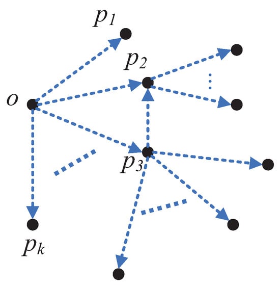
Figure 1.
Illustration of boundary points.
Given a dataset P containing n data points , the Direction Centrality Metric (DCM) is calculated for each data point to evaluate its centrality within the cluster. A smaller DCM value indicates that the data point is closer to the cluster center, while a larger DCM value suggests proximity to the cluster’s edge. For example, as illustrated in Figure 2, DCM can be used to distinguish between interior and boundary points. Data points marked in purple have a relatively uniform distribution of neighboring points, resulting in a smaller variance in the angles between neighbors and thus a lower DCM value, classifying them as interior points. In contrast, data points marked in green exhibit an uneven distribution of neighboring points skewed toward one side, leading to greater variance in neighboring angles and a higher DCM value, identifying them as boundary points.
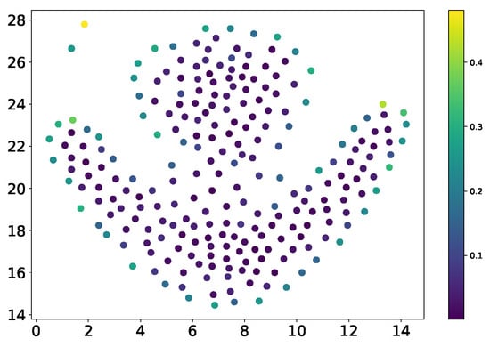
Figure 2.
Scatter plot of weak connectivity.
While the CDC algorithm has demonstrated notable success, it remains challenged by issues in two critical areas, which undermine its effectiveness and efficiency:
- The Challenge In Terms Of Effectiveness: The DCM metric has both advantages and disadvantages. Replacing the density measure with the variance of k-nearest neighbor angles can address the shortcomings of density-based algorithms in identifying sparse clusters. However, this approach may lead to weak connectivity issues, where two high-density regions are mistakenly identified as a single region due to the presence of low-density connecting areas. As illustrated in Figure 3, points of different colors belong to different clusters, the CDC algorithm successfully identifies the green sparse cluster but erroneously merges the red and blue clusters into one. This misclassification occurs because points in sparse regions are recognized as internal points (due to the uniform distribution of k-nearest neighbors and low DCM values). For the green sparse region, this is advantageous, as density-based metrics would fail to identify it as a cluster. However, for the sparse region between the red and blue clusters, the points are incorrectly treated as belonging to a high-density region, resulting in weak connectivity. Developing an effective metric that can both accurately identify sparse clusters and alleviate weak connectivity issues is a challenge that warrants further investigation.
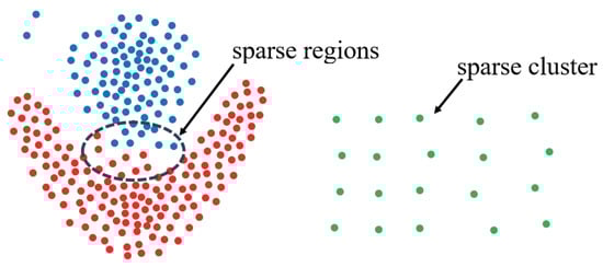 Figure 3. Scatter plot.
 - The Challenge In Terms Of Efficiency: The computational complexity of the CDC algorithm escalates rapidly with increasing data size, primarily due to the intensive distance computations required for determining DCM values. This substantial computational overhead renders the CDC algorithm impractical for efficiently clustering large-scale datasets in a single-machine environment. While distributed computing offers a solution by distributing the workload across multiple servers, most existing methods focus predominantly on partitioning the dataset to minimize the computational and communication costs associated with data replication or repartitioning. Nevertheless, the computational burden within each partition remains prohibitively high, as it necessitates pairwise distance calculations for all points within the group. According to the study [15], the cost of distance computations significantly surpasses that of other tasks, such as data partitioning, in distributed clustering algorithms. Consequently, there is a pressing need for an efficient distributed CDC clustering algorithm that not only ensures the assignment of similar data points to the same partition but also optimizes the computation of DCM values within each partition.
To address the aforementioned challenges, a hybrid metric called “DCM + Density” is proposed to enhance effectiveness. Unlike traditional density-based methods, this metric does not require predefining a neighborhood radius, thereby improving the accuracy of the measurement while reducing its computational cost. For efficiency, a distributed clustering method based on z-value filtering is introduced, reducing the time complexity from to . Our major contributions in this paper are summarized as follows:
- We propose the “DCM + Density” Hybrid Metric. To accurately distinguish boundary points from core points, a hybrid metric is developed by integrating the sparsity indicator () of the region containing a data point with the cluster centralization metric (DCM) employed in the CDC algorithm. Unlike conventional density calculation methods, the computation of does not require a predefined neighborhood radius. Instead, it leverages k-nearest neighbor information obtained during the DCM computation, thus reducing computational overhead. This approach not only preserves the capability to identify sparse clusters but also mitigates issues related to weak connectivity, thereby enhancing the effectiveness of clustering algorithms.
- We develop a distributed direction centrality clustering algorithm enhanced by z-value indexing. This algorithm employs a z-value sorting strategy to allocate proximate data points to the same processing node while pre-copying other required data points to reduce the communication cost of k-nearest neighbor calculations. Furthermore, a z-value curve-based indexing structure is designed to confine the search space to a linear range containing the query point, significantly narrowing the search scope and improving efficiency. Finally, the clustering process is completed through a “local clustering first, cluster merging later” approach, reducing the time complexity from to .
- We conduct extensive experiments to validate the proposed algorithms’ effectiveness and efficiency. First, experiments on two synthetic datasets and five real-world datasets in a single-node environment demonstrated the validity of the proposed metrics. Efficiency experiments further confirmed that the proposed algorithm substantially reduces computation and improves speed. Additionally, experiments in a distributed environment using five real-world datasets were conducted to compare efficiency and scalability, further verifying the algorithm’s high performance and effectiveness.
The remainder of the paper is organized as follows: Section 2 reviews related research work pertinent to this study. Section 3 presents the design of DEALER (Distributed Clustering with Local Direction Centrality and Density Measure), a distributed clustering algorithm enhanced with z-value indexing. Section 5 analyzes the proposed distributed clustering algorithm through experimental testing and evaluation. Section 6 summarizes the work of the full text.
2. Preliminaries
This chapter introduces the clustering method based on Measuring Local Direction Centrality [14] and the related concept of the z-value filling curve.
2.1. Fundamental Concepts
As illustrated in Figure 4, the Direction Centrality Metric (DCM) measures the variance of angles between a given point and its k-nearest neighbors, referred to as the direction centrality of that point. The formal definition of DCM is provided in Equation (1):
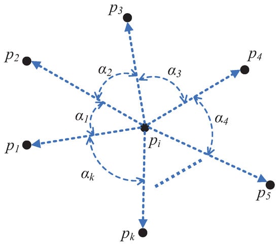
Figure 4.
The Illustration of DCM value calculation.
Definition 1.
Suppose the k-nearest neighbors of a data point are denoted as , arranged in a clockwise order. The DCM value, which quantifies the centrality of , is calculated using the following formula:
The angle is defined as the angle formed at the vertex of the data point between the edge connecting to the j-th neighbor and the edge connecting to the subsequent neighbor in the clockwise direction.
According to the DCM metric, data points can be classified as either boundary points or interior points.
Definition 2
(Interior Points and Boundary Points). Given a DCM threshold and any point p in the dataset P, if the DDCM value of p, denoted as , satisfies , then p is classified as a boundary point. Conversely, if , p is classified as an interior point.
Based on these definitions of interior and boundary points, a cluster can be intuitively understood as a group of interior points that are separated from other clusters by boundary points and other interior points.
2.2. Z-Value Filling Curve
The z-value filling curve maps the coordinates of multidimensional data points into a one-dimensional space, thereby reducing data dimensionality. Figure 5 provides an illustration of the z-value filling curve in a two-dimensional space. The process of z-value transformation is as follows:
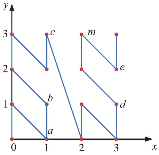
Figure 5.
Illustration of z-value filling curve.
First, the coordinate values of the data points in the high-dimensional space are converted into binary numbers with the same bit length. Then, the binary bits at the same positions across all dimensions are interleaved to form a new binary number. This binary number is subsequently converted into a decimal number, which serves as the z-value coordinate of the data object in the one-dimensional space. Specifically, for a data point p in a d-dimensional space, let its original coordinates be denoted as . Each coordinate value is converted into an mmm-bit binary number. For example, if , the data point is represented in binary form as . The binary sequence is then mapped to a one-dimensional coordinate using Equation (2).
Taking the transformation process of the two-dimensional point d in Figure 5 as an example, first, the coordinate of the data point d in the two-dimensional space is . Next, each dimension’s decimal coordinate is converted into its binary representation. Since , the binary coordinates of point d become . Following this, the coordinate transformation process begins by interleaving the binary bits. The first binary bit from each dimension is extracted, yielding 00. Then, the second binary bit from each dimension is taken, resulting in 10, and so on. Concatenating these bits produces the binary number 001011, which is then converted into its decimal equivalent. Thus, the z-value coordinate of point d on the z-value axis is . This process is illustrated in Figure 6.
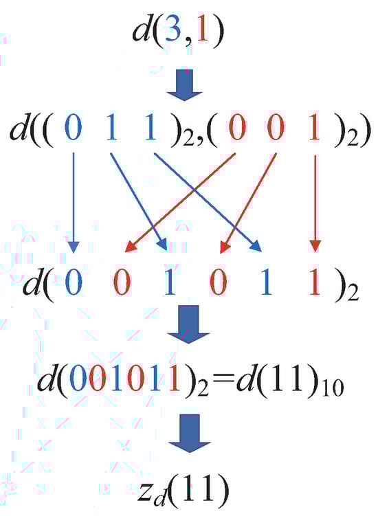
Figure 6.
Illustration of coordinate transformation.
Based on the above coordinate transformation, the six data points in Figure 6 can be mapped into one-dimensional space, as shown in Figure 7.
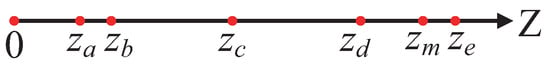
Figure 7.
z-value coordinate representation.
From Figure 5 and Figure 7, the z-value transformation process exhibits the following characteristics. 1. Local Order-Preserving Property: The distribution of data points on the z-value axis roughly preserves the proximity of points in the original space. That is, points that are close to each other in the original space tend to remain close on the z-value axis. 2. Disruptive Changes: In certain cases, the relative distribution of some points may change significantly on the z-value axis. For example, this can be observed in the relationship between points c and m in the figures. The local order-preserving property provides a foundation for using z-values to efficiently identify the range of k-nearest neighbors (KNNs). However, the occurrence of disruptive changes necessitates the design of filtering criteria to ensure the accurate identification of the KNN range.
3. The DEALER Algorithm
This chapter introduces DEALER, a distributed direction centrality clustering algorithm enhanced with z-value indexing. The algorithm refines the DCM (Direction Centrality Metric) by integrating node density information () and leverages distributed computing alongside z-value indexing to accelerate computations. These improvements enhance the CDC (Clustering by Measuring Local Direction Centrality) algorithm in terms of both effectiveness and efficiency.
3.1. Overview
As illustrated in Figure 8, the DEALER algorithm comprises the following steps: (1). Data Partitioning: The data are first sorted based on z-values and divided into tasks, aiming to assign spatially close points to the same partition whenever possible. Additionally, precise quantile-based partitioning is employed to ensure load balancing among subnodes, thereby completing the overall data partitioning process. To facilitate the accurate identification of local K-nearest neighbor (KNN) points in later steps, data replication and range reduction are performed in advance. (2). Computation of DCM and for local clustering: Within each node, local clustering is conducted using two key metrics: DCM, which quantifies the centralization of data points, and , which represents data point density. These measures are combined to distinguish between boundary points and cluster centers. (3). Data Clustering: First, local clustering is performed within each node based on the previously computed directional centrality and density. Then, the initial clusters formed through local clustering are merged to ensure that clusters that should belong to the same group are unified, ultimately achieving the final global clustering outcome. The framework follows a natural logical flow, beginning with data partitioning, followed by intra-partition DCM and density calculations, and concluding with data clustering. To align the framework with the chapter headings for better readability, both local and global clustering are categorized under data clustering. Additionally, since data partitioning involves certain steps and techniques related to intra-partition DCM and density calculations, presenting the computational aspects first enhances clarity. Placing data partitioning at the beginning would necessitate referencing many computational details within that section, leading to a more cumbersome and lengthy explanation. Thus, for conciseness, the order of presentation has been temporarily adjusted.
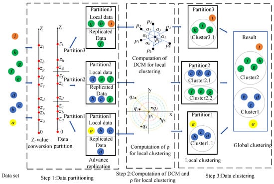
Figure 8.
Overall framework of the algorithm.
3.2. Computation of DCM and for Local Clustering
To facilitate a clearer introduction of the DEALER algorithm, we first present the efficient computation of and DCM values within each partition.
Unlike the CDC algorithm, which relies solely on the DCM metric to distinguish between boundary points and internal points within clusters, the proposed DEALER algorithm incorporates , a metric reflecting the sparsity of the region where a data point resides, into the DCM calculation. As illustrated in Figure 3 in Section 1, this hybrid metric not only maintains the ability to identify sparse clusters but also alleviates issues related to weak connectivity, thereby enhancing the effectiveness of the clustering algorithm. Specifically, the algorithm operates in two steps: First, it computes the DCM value and value for each data point. Using the DCM values, it performs an initial classification, dividing the points into core point candidates and boundary point candidates. Then, the core candidate set is further refined by leveraging the values. Specifically, if a point within the candidate set for internal points has a relatively low value, it is determined not to be an internal point. This screening process is applied to the candidate set, effectively distinguishing internal points from boundary points. Compared to traditional directional-center clustering methods, the incorporation of effectively mitigates weak connectivity issues. Meanwhile, in contrast to conventional density-based clustering, the directional-center assessment based on DCM values demonstrates superior performance in identifying sparse clusters. Under our proposed distributed computing framework, once the data partitioning is complete, the and DCM values for data points within each partition can be computed independently, without requiring inter-node communication.
3.2.1. Computation of DCM
Based on DCM, data points are categorized as either boundary points or internal points. To achieve this, the DCM values for all data points in dataset P must first be computed. The calculation method for DCM values is provided in Equation (1) in Section 2.1. As indicated by the formula, the computation of DCM requires identifying the k-nearest neighbors (KNNs). The primary computational cost of the DEALER algorithm lies in the distance calculations involved in finding KNN points, which represents the bottleneck that constrains the speed of the clustering process. When the dataset size becomes large, the time complexity of for these calculations becomes prohibitively expensive. Thus, improving the algorithm’s speed is essential to meet the demands of large-scale data processing. To accelerate KNN searching, this section proposes a filtering strategy based on a z-value filling curve, referred to as the Z-CF (z-value-based computing filter) algorithm. Before introducing the Z-CF algorithm, we first prove two theorems.
Theorem 1.
In a d-dimensional space, given two data points and , where , , the following holds:
Proof.
For two data points, and , where , , we refer to the method described in Lemma 4 of reference [14], which rearranges the coordinate values by alternating between the most significant bit and the least significant bit to derive the z-value of a point. This implies that . □
Theorem 2.
Given two data points p and q in a d-dimensional space, if the distance between them , then the following holds:
Here, and are new data points derived by subtracting and adding s to each coordinate value of the data point p, respectively. That is, and .
Proof.
If , then for , it holds that . Based on Theorem 1, we can conclude that . □
Since data points, when mapped from high-dimensional space to one-dimensional space via the z-value filling curve, cannot be guaranteed to be ordered strictly by distance, it is necessary to first identify the potential range for the KNN points, then compute the distances within that range and sort the points to obtain the exact KNN. Building on the two theorems mentioned above, after arranging the data points in ascending order based on their z-values, we can efficiently identify the KNN points for any given data point p. This is achieved by iteratively searching in both forward and backward directions along the z-value axis, selecting the closer of the two candidate points at each step. After k iterations, we obtain a point , and it follows that the distance is necessarily greater than the farthest distance among p’s true KNN points. According to Theorem 2, the positions of p’s KNN points along the z-value axis fall within a specific range. Furthermore, Theorem 2 establishes that p’s KNN points must lie within a neighborhood centered at p with a radius of after k comparisons. Within this defined range, an exact KNN search can then be conducted. Compared to traditional KNN searches, incorporating the z-value index significantly reduces the search space by narrowing the potential candidate set from the entire dataset to a localized subset. This approach substantially decreases the number of distance computations required, thereby improving computational efficiency. The detailed strategy and analysis are presented as follows.
First, identify the initial potential KNN points. For a given d-dimensional dataset P, all data points in the dataset are mapped into one-dimensional space via the z-value filling curve so that the z-value coordinates correspond one-to-one with the original space coordinates. Next, the data points are sorted by their z-values. On the z-value axis, the initial potential KNN points are identified. For any data point p, search for one point in each direction along the z-value axis: one in the positive direction, denoted , and one in the negative direction, denoted . The distances between p and these two points, and , are calculated. The point with the smaller distance is selected as the first initial KNN point. Then, along the direction of the closer point on the z-value axis, search for the second point, calculate the distance, and compare it with the previously identified farther point. The point with the smaller distance is selected as the second initial KNN point, and this process continues until k points are identified.
Next, determine the potential range for the KNN points. For any given data point p, the initially identified KNN points are sorted in ascending order of distance. The point that is the k-th closest, denoted as , is selected. The potential range for the KNN points is defined as a neighborhood centered at p with a radius of .
As illustrated in Figure 9, instead of performing a search over the entire data space, a one-dimensional linear search within the interval is sufficient to identify the KNN points of data point p. This is because, for any data point q such that , according to Theorem 2, the z-value of q must lie within the interval . Therefore, there is no need to compute the distances from q to p for the ranges where or , as it is guaranteed that will be greater than .
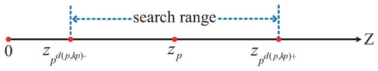
Figure 9.
The illustration of the linear search range.
It is important to note that if, for data points p and q, the lies within the interval , and the lies within the interval , then when calculating the KNN for data point p, the distance needs to be calculated once. Similarly, when calculating the KNN for data point q, the distance must also be calculated once. This results in redundant distance calculations and increases unnecessary computational overhead, as illustrated in Figure 10.
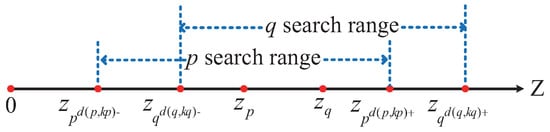
Figure 10.
Illustration of repeated calculations.
To optimize the computational strategy and reduce unnecessary overhead, this study adopts a one-sided computation approach. Specifically, for a given data point p, we calculate the distance only to the points on one side of the interval. This means either computing the distance to the data points in the right-hand interval or to those in the left-hand interval . Both methods yield the same result, and in this paper, the first method is employed, as shown in Figure 11.
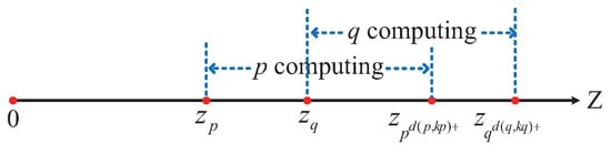
Figure 11.
Illustration of the distance calculation range.
The proposed strategy is based on Theorem 3.
Theorem 3.
Given a dataset P and any data point p, suppose there exists a subset such that for , . The subset is then divided into two subsets, denoted as and , where . For , , and for , . Then, we have the following:
Proof.
Based on Theorem 3, when calculating the distance between data point p and data point q, if , we can compute the distance from p to . Similarly, when calculating the distance from p to with respect to their previous data points in the interval , we can compute the distance from p to all . This reduces the computational load, making the Z-CF algorithm more efficient.
The Z-CF algorithm uses the z-value filling curve to map points from high-dimensional space into one-dimensional space. The z-value filling curve ensures that points that are close in the original space remain close in the one-dimensional space, thereby narrowing the KNN search range. To further reduce redundant calculations, a one-sided calculation strategy is employed to optimize the algorithm. The specific computational process of the Z-CF algorithm is described in Algorithm 1.
| Algorithm 1 Z-CF |
| Input: Dataset P, KNN value k |
| Output: KNN sets and distances for all points in P |
| 1: Transform all data points into one-dimensional space using Equation (2) to obtain |
| 2: Sort the data points by their z-values in ascending order |
| 3: |
| 4: for each data point in do // Find the initial KNN points |
| 5: // Q represents the subset of P with removable points |
| 6: |
| 7: while do |
| 8: , |
| 9: |
| 10: |
| 11: |
| 12: |
| 13: end while |
| 14: Sort by increasing distance in |
| 15: |
| 16: end for |
| 17: for each data point in do |
| 18: Compute and |
| 19: for such that do |
| 20: if then |
| 21: |
| 22: Update |
| 23: end if |
| 24: if then |
| 25: |
| 26: Update |
| 27: end if |
| 28: end for |
| 29: end for |
3.2.2. Computation of
Although clustering methods based on DCM values ensure the identification of sparse clusters, they perform poorly in addressing weak connectivity issues. To maintain the capability of identifying sparse clusters while mitigating weak connectivity problems, a hybrid metric incorporating the -value is introduced. Unlike traditional density computation methods, the calculation of the -value in the DEALER algorithm does not require specifying a neighborhood radius. Instead, it directly uses the reciprocal of the Euclidean distance between a data point and its k-th nearest neighbor, as determined during the DCM computation process, to represent the data point’s density. This approach offers two key advantages. First, it does not introduce additional computational overhead, as it merely applies a reciprocal operation to pre-computed data. Second, the reciprocal of the distance to the k-th nearest neighbor is positively correlated with the density as traditionally defined: the greater the distance to the k-th neighbor, the smaller the reciprocal, indicating sparser surrounding points and lower density in sparse regions, and vice versa. Moreover, using the reciprocal of the distance to the k-th nearest neighbor as a density metric inherently normalizes the density, which facilitates subsequent data processing tasks, such as data filtering. The formal definition of density is provided as follows:
Definition 3
(K-Nearest Neighbor Limited Density). For any data point , if denotes the k-th nearest neighbor of in the data space, then the reciprocal of the Euclidean distance between and is defined as the k-nearest neighbor limited density of the data point .
Figure 12 illustrates the density computation process. As shown, for a given data point , assuming , five nearest neighbors can be identified, denoted as , and sorted by distance in ascending order as . Based on Figure 12, the formula for calculating the density of is presented in Equation (7):
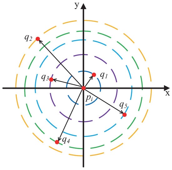
Figure 12.
Illustration of density calculation.
Here, represents the density of the data point , is the k-th nearest neighbor of in the data space (corresponding to point in the figure), and denotes the Euclidean distance between and .
Based on the above analysis, to accurately differentiate between boundary points and core points and further enhance clustering accuracy, it is necessary to classify data objects using a combination of two metrics: density () and local DCM. Within the same cluster, boundary points generally have lower density compared to core points, while their DCM values are higher. Since the core points uniquely determine a cluster, it is essential to ensure all core points are correctly identified. To achieve this, a two-step strategy is employed: first, data objects are filtered based on their DCM values, followed by a secondary filtering based on density values. Specifically, data objects in the dataset are divided into two subsets based on their DCM values: a core point candidate set and a boundary point candidate set. Next, density values are applied to further filter the objects in the core point candidate set. If the density of a data object is smaller than the densities of more than half of its k-nearest neighbors (KNNs), the object is reclassified as a boundary point. This approach is justified because, for objects in the core point candidate set, their KNN points are relatively evenly distributed. If the density of a data object is exceeded by a certain proportion (, typically set to 50%) of its KNN points, the object is likely closer to the cluster boundary. Consequently, the center of the cluster to which this object belongs is biased toward the region with higher-density data points. This methodology provides a clear distinction between core points and boundary points within the dataset, laying a solid foundation for subsequent clustering operations.
3.3. Data Partitioning
This section presents a data partitioning method enhanced by z-value indexing. While addressing the challenge of partitioning data and computational tasks to ensure load balancing, it also requires copying certain data and adjusting data partitions in order to maintain the accuracy of the clustering results.
3.3.1. Initial Data Partitioning
This section introduces the initial data partitioning approach based on z-value indexing. Due to the local ordering property of z-values, points that are close in the original dataset are likely to have similar z-values. To facilitate explanation, two key concepts are introduced: local data and replicated data. As their names suggest, local data are the data inherently residing on a given node, while replicated data are data that do not originally belong to the node but are copied from other nodes due to computational requirements. These concepts are formally defined as follows:
Definition 4
(Local Data). For any sub-node , local data are the data points on which KNN computations are performed locally on the node.
Definition 5
(Replicated Data). For any sub-node , replicated data are data points that do not originally belong to the node but are copied from other nodes to enable the computation of KNN for the local data.
To partition nearby data points into the same sub-node, the distributed clustering algorithm partitions the data based on the z-value information of the data objects in the dataset. The z-value contains the spatial location information of the corresponding data points, meaning that data points that are close to each other on the one-dimensional z-value axis will also be close in the original space. Furthermore, according to the DEALER algorithm, the KNN of a data point is computed using a z-value optimization method. By leveraging this property, data can be partitioned without recalculating the z-values for each data point, ensuring that points that are close in the original space are grouped into the same partition, i.e., the same sub-node. Specifically, for a given dataset P, all data points are first mapped to a one-dimensional space based on the z-value transformation formula (Equation (2)), resulting in a corresponding z-value for each point.
Next, it is necessary to partition all data points in the dataset into distinct subsets to facilitate further processing on different sub-nodes. Specifically, given a dataset P, the data are divided into n equal parts. This is achieved by first calculating the quantile points and then partitioning the dataset into subsets . A sampling-based method introduced in [16] provides a straightforward approach to approximate these quantile points by sampling the data. However, this method often leads to imbalanced load distribution due to inaccuracies in the approximate quantiles. To address this issue, a sorting-based local data partitioning strategy is proposed.
Since the computation of KNN points for local data on each sub-node requires sorting the data based on z-values, the proposed local partitioning strategy performs a global sorting of all data points in the dataset by their z-values. The dataset is then evenly divided into partitions, as illustrated in Figure 13.
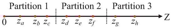
Figure 13.
The illustration of the global sorting partition strategy.
From Figure 13, it can be observed that after sorting the dataset based on the z-values, precise quantile points, such as , can be easily identified. Subsequently, the entire dataset P can be uniformly partitioned into n regions either by redistributing the dataset or by utilizing the precise quantile points. Compared to sampling-based partitioning strategies, this approach introduces additional overhead due to global sorting. However, it ensures the identification of accurate quantile points, thereby achieving load balancing across the sub-nodes. In practice, global sorting is not necessarily an extra expense, as the sub-nodes must locally sort their data based on z-values during their KNN computations. Thus, this strategy provides a balanced trade-off compared to the approximate partitioning strategy based on sampling. Furthermore, due to the properties of z-values, points that are spatially close are often assigned to the same sub-node, which facilitates subsequent local KNN computations.
3.3.2. Data Partition Adjustment
Calculating the exact KNN points on a sub-node is a necessary condition for ensuring the accuracy of DCM and , as well as for ensuring the effectiveness of the clustering results. However, due to the discontinuity of the z-value curve, the global KNN points for a local data point may not all be assigned to the sub-node containing . Therefore, it is necessary to pre-copy the information of all potential KNN points that are not stored locally from other sub-nodes. Once the data copying is completed, each sub-node only needs to compute the KNN values for its local data. Figure 14 illustrates the process of copying data points.
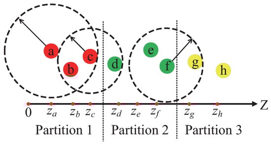
Figure 14.
Illustration of the data copy.
Figure 14 illustrates the process of copying data points. In this figure, assume . In Partition 1, if only local data are considered, the KNN points for data point c would be points a and b, which are clearly inaccurate. To accurately identify the KNN points for c, the position information of point d must be copied from its original sub-node to the sub-node containing Partition 1. In this case, point d becomes a copied data point in Partition 1. Similarly, for data point f, the position information of point g in Partition 3 needs to be copied to Partition 2. By following this process, each sub-node must retrieve partial data from other sub-nodes to ensure the precise computation of KNN points for its local data objects.
The Z-CF algorithm accelerates the clustering process by narrowing the KNN search range through the correspondence between the original space coordinates and the z-values. However, in a fully distributed environment, the true KNN points may reside on other subnodes. Therefore, it is necessary to copy all the data information required to find the local data objects’ exact KNN points from other subnodes. To minimize the communication overhead, the strategy for finding exact KNN points in a distributed environment, called S-KNN (Spark-KNN), is proposed. This strategy is based on the following two theorems:
Theorem 4.
Given a dataset P, , such that , then the following holds:
where is the exact k-th nearest neighbor of data point p, and q is the k-th nearest neighbor found within the same sub-node as p.
Proof.
According to Theorem 2, for , the following holds: and . Since , it follows that , . Therefore, we conclude that . □
Theorem 5.
Given a local dataset on any sub-node, for , if and , the following holds
where q is the k-th nearest neighbor of point p found within sub-node and .
Proof.
Based on the definitions and formulas of and , we know and . Since , and according to Theorem 2, the following holds: . Thus, we can conclude that . □
Based on the theorems above, we propose the S-KNN strategy for accurately finding local KNN points in a distributed environment. First, we discuss how to accurately compute the KNN points for local data on a single sub-node. According to the Z-CF algorithm, for a local data point on a sub-node, the algorithm identifies its k-th nearest neighbor within the sub-node and calculates the distance , which serves as the upper bound for the search range. Next, it computes and and then determines the and z-values for all local data points on the sub-node. Subsequently, all data points with z-values within the interval , but not belonging to the local data, are identified as candidate points for replication. These candidate points are copied to the current sub-node to serve as the dataset for finding accurate KNN points. Finally, the Z-CF algorithm is used to compute the precise KNN points for each local data point on the sub-node. The detailed steps of the S-KNN strategy are provided in Algorithm 2.
| Algorithm 2 S-KNN |
| Input: Dataset P, KNN value k |
| Output: KNN sets and distances for all points in P |
| 1: Transform all data points in dataset P into one-dimensional space using Equation (2), obtaining . |
| 2: Sort the data points by their z-values in ascending order |
| 3: Compute the quantiles and assign data points to corresponding sub-nodes , where . |
| 4: for each sub-node do // Locate initial KNN points |
| 5: for each do |
| 6: Compute and |
| 7: end for |
| 8: |
| 9: |
| 10: Copy all points with z-values in the range to sub-node |
| 11: Use Algorithm 1 to compute the KNN results. |
| 12: end for |
3.4. Data Clustering
This section describes the clustering process from the node to the global level after obtaining directional centrality and density data based on the z-value index.
3.4.1. Local Clustering
Once data points have been labeled as either internal points or boundary points, the clustering problem reduces to clustering internal points and assigning boundary points to clusters. The process begins by clustering nearby internal points into initial clusters, followed by assigning boundary points to their nearest clusters based on distance. The detailed process is as follows.
First, internal points are clustered by expanding outward from a central internal point, forming initial clusters. For this purpose, we propose the Local Expand (LE) algorithm. Before detailing the algorithm, all internal points are initially stored in a separate set . Next, the algorithm selects a random internal point, assigns it a unique and exclusive label and removes it from . Subsequently, it checks whether any of its KNN points are boundary points. If no boundary points are found, all unlabeled KNN points are assigned the same label as the selected data point. If boundary points exist, all unlabeled internal points closer than the boundary points are assigned the same label as the selected data point. These newly labeled points are then removed from , and their KNN points undergo the same process. This continues until no additional points can be labeled, thereby identifying one initial cluster. The process is repeated by selecting another random point from and following the same steps until becomes empty. At this point, all initial clusters are formed. The detailed procedure for the LE algorithm is presented in Algorithm 3.
| Algorithm 3 Local cluster expansion |
| Input: Set of internal points . |
| Output: Initial clusters |
| 1: |
| 2: |
| 3: while do |
| 4: |
| 5: |
| 6: |
| 7: is among the KNN points of , and no KNN points of are boundary points. is unlabeled and its distance to is smaller than the distance between and the nearest boundary point. |
| 8: |
| 9: end while |
Next, the clustering task for boundary points must be completed. Once the initial clusters are established, both the number and shape of the clusters are essentially determined. The clustering of boundary points becomes straightforward: since boundary points are located on the periphery of clusters, they can simply be assigned the same label as the nearest internal point. Specifically, boundary points are stored in a set B. A boundary point is randomly selected, and its KNN points are examined to identify the closest internal point. The boundary point is then assigned the same label as the identified internal point, and the point is removed from B. If all KNN points of the selected boundary point are also boundary points, the nearest boundary point is located, and the same cluster label is applied. If the nearest boundary point itself lacks a cluster label, the nearest boundary point of that point is identified, and the process repeats until all points in B have been labeled.
Through these steps, all data points in dataset P are assigned cluster labels, marking the completion of the clustering algorithm. Points with the same cluster label belong to the same cluster, while points with different labels belong to distinct clusters.
Next, the local clustering strategy LC (Local Clustering) for sub-nodes is introduced. Since each node can compute metrics only for its local data and the copied data contain only information about individual points, local clustering is applied solely to local data. Specifically, each node processes its local data to produce clustering results. This is identical to global clustering in terms of process, as the k-nearest neighbors (KNNs) identified by the S-KNN algorithm are accurate, ensuring precise values for the DCM and metrics. Differentiating between boundary and internal points hinges on the threshold for the DCM metric and the proportion of KNN points with higher density. To facilitate this, the density values () of copied points must be imported from other nodes. Then, using the approach outlined in Section 3.2, the local data are divided into internal and boundary points. Finally, the single-machine local expansion algorithm LE is applied to cluster the local data.
This completes the preliminary clustering process for each sub-node in a distributed environment. Algorithm 4 provides the pseudocode for the local clustering algorithm LC at any given sub-node.
| Algorithm 4 Local clustering |
| Input: Local dataset , copied dataset |
| Output: Initial clusters |
| 1: Utilize Algorithm 2 (S-KNN) to determine the k-nearest neighbors (KNNs) for all points in the local dataset |
| 2: for each do |
| 3: Compute the DCM value of using Equation (1) |
| 4: Compute the density value of using Equation (7) |
| 5: end for |
| 6: for each do |
| 7: Copy the density value to the corresponding node |
| 8: end for |
| 9: Distinguish all as either boundary points or internal points based on the boundary identification method described in Section 3.2 |
| 10: Perform clustering on the local dataset using Algorithm 3 (LE) |
3.4.2. Global Clustering
In the preceding sections, the local clustering of data on individual sub-nodes was completed. However, in the entire data space, data points belonging to the same cluster may have been allocated to different sub-nodes during the data partitioning process. This situation could result in a single cluster being split and clustered into two or more separate clusters by different sub-nodes. To address this issue, this section introduces the concept of global clustering (GC). The goal of global clustering is to merge the initial clusters generated from local clustering, ensuring that data points belonging to the same cluster are correctly grouped together. This strategy ensures that the accuracy of distributed clustering matches or approximates the accuracy of single-machine clustering results. The global clustering strategy is described in detail below.
In distributed clustering, clusters are uniquely determined by their internal points. Thus, the process of cluster merging can be reduced to the merging of internal points. To determine whether two clusters from different sub-nodes need to be merged, the critical condition is whether their internal points share the same label. Specifically, for internal points belonging to two different clusters, if one internal point has no boundary points among its k-nearest neighbors (KNNs), and the other internal point is one of its KNN points, then the two clusters should be merged. Alternatively, if one internal point’s KNN set includes boundary points, but another cluster has an internal point whose distance to the first point is smaller than the distance between the first point and its nearest boundary point, then the two clusters should also be merged. In other words, if clusters belonging to different sub-nodes have internal points that satisfy the conditions for being in the same cluster according to the local clustering algorithm (LE), these clusters are considered part of the same cross-node cluster. Global Clustering Strategy The specific steps of the global clustering strategy are as follows: 1. Save all internal points from the copied dataset into a separate set, . 2. Randomly select an internal point from . This point should retain its original cluster label from its atomic node and ensure the label differs from those on the current sub-node. Remove this point from . 3. Check the KNN set of the selected point in the current sub-node: (1) If no boundary points exist, assign the same cluster label to all KNN points of the selected point. (2) If boundary points exist, assign the same cluster label to all points within a distance smaller than the distance to the nearest boundary point. 4. Update the cluster labels for all points whose internal point labels have changed. Ensure that all points in the same cluster share the same label. 5. Repeat the process by selecting another point from CT and applying the above steps until CT is empty. Through these iterative steps, the merging of clusters is completed. The pseudocode for the global clustering algorithm is presented in Algorithm 5.
| Algorithm 5 Global clustering |
| Input: Initial clusters , sub-nodes |
| Output: Final clusters |
| 1: for each sub-node do |
| 2: Copy the cluster labels of the replicated data points to the sub-node |
| 3: // represents the replicated data points and represents their cluster labels |
| 4: for each do |
| 5: |
| 6: Identify other data points belonging to the same cluster according to the rules in the DEALER algorithm and update their cluster labels |
| 7: end for |
| 8: end for |
Algorithm 6 presents the pseudocode for the DEALER algorithm. The procedure begins with data preprocessing, where the input data are transformed into a one-dimensional z-value coordinate space and sorted (Lines 1–2). The sorted data are then evenly distributed across all worker nodes (Line 3). Each node independently processes its local data partition by computing the required z-value search range for all local data points, leveraging the optimized KNN search method described in Section 3 (Lines 4–7). To ensure all necessary data reside locally, the algorithm proactively replicates remote data falling within the computed range to the respective node (Line 8). The clustering process proceeds in two phases: 1. Local clustering: Each node executes the base clustering algorithm on its local data to generate initial clusters (Line 9). 2. Global cluster merging: The initial clusters from all nodes are aggregated and merged to produce the final global clustering result (Line 10).
| Algorithm 6 DEALER algorithm |
| Input: Data set P, KNN value k, DCM threshold, number of nodes M |
| Output: All clustering in the dataset P: |
| 1: all the data points in the dataset P into one-dimensional space, obtain |
| 2: Sort the number of points according to the value of z from smallest to largest |
| 3: According to the number of nodes, divide the data points on the axis of the z value into M equalilities and assign them to the corresponding node |
| 4: for each data point p in do |
| 5: Compute |
| 6: end for |
| 7: Calculate and |
| 8: Copy data that is not on node in the interval with z values to |
| 9: Execute Algorithm 4 on node to locally cluster to form the initial cluster |
| 10: Run Algorithm 5 to complete the global clustering |
3.5. Time Complexity Analysis
The computational cost of the DEALER algorithm primarily arises from the distance calculations required to identify the k-nearest neighbors (KNNs). This step is also the main bottleneck limiting the speed of the clustering algorithm. Before determining the potential range for KNN, the algorithm uses z-value indexing to map all data points in the dataset onto a one-dimensional coordinate axis and sort them. This step incurs a computational cost of . Next, when calculating the potential range for KNN, the algorithm first identifies the initial KNN points on the z-value coordinate axis. This is performed using a linear search. Since the search requires moving left and right to find k potential KNN points, the algorithm computes the distance between the current data point and other points and performs comparisons. This step has a cost of . Following this, the precise KNN search range is determined based on the relationship between the k-th nearest neighbor and the current data point. This computation incurs an additional cost of . Finally, the algorithm calculates the distance between the current data point and every data point within the determined search range. These data points are those whose z-values fall within the interval , where p is any data point in the dataset, and q is the k-th nearest neighbor of p in the initial KNN set. This step also incurs a cost of . In most cases, , meaning that k is significantly smaller than n. In summary, the overall time complexity of the DEALER algorithm is .
4. Discussion
Our enhancements to the CDC algorithm primarily focus on two key dimensions: clustering effectiveness and computational efficiency.
(1) Effectiveness Enhancement: To improve clustering quality, we developed a hybrid metric integrating DCM with local density (). This integration builds upon CDC’s original DCM cluster centrality metric while incorporating regional density estimation for precise core/boundary point differentiation. The proposed two-step filtering mechanism operates as follows:
Primary screening using DCM values
Secondary refinement through -density evaluation
This dual-filter approach maintains sensitivity for sparse cluster detection while effectively mitigating weak connectivity issues. Unlike conventional density computation requiring predefined neighborhood radii, our method innovatively derives -values directly from k-nearest neighbor (KNN) information generated during DCM calculation. This synergistic reuse of computational byproducts eliminates redundant operations, significantly reducing algorithmic complexity.
(2) Efficiency Optimization: For distributed computing environments, we propose a z-index-enhanced distributed directional centrality clustering algorithm featuring three key innovations: (i) Spatial data organization: z-value ordering optimizes data locality by colocating proximate data points on the same compute nodes with prefetched reference data, minimizing KNN query communication overhead; (ii) Index structure: A novel z-curve-based spatial index constrains KNN searches to linear intervals containing query points, achieving order-of-magnitude search efficiency gains; (iii) Two-phase processing: The “local-clustering-first, global-merging-later” framework reduces overall time complexity from to .
The combined improvements simultaneously enhance both processing capability and clustering accuracy compared to the baseline CDC algorithm, demonstrating superior performance in handling large-scale datasets while maintaining precise cluster separation.
According to the experimental analysis presented below, the algorithm demonstrates strong performance in terms of effectiveness and clustering efficiency. However, the proposed algorithm is not exclusive to CDC, nor is it universally applicable to all clustering methods. Instead, it is particularly suitable for algorithms that rely on neighborhood information for point evaluation, such as certain density-based approaches, where the measurement of points inherently involves their local neighborhoods.
In high-dimensional clustering, the performance of the z-value index is suboptimal. According to the literature [17,18], it is theoretically impossible for a single curve to traverse every point in a given multidimensional discrete space without crossing itself without favoring any particular direction and while completely preserving locality. The topological discontinuities and spatial preservation issues across multidimensional spaces lead to locality loss. Consequently, when dealing with high-dimensional data, the z-value index exhibits poor local order-preserving properties, resulting in increased abrupt changes. Clustering for high-dimensional data remains a key focus for future research.
5. Experiment Analysis
This chapter presents the experimental evaluation of the algorithm proposed in this paper. It compares the algorithm with current mainstream approaches, focusing primarily on the accuracy of the results and the computational time.
5.1. Experimental Setup
The experimental setup section outlines the configuration of the environment required for the experiments and the preparation of datasets. This includes details about the hardware and software environment, dataset preparation, and parameter settings.
5.1.1. Experimental Environment and Datasets
The cluster consists of five servers, each equipped with 24 GB of memory and dual Intel Xeon E5-2420 six-core processors. The servers operate on the Red Hat Enterprise Linux system. Development is conducted using the Eclipse IDE, with Java as the primary programming language.
The experimental datasets selected for this study include both synthetic and real-world datasets: DS1, DS2, Flame, Spiral, Levine, Samusik, UrbanGB, CoverType, Household, Stock, and Sofia. Dataset DS1 consists of 10 spherical clusters, while DS2 contains 6 non-convex clusters with significant density differences. The Flame dataset consists of two clusters, and the Spiral dataset comprises three linear clusters. The Levine dataset, which records human bone marrow cell features, can be obtained from the FlowRepository platform and contains 14 clusters. The Samusik dataset, which records mouse bone marrow cell data, is also available on FlowRepository and includes 24 clusters. The UrbanGB dataset contains geographical coordinates of 469 cities, with 360,177 latitude and longitude points for each city’s districts, counties, towns, and villages. It can be accessed from the UC Irvine repository. The datasets CoverType, Household, Stock, and Sofia do not specify the number of clusters and are primarily used for efficiency analysis. These datasets can be obtained from the UCI Machine Learning Repository and Kaggle platform. The characteristics of these datasets are summarized in Table 1.

Table 1.
Dataset characteristics.
5.1.2. Parameter Settings
In the DEALER clustering algorithm, the key parameters include the k parameter in the “k-nearest neighbors” method and the DCM threshold .
- Parameter k in the “k-nearest neighbors” method: The value of k is set manually based on the characteristics of the dataset and can be estimated according to the dataset size. An empirical function is proposed to express the relationship between k and the dataset size n as follows:Here, represents the smallest integer greater than or equal to n (i.e., the ceiling of n). This function illustrates the increasing trend of k as n grows. However, since the density of points in specific datasets may vary, the fine-tuning of k is performed based on the density of the data in each particular dataset
- DCM Threshold : The DCM threshold is used to distinguish between boundary points and core points. This threshold can be estimated using the method described in the literature [14].
5.2. The Efficiency Analysis
To validate the effectiveness of the DEALER clustering algorithm, this section compares it with four other clustering algorithms on two synthetic datasets (DS1, DS2) and two real-world datasets (Flame, Spiral). The comparison is based on external evaluation metrics, including Clustering Accuracy (ACC) [19], Adjusted Mutual Information (AMI) [20], Adjusted Rand Index (ARI) [21], and F-score [22]. These metrics are used to measure clustering accuracy, providing an overall performance comparison of the clustering results.
(1). Comparison Algorithms: The algorithms compared in this section include the classic k-means clustering algorithm, DBSCAN, DPC, and CDC algorithms. The parameter settings are based on the original configurations provided in the respective algorithmic literature. The specific settings are as follows:
K-means: A classical clustering algorithm that requires the parameter k, which represents the number of clusters.
DBSCAN: A density-based clustering algorithm requiring two parameters—, which defines the radius of the neighborhood, and , which sets the density threshold to distinguish core points from border points.
DPC: A density-peak-based clustering algorithm that requires , the neighborhood radius parameter.
CDC: A clustering algorithm proposed by Gui et al. in 2022 [14], which requires the k-nearest neighbor parameter (k) and an additional parameter for distinguishing core points from border points.
Table 2 presents the parameter settings used for the comparison algorithms on datasets DS1, DS2, Flame, and Spiral, respectively. A dash (“—”) in the tables indicates that the corresponding algorithm does not require that specific parameter.
Table 2.
The clustering-related parameters of various algorithms on the datasets.
(2). Accuracy Comparison: Table 3 presents the performance of the five clustering algorithms across the four evaluation metrics. In each table, the best value for each metric is highlighted in bold.
Table 3.
Clustering metrics of various algorithms on datasets.
The quality of clustering results requires evaluation through specific metrics, which can be divided into internal and external metrics. Internal metrics assess the clustering results without referring to the true data labels, while external metrics compare the predicted labels from the clustering algorithm with the true labels to evaluate clustering quality. Common external metrics include Clustering Accuracy (ACC), Adjusted Mutual Information (AMI), Adjusted Rand Index (ARI), and F-score. This paper primarily uses external metrics to evaluate the clustering algorithms. The ACC metric measures the proportion of data points that are correctly clustered. The ARI metric focuses on pairs of correctly classified data points, rather than individual points, and is an improvement of the Rand Index [23]. NMI, based on information theory, is another clustering evaluation metric. The F-score combines precision and recall into a single measurement. These four metrics are positively correlated with the quality of the experimental results, with higher values indicating better performance.
Table 3 presents the evaluation metrics for clustering quality across four datasets using five different algorithms, with the best values highlighted in bold. It is evident that, regardless of the clustering metric used, the DEALER algorithm consistently achieves the highest number of optimal results. Even in cases where DEALER is not the top performer, its performance is only marginally below the best. In contrast, other algorithms achieve fewer optimal results and occasionally exhibit poor performance on specific datasets due to their underlying clustering principles. Based on the results and analysis, it is clear that DEALER demonstrates excellent clustering performance across various complex datasets, consistently ranking among the top two. Its accuracy is generally above 95%, indicating strong robustness.
5.3. Davies–Bouldin Index and Silhouette Coefficient
This section presents comparative experiments evaluating the DEALER clustering algorithm against four other clustering algorithms on two synthetic datasets (DS1 and DS2) and two real-world datasets (Flame and Spiral). The clustering accuracy is assessed using metrics such as the Davies-Bouldin Index (DB Index) [24] and the Silhouette Coefficient [25]. The Silhouette Coefficient is a widely used metric for evaluating clustering quality, measuring both the cohesion of data points within a cluster and their separation from other clusters. The Davies–Bouldin Index is an internal evaluation metric that assesses clustering performance based on intra-cluster compactness and inter-cluster separation.
(1) Comparison Algorithms: The comparison algorithms used in this section include the classical k-means clustering algorithm, DBSCAN, DPC, and CDC. The parameter settings for these algorithms are based on their original research papers.
(2) Accuracy Comparison: Table k presents the performance of the five algorithms across four evaluation metrics. Among these metrics, the Davies–Bouldin Index has a lower bound of 0, where a smaller value indicates better clustering performance. The Silhouette Coefficient ranges from −1 to 1, where values closer to 1 indicate better clustering quality, meaning that samples are well clustered within their own groups while being well separated from other clusters. However, both metrics are more suitable for convex-shaped clusters and may not be effective for non-convex structures, such as ring-shaped clusters. Additionally, when the dataset contains only a single cluster, both metrics may produce errors and be invalid.
Table 4 presents the clustering quality evaluation metrics for five different algorithms across four datasets. From the data in the table, it is evident that for DS1, where clusters are predominantly convex, most algorithms produce reasonable clustering results. Among them, DEALER demonstrates the best overall performance. However, on the other three datasets, the clustering quality metrics are generally suboptimal. In conjunction with the clustering visualizations shown in Figure 15, Figure 16, Figure 17 and Figure 18, this issue primarily arises because, in these three datasets (excluding DS1), many clusters exhibit non-convex shapes, making these two parameters less suitable and leading to irregular performance. Specifically, in the Flame dataset, weak connectivity causes the CDC algorithm to misclassify the entire dataset as a single cluster. As a result, the Davies–Bouldin Index and Silhouette Coefficient metrics for CDC fail to compute, leading to errors and missing results.
Table 4.
The Davies-Bouldin Index and Silhouette Coefficient of each algorithm on different datasets.
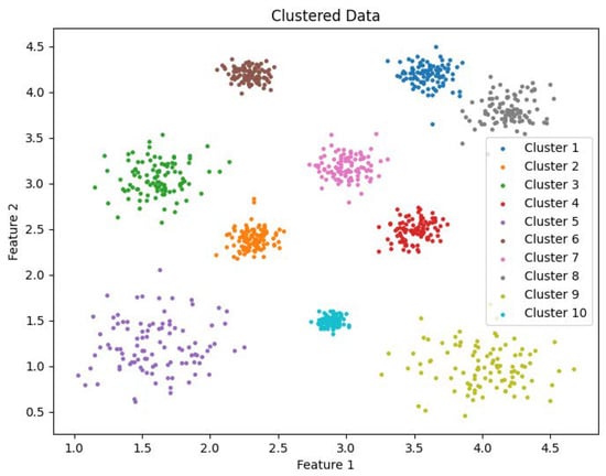
Figure 15.
Clustering visualization: DS1.
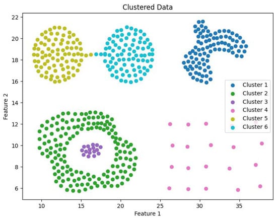
Figure 16.
Clustering visualization: DS2.
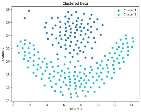
Figure 17.
Clustering visualization: Flame.
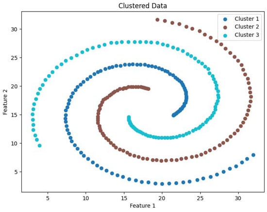
Figure 18.
Clustering visualization: Spiral.
5.4. Impact of Parameter Variations on Clustering Results
This section presents an experimental analysis of the relationship between clustering results and parameter variations in the DEALER algorithm. Specifically, it examines the impact of the number of k-nearest neighbors (k) and the DCM threshold () on clustering performance.
Since the parameters used in this study are similar, the CDC algorithm is selected for comparison with DEALER. However, due to the weak connectivity of the DS2, Flame, and Spiral datasets, the CDC algorithm performs poorly on these datasets. Therefore, the more stable DS1 dataset is used for evaluation, comparing external clustering metrics such as ACC, AMI, ARI, and F-score. Table 5 and Table 6 present the variations in these metrics under different parameter settings. Specifically, Table 5 reports the external metrics when the independent variable is the number of k-nearest neighbors (k), while Table 6 shows the results when the independent variable is the DCM threshold ().
Table 5.
Clustering performance metrics under varying KNN k values when = 0.20.
Table 6.
Clustering performance metrics under varying values when KNN k = 30.
From Table 5 and Table 6, it is evident that DEALER maintains superior clustering performance across a broader range of parameter variations compared to CDC, demonstrating greater stability. The number of k-nearest neighbors (k) has a relatively smaller impact on clustering results over a wide range of values compared to .
5.5. Case Analysis
This section provides a detailed analysis of how the DEALER algorithm ensures the validity of clustering results at each key step. To facilitate a better understanding and visualization of the analysis, we use two datasets, DS1 and Flame, which are easier to visualize. These datasets allow for a more intuitive perception of the data distribution and clustering results. Below, we analyze the parts of the clustering process that directly influence the clustering outcomes.
Based on the analysis in Section 3, it is clear that the resolution of weak connectivity issues depends on the clustering method, especially for datasets with complex structures. Therefore, the choice of clustering method is critical to the clustering results. For better visualization and analysis, we again use the two datasets mentioned above: the synthetic dataset DS1 and the real-world dataset Flame. There are two clustering approaches to compare: one is the method used in the CDC algorithm, which involves surrounding core points with boundary points to form clusters, and the other is the local expansion approach used in DEALER, where clusters are first formed by expanding from center points. Figure 19, Figure 20, Figure 21 and Figure 22 show the scatter plots of the clustering results using the CDC algorithm and the DEALER algorithm, respectively, on the DS1 and Flame datasets.
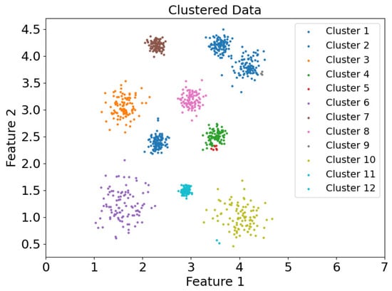
Figure 19.
Scatter plot of clustering results of data et DS1 in the CDC clustering mode.
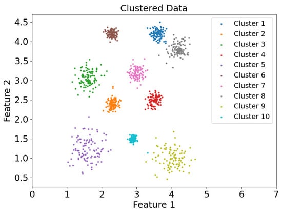
Figure 20.
Scatter plot of clustering results of dataset DS1 in DEALER clustering mode.
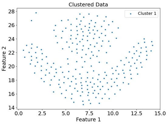
Figure 21.
Scatter plot of clustering results of dataset Flame in CDC clustering mode.
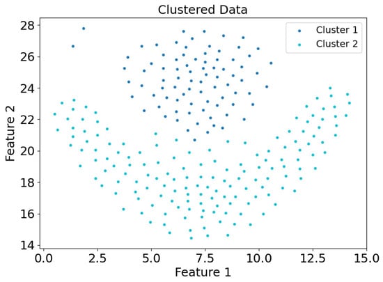
Figure 22.
Scatter plot of clustering results of the dataset Flame in the DEALER clustering mode.
Figure 19 and Figure 20 show the scatter plots of the clustering results for the DS1 dataset using the CDC and DEALER clustering methods, respectively. It is evident that the clustering results obtained with the CDC algorithm are inaccurate. This is because the CDC algorithm uses a boundary-point-enclosing approach for clustering the center points. When the distance between two adjacent boundary points is large, it becomes easy for the algorithm to merge with other clusters that are closer in proximity, leading to the occurrence of weak connectivity issues.
Figure 21 and Figure 22 present the scatter plots of clustering results for the Flame dataset using the CDC and DEALER clustering methods, respectively. It is clear that the DEALER algorithm performs well, producing high-quality clustering results. The local expansion approach used in DEALER allows for clustering by expanding from center points, with expansion halting when a boundary point is encountered. This method effectively mitigates weak connectivity issues to some extent.
Based on the experimental evaluation of the different clustering methods, the accuracy of the clustering results was calculated as follows: On the synthetic dataset DS1, the CDC clustering method achieved an accuracy of 0.7007, while the DEALER method achieved an accuracy of 0.9980, representing an improvement of approximately 42.5%. On the real-world Flame dataset, the CDC clustering method resulted in an accuracy of 0.6375, while the DEALER method achieved an accuracy of 0.9917, representing an improvement of approximately 35.7%. These results demonstrate that the local cluster expansion algorithm outperforms the boundary-point-enclosing center-point algorithm, especially when dealing with complex datasets.
5.6. Efficiency Analysis
In response to the data processing demands of the big data era, distributed clustering algorithms have emerged. This section conducts distributed experiments on the DEALER algorithm to evaluate its efficiency. The dataset used in the experiment has a larger scale. Since no CDC algorithm implementation was found for a distributed environment, comparisons are made between the CDC algorithm, the single-machine version of the DEALER algorithm, and one of the most advanced distributed density-based clustering algorithms, the FDDP algorithm [15]. The experiment is designed with two primary objectives. First, it compares the efficiency of the CDC algorithm, the FDDP algorithm, and the DEALER algorithm in both single-machine and distributed settings. Second, it evaluates the speedup and scalability of the DEALER algorithm.
Figure 23 presents a comparison of the execution time (in seconds) for the CDC algorithm, the FDDP algorithm, and the DEALER algorithm in both single-machine and distributed environments on the given dataset. As shown in Figure 23, the DEALER algorithm demonstrates a higher computational speed compared to the CDC algorithm. Moreover, the distributed implementation of the DEALER algorithm performs well, achieving a slightly better computational speed than the FDDP algorithm.
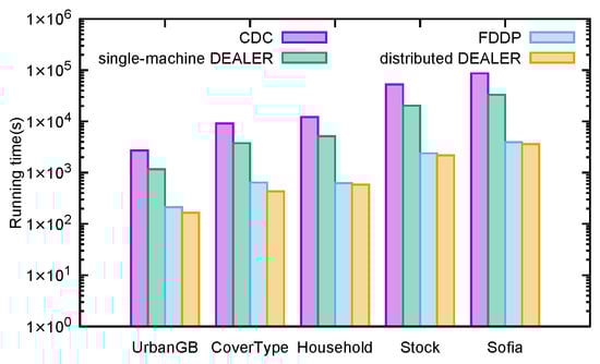
Figure 23.
Runtime of the distributed direction centrality clustering algorithm enhanced by z-value index and existing algorithms.
Figure 24 and Figure 25 present the speedup and scalability performance of the distributed direction centrality clustering algorithm enhanced with z-value indexing. The former shows the proportion of speed improvement in algorithm runtime as the number of distributed system nodes increases, while the latter tests the algorithm’s performance with datasets of increasing size, selected randomly in multiples. The experimental results demonstrate that the z-value-indexing-enhanced distributed-direction centrality-clustering algorithm performs well in terms of both speed and scalability, achieving the expected outcomes of the experiment.
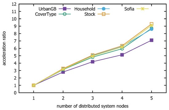
Figure 24.
Distributed algorithm speed ratio.
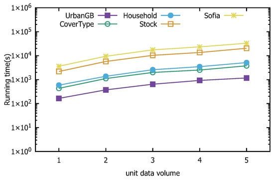
Figure 25.
Distributed algorithm scalability.
5.7. Z-Value Filtering Effectiveness
The improvement in the speed of the clustering algorithm is achieved by optimizing the process of finding k-nearest neighbors using the proposed Z-CF algorithm. This optimization reduces the computational cost of calculating distances between points in the data space, lowering the time complexity from to . The efficiency of the Z-CF algorithm is evaluated through experiments.
In this experiment, seven datasets (ordered by size from smallest to largest: Flame, Spiral, DS2, DS1, Levine, UrbanGB, and Samusik) are used for testing. The objective is to compare the unoptimized k-nearest neighbor search algorithm (KNN-search) with the optimized Z-CF algorithm, which uses z-value filling curves. Table 7 presents the running times (in 10 ms) for computing k-nearest neighbors across different datasets. The variation in running times is ultimately due to differences in the number of computations. Table 8 provides the number of distance calculations performed by each algorithm on the different datasets.
Table 7.
Runtime comparison between the proposed method and baseline approaches.
Table 8.
Distance calculation comparison of the proposed method with baselines.
Based on Table 7, it can be observed that for smaller datasets, the unoptimized KNN-search algorithm performs faster in terms of finding k-nearest neighbors. However, as the dataset size increases, the advantages of the Z-CF algorithm become more apparent, with its efficiency surpassing that of the unoptimized KNN-search. This is because Z-CF reduces the number of distance calculations by narrowing the search range, which in turn decreases computational time. However, since the Z-CF algorithm requires additional computation to determine the new search range, its efficiency is lower for smaller datasets. As the dataset size grows, the efficiency of Z-CF improves, as evidenced by the number of distance calculations presented in Table 8.
To provide a clearer comparison between the two algorithms, the logarithms of the data values are taken, and histograms are shown in Figure 26 and Figure 27. Figure 26 compares the running times across different datasets, while Figure 27 compares the number of distance calculations for each dataset.
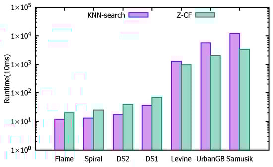
Figure 26.
The running times.
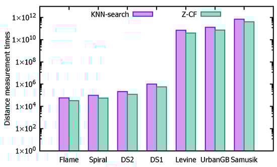
Figure 27.
The number of distance calculations.
6. Conclusions
In this paper, we propose DEALER, an efficient and effective distributed clustering algorithm. Through the proposed density-enhanced local direction centrality measure, DEALER mitigates the weak connectivity problem while maintaining the ability to recognize sparse clusters. Further, the z-value index is designed to reduce the number of distance computations for KNN and enable the communication-free computation of the Direction Centrality Metric DCM and density for the distributed large-scale clustering. We also theoretically prove that DEALER is able to reduce the time complexity of the CDC algorithm from to . A comprehensive experimental evaluation shows that DEALER outperforms the competitors in terms of effectiveness and efficiency and is scalable to large-scale datasets. Facing large-scale data clustering challenges such as those in social networks [26] and genomics [27], the distributed clustering algorithm based on directional centrality discussed in this paper holds significant potential for practical applications. Recent advances have introduced scalable and interpretable clustering frameworks for high-dimensional data [28], including density-based spatial clustering approaches specifically designed for high-dimensional environments [29]. As part of future work, we plan to investigate extensions to the DEALER algorithm that could potentially enhance the performance of these high-dimensional clustering techniques. In the future, we will explore how to extend DEALER to high-dimensional clustering, where the z-value index does not perform very well.
Author Contributions
Conceptualization, Y.Z.; methodology, X.L. and Y.Z.; software, X.L. and Y.Z.; validation, X.L., Z.Z. and Y.Z.; formal analysis, X.L., Z.Z. and Y.Z.; data curation, X.L., Z.Z. and Y.Z.; writing—original draft preparation, X.L.; writing—review and editing, X.L., Z.Z. and Y.Z.; visualization, Y.Z. and X.L. All authors have read and agreed to the published version of the manuscript.
Funding
This work was supported by the National Natural Science Foundation of China (No. 62432003 and 62032013).
Institutional Review Board Statement
Not applicable.
Informed Consent Statement
Not applicable.
Data Availability Statement
The data presented in this study are available on request from the corresponding author.
Acknowledgments
We extend our sincere gratitude to the anonymous reviewers for their valuable insights and feedback.
Conflicts of Interest
The authors declare no conflicts of interest.
References
- Noshari, M.R.; Azgomi, H.; Asghari, A. Efficient clustering in data mining applications based on harmony search and k-medoids. Soft Comput. 2024, 28, 13245–13268. [Google Scholar] [CrossRef]
- Xu, M.; Luo, L.; Lai, H.; Yin, J. Category-Level Contrastive Learning for Unsupervised Hashing in Cross-Modal Retrieval. Data Sci. Eng. 2024, 9, 251–263. [Google Scholar]
- Qu, X.; Wang, Y.; Li, Z.; Gao, J. Graph-Enhanced Prompt Learning for Personalized Review Generation. Data Sci. Eng. 2024, 9, 309–324. [Google Scholar]
- Olszewski, D. A clustering-based adaptive Neighborhood Retrieval Visualizer. Neural Netw. 2021, 140, 247–260. [Google Scholar] [PubMed]
- Djenouri, Y.; Belhadi, A.; Djenouri, D.; Lin, J.C. Cluster-based information retrieval using pattern mining. Appl. Intell. 2021, 51, 1888–1903. [Google Scholar] [CrossRef]
- Paek, J.; Ko, J. K-Means Clustering-Based Data Compression Scheme for Wireless Imaging Sensor Networks. IEEE Syst. J. 2017, 11, 2652–2662. [Google Scholar]
- Anand, S.K.; Kumar, S. Experimental Comparisons of Clustering Approaches for Data Representation. ACM Comput. Surv. 2023, 55, 45:1–45:33. [Google Scholar]
- Martsenyuk, V.P.; Nykytyuk, S.; Palaniza, Y.; Bahrii-Zaiats, O.; Sverstiuk, S. Stages of cluster analysis in the diagnosis of Lyme disease in children. In Proceedings of the ITTAP’2023: 3rd International Workshop on Information Technologies: Theoretical and Applied Problems Ternopil, Ternopil, Ukraine, 22–24 November 2023; pp. 79–92. [Google Scholar]
- Dentamaro, V.; Franchini, F.; Massaro, I.; Musti, L.; Pirlo, G.; Sblendorio, E. Explainable Gait Analysis for Early Detection of Neurodegenerative Diseases Using Unsupervised Clustering Techniques. In Proceedings of the 2024 IEEE International Conference on Metrology for eXtended Reality, Artificial Intelligence and Neural Engineering (MetroXRAINE), St. Albans, UK, 21–23 October 2024; pp. 861–866. [Google Scholar]
- Brotee, S.; Kabir, F.; Razzaque, M.A.; Roy, P.; Mamun-Or-Rashid, M.; Hassan, M.R.; Hassan, M.M. Optimizing UAV-UGV coalition operations: A hybrid clustering and multi-agent reinforcement learning approach for path planning in obstructed environment. Ad Hoc Netw. 2024, 160, 103519. [Google Scholar] [CrossRef]
- Yuan, L.; Xu, Z.; Li, Z.; Zhang, S.; Hu, C.; Yu, W.; Wei, H.; Wang, X.; Geng, Y. Cluster Analysis of Scrna-Seq Data Combining Bioinformatics with Graph Attention Autoencoders and Ensemble Clustering. In Proceedings of the 20th International Conference, Advanced Intelligent Computing in Bioinformatics, Tianjin, China, 5–8 August 2024; Huang, D.S., Pan, Y., Zhang, Q., Eds.; Springer: Singapore, 2024; pp. 62–71. [Google Scholar]
- Zeng, Z.; Zhao, Z.; Xu, K.; Li, Y.; Chen, C.; Zou, X.; Wang, Y.; Wei, W.; Chow, P.K.H.; Li, X. CoIn: Correlation Induced Clustering for Cognition of High Dimensional Bioinformatics Data. IEEE J. Biomed. Health Inform. 2023, 27, 598–607. [Google Scholar]
- Maiti, D.; Basak, M.; Das, D. Advancing Fingerprint Template Generation and Matching With Recast Minutiae Clustering and mRBFN. Adv. Artif. Intell. Mach. Learn. 2024, 4, 1847–1865. [Google Scholar]
- Peng, D.; Gui, Z.; Wang, D.; Ma, Y.; Huang, Z.; Zhou, Y.; Wu, H. Clustering by measuring local direction centrality for data with heterogeneous density and weak connectivity. Nat. Commun. 2022, 13, 5455. [Google Scholar] [PubMed]
- Lu, J.; Zhao, Y.; Tan, K.; Wang, Z. Distributed Density Peaks Clustering Revisited. IEEE Trans. Knowl. Data Eng. 2022, 34, 3714–3726. [Google Scholar]
- Lu, J.; Duan, Y.; Liu, H. Distributed density peaks clustering based on z-value. Acta Electron. Sin. 2018, 46, 730–738. (In Chinese) [Google Scholar]
- Zeng, Q.; Huang, J.; Lu, P.; Xu, G.; Chen, B.; Ling, C.; Wang, B. ZETA: Leveraging Z-order Curves for Efficient Top-k Attention. arXiv 2025, arXiv:2501.14577. [Google Scholar]
- Franco, P.; Mullot, R.; Owczarek, V. Pareto multi-objective optimization for high locality-preserving space-filling curve identification. Swarm Evol. Comput. 2025, 92, 101797. [Google Scholar] [CrossRef]
- Zheng, X.; Cai, D.; He, X.; Ma, W.Y.; Lin, X. Locality preserving clustering for image database. In Proceedings of the 12th Annual ACM International Conference on Multimedia, MULTIMEDIA ’04, New York, NY, USA, 10–16 October 2004; pp. 885–891. [Google Scholar]
- Nguyen, X.V.; Epps, J.; Bailey, J. Information Theoretic Measures for Clusterings Comparison: Variants, Properties, Normalization and Correction for Chance. J. Mach. Learn. Res. 2010, 11, 2837–2854. [Google Scholar]
- Hubert, L.; Arabie, P. Comparing partitions. J. Classif. 1985, 2, 193–218. [Google Scholar] [CrossRef]
- Zhu, Y.; Ting, K.M.; Carman, M.J. Density-ratio based clustering for discovering clusters with varying densities. Pattern Recognit. 2016, 60, 983–997. [Google Scholar]
- Rand, W.M. Objective criteria for the evaluation of clustering methods. J. Am. Stat. Assoc. 1971, 66, 846–850. [Google Scholar] [CrossRef]
- Moulavi, D.; Jaskowiak, P.A.; Campello, R.J.G.B.; Zimek, A.; Sander, J. Density-Based Clustering Validation. In Proceedings of the 2014 SIAM International Conference on Data Mining, Philadelphia, PA, USA, 24–26 April 2014; Zaki, M.J., Obradovic, Z., Tan, P., Banerjee, A., Kamath, C., Parthasarathy, S., Eds.; SIAM: Philadelphia, PA, USA, 2014; pp. 839–847. [Google Scholar] [CrossRef]
- Bagirov, A.M.; Aliguliyev, R.M.; Sultanova, N. Finding compact and well-separated clusters: Clustering using silhouette coefficients. Pattern Recognit. 2023, 135, 109144. [Google Scholar] [CrossRef]
- Meng, L.; Tan, A.; Wunsch, D.C. Adaptive Scaling of Cluster Boundaries for Large-Scale Social Media Data Clustering. IEEE Trans. Neural Netw. Learn. Syst. 2016, 27, 2656–2669. [Google Scholar] [CrossRef] [PubMed]
- Patil, S.; Lora, C.P.; Prabhu, A. Genome Analysis at Scale: Leveraging HPC for AI-Driven Genomics Research. In Proceedings of the 2024 International Conference on Advances in Computing Research on Science Engineering and Technology (ACROSET), Indore, India, 27–28 September 2024; pp. 1–6. [Google Scholar] [CrossRef]
- Belucci, B.; Lounici, K.; Meziani, K. CoHiRF: A Scalable and Interpretable Clustering Framework for High-Dimensional Data. arXiv 2025, arXiv:2502.00380. [Google Scholar]
- Lehner, S.; Enigl, K.; Schlögl, M. Derivation of characteristic physioclimatic regions through density-based spatial clustering of high-dimensional data. Environ. Model. Softw. 2025, 186, 106324. [Google Scholar] [CrossRef]
Disclaimer/Publisher’s Note: The statements, opinions and data contained in all publications are solely those of the individual author(s) and contributor(s) and not of MDPI and/or the editor(s). MDPI and/or the editor(s) disclaim responsibility for any injury to people or property resulting from any ideas, methods, instructions or products referred to in the content. |
© 2025 by the authors. Licensee MDPI, Basel, Switzerland. This article is an open access article distributed under the terms and conditions of the Creative Commons Attribution (CC BY) license (https://creativecommons.org/licenses/by/4.0/).