Optimized Economizer Control with Maximum Limit Set-Point to Enhance Cooling Energy Performance in Korean Climate

Abstract

An air handling unit utilizes economizer control to reduce cooling energy consumption by intaking outdoor air (OA) at lower temperatures. This control modulates OA intake rates based on the OA temperature, adjusting to maximum and partial rates when the OA temperature is below the maximum limit set-point (MLSP), and to minimum rates when it exceeds the MLSP. The MLSP acts as a baseline for determining OA intake rates. However, current MLSPs do not account for the specific OA conditions in South Korea, leading to the intake of unnecessarily warm OA or underutilization of available cooler OA, both of which negatively impact cooling energy performance. Therefore, this study aims to identify the optimal MLSP for OA conditions in South Korea. Through evaluation of cooling energy performance and the indoor thermal environment at various MLSP, it was determined that an MLSP of 22 °C facilitates the lowest cooling energy consumption without adversely affecting the indoor thermal environment. Implementing this MLSP resulted in 5.9% energy savings compared to Case #1 (baseline). The findings indicate that setting an MLSP according to local OA conditions is crucial for maximizing energy savings through economizer control.

1. Introduction

An air handling unit (AHU) utilizes economizer control, which intakes outdoor air (OA) at a lower temperature to reduce cooling energy consumption [1,2]. The economizer control modulates OA intake rates based on the OA temperature. When the OA temperature is below the maximum limit set-point (MLSP), the intake rates are modulated to maximum or partial levels, and the rates are reduced to minimum levels when the OA temperature exceeds the MLSP [3]. Consequently, the economizer control reduces mixed air (MA) temperature by incorporating cooler OA into the AHU, thereby conserving cooling energy [4,5,6].

Economizer control methods are categorized into fixed and differential controls [7]. Fixed control modulates the OA intake rates based on the MLSP, whereas differential control modulates these rates in response to return air (RA) temperature. Differential control, which dynamically modulates the MLSP based on RA temperature, is more effective in saving cooling energy compared to fixed control [8,9]. However, owing to its lower initial costs, simplicity, and ease of maintenance, fixed control is more prevalent in smaller buildings [10,11]. Under fixed control, the OA intake rates are set to maximum and partial levels when the OA temperature is below the MLSP and to minimum levels when it exceeds the MLSP. Thus, the MLSP acts as a baseline for setting OA intake rates [12,13]. Setting the MLSP considerably high can lead to increased cooling energy consumption owing to the intake of unnecessarily warm OA into the AHU (Figure 1). Meanwhile, setting the MLSP considerably low minimizes the potential energy savings from the economizer control, as it fails to intake sufficiently cooler OA. Therefore, it is essential to determine an appropriate MLSP based on the OA conditions, such as dry-bulb temperature and absolute humidity [14,15].

Figure 1. OA intakes by varying MLSP.

To maximize cooling energy savings through economizer control, various studies have been conducted to evaluate the effectiveness of this control by examining OA conditions in different regions. The findings from these studies are summarized as follows:

Chowdhury et al. analyzed the cooling energy consumption of an office building in Australia utilizing economizer control through building energy simulation [16]. Their findings indicated that the total cooling energy consumption and chiller energy consumption decreased by approximately 72 kWh/m²·month and 42 kWh/m²·month, respectively, when economizer control was utilized compared to scenarios without it.

Li et al. evaluated the potential of economizer control in residential buildings across 16 Canadian regions using building energy simulation [17]. The study revealed that, owing to Canada’s mild climate, economizer control could facilitate free cooling for between 50% and 325% of the cooling demand.

Badiei et al. analyzed the cooling energy savings achieved by implementing economizer control in modular data centers located in mild and tropical climates [18]. The results showed significant energy savings of up to 86% in mild climates, while savings in tropical climates were minimal.

Wang and Song studied the effects of economizer control on indoor relative humidity, cooling, and humidifying energy consumption in dry regions using building energy simulations and experiments in an actual building [19]. The results demonstrated that, while maintaining an indoor relative humidity of 30%, cooling energy consumption with economizer control was reduced by approximately 9.3 kW/m³·s compared to cases without economizer control.

Song et al. analyzed the cooling energy consumption of a container farm—a combination of a plant factory and a mobile prefabricated building—across eight regions in China using economizer control [20]. They found that cooling energy consumption was reduced by approximately 58.3% with economizer control compared to the case without it.

Seong and Hong assessed the cooling energy consumption of an educational building employing both fixed and differential economizer control methods using building energy simulation [21]. Their analysis indicated that cooling energy consumption decreased by approximately 49.1% and 49.6% for fixed and differential controls, respectively, compared to the case without economizer control during the interseason.

Choi et al. conducted a study on indoor CO₂ concentration, thermal environment, and cooling energy consumption using fixed and differential controls in an office building modeled using building energy simulation [22]. The analysis maintained indoor CO₂ concentrations for both control methods below the recommended level of 1000 PPM, and indoor temperatures met the cooling set-point. The cooling energy consumption of the differential control method was approximately 4.5 kWh/m² lower than that of the fixed control.

Yao and Wang examined the cooling energy consumption in office buildings utilizing fixed control based on dry-bulb temperature and enthalpy in the northern and southern regions of China [23]. Their analysis revealed that in the hot and humid conditions of the southern region, enthalpy-based fixed control was more effective in conserving energy compared to the dry-bulb-temperature-based control. Conversely, in the low-humidity conditions of the northern region, the dry-bulb-temperature-based control proved more effective.

Lee et al. evaluated the performance of economizer control by adjusting the MA temperature according to OA conditions [24]. They developed a data-driven optimal MA temperature prediction model using MATLAB 2014a and assessed cooling energy performance with TRNSYS. The results indicated an annual cooling energy consumption reduction of approximately 50.4% compared to conventional control methods.

Son and Lee assessed the cooling energy performance using economizer control under varying OA conditions across four regions [25]. An office building was modeled using building energy simulation with weather data from Incheon, Miami, Madison, and San Francisco. The analysis showed that San Francisco, with its lower OA temperature and humidity, achieved the most significant reduction in cooling energy consumption. On the other hand, Incheon, Miami, and Madison, which have higher OA temperatures and humidity, exhibited minimal energy savings.

The studies concerning economizer control methods and MLSP in relation to OA conditions across various regions are summarized in Table 1.

Table 1. Literature review of economizer control.

Ref.	Authors	Location	Building Type	Building Total Floor Area	Economizer Control Method	MLSP
[16]	Chowdhury et al.	Rockhampton, Australia	Office	Medium (4263 m2)	N/A	N/A
[17]	Li et al.	17 regions in Canada 1	Residential	Small (193 m2)	Fixed	N/A
[18]	Badiei et al.	Stockholm, Sweden; Dubai, UAE San Francisco, US; Singapore	Datacenter	Small (12 m2)	Fixed	24 °C
[19]	Wang and Song	Atlanta, US	Commercial	Small (214 m2)	Differential	N/A
[20]	Song et al.	8 regions in China 2	Container farm	Small (15 m2)	Fixed	N/A
[21]	Seong and Hong	Donghae, South Korea	Education	Large (9927 m2)	Fixed and Differential	22 °C
[22]	Choi et al.	Daejeon, South Korea	Office	Large (6164 m2)	Fixed and Differential	24 °C and 28 °C
[23]	Yao and Wang	6 regions in China 3	Office	Medium (4646 m2)	Differential	N/A
[24]	Lee et al.	Ulsan, South Korea	Laboratory	Small (78 m2)	Fixed	18 °C
[25]	Son and Lee	Incheon, South Korea Miami and Madison and San Francisco, US	Office	Medium (1859 m2)	Differential	N/A

¹ Charlottetown, Edmonton, Kamloops, Lethbridge, Montreal, Ottawa, Port Hardy, Prince George, Regina, Sandspit, Saskatoon, Summerland, Toronto, Vancouver, Victoria, Winnipeg. ² Beijing, Guangzhou, Haikou, Harbin, Lanzhou, Mihe, Shanghai, Urumqi. ³ Beijing, Chengdu, Guangzhou, Shanghai, Shenyang, Xi’an.

Previous studies have primarily focused on economizer control implementation to achieve energy savings. These studies analyzed cooling energy consumption with and without economizers, using various control methods. The following issues from the literature review must be considered:

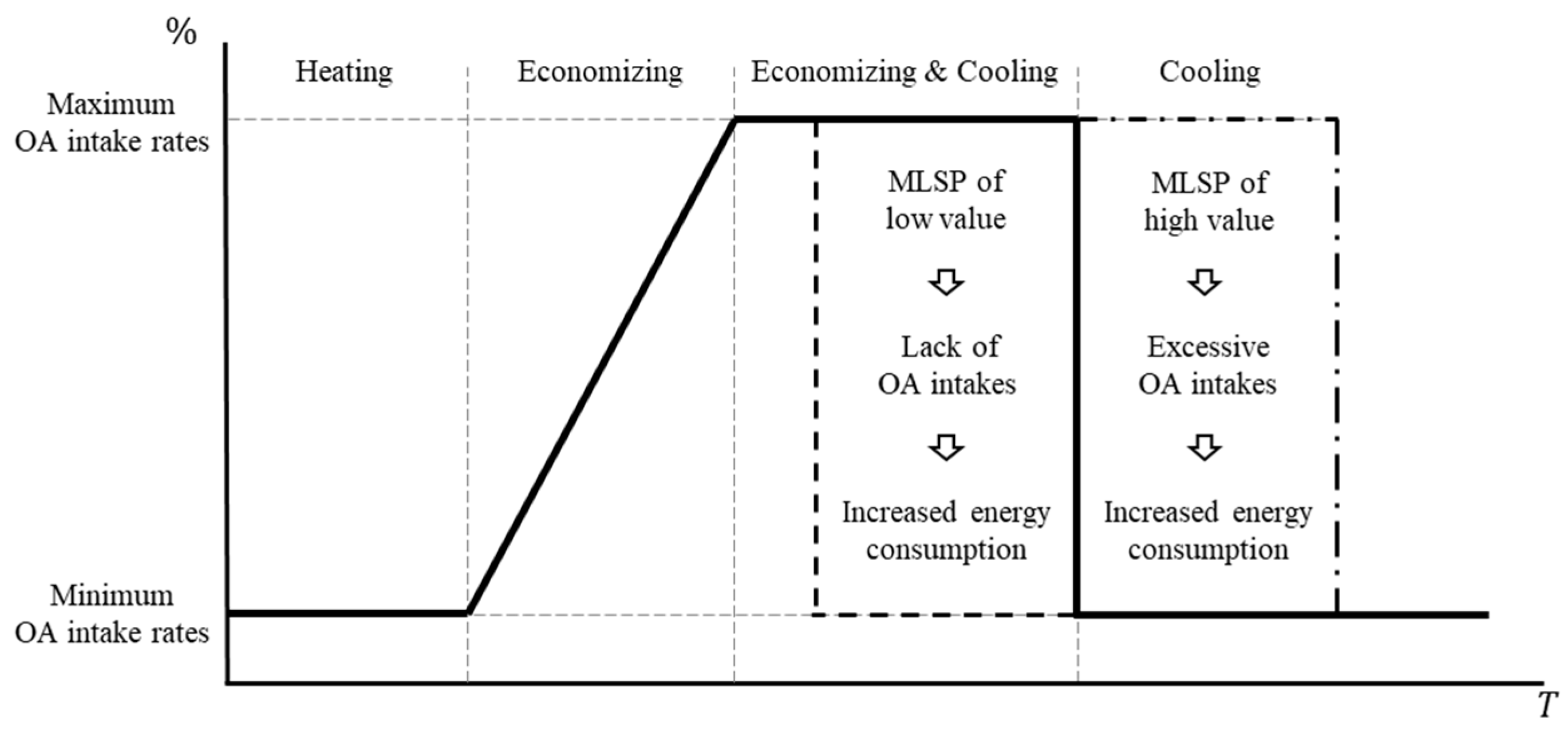
• Economizer control methods: Economizer controls have conventionally utilized fixed control for small buildings and differential control for medium and large buildings.
• Limitations in MLSP determination: Previous research has often overlooked the impact of MLSP on cooling systems. Instead, many studies have utilized the MLSP specified in ASHRAE Standard 90.1 [16,17,18,19,20,23,24,25].
• Limitations in system performance analysis based on MLSP determination: Evaluations of the indoor thermal environment (e.g., dry-bulb temperature and humidity) and cooling energy performance (including OA intakes, air conditions in AHUs, and dehumidification) have not adequately addressed variations in MLSP [21,22].

The MLSP establishes the baseline for determining OA intake rates based on OA conditions. Thus, determining an appropriate MLSP is crucial, taking into account the specific OA conditions. ASHRAE Standard 90.1-2019 specifies MLSP according to OA conditions in the U.S. [26,27]. However, OA conditions in the U.S. differ significantly from those in South Korea, which experiences four distinct seasons with varying humidity levels. Applying the MLSP from ASHRAE Standard 90.1-2019 to economizer controls in South Korea’s cooling systems can lead to increased, unnecessary cooling energy consumption. This increased consumption arises from inappropriate MLSP settings that result in OA intake during suboptimal conditions and rejection during optimal conditions, as well as the intake of high-humidity air, which increases cooling energy consumption owing to the need for dehumidification [28]. Accordingly, determining the MLSP under the Korean climate is necessary to optimize economizer control.

Therefore, this study aims to determine the appropriate MLSP for the Korean climate to achieve cooling energy savings while maintaining an acceptable indoor thermal environment. To achieve this, a parametric analysis was conducted by varying the MLSP to evaluate the indoor thermal environment and cooling energy performance, including OA intakes, air conditions in the AHU, and dehumidification energy consumption.

2. Methodology

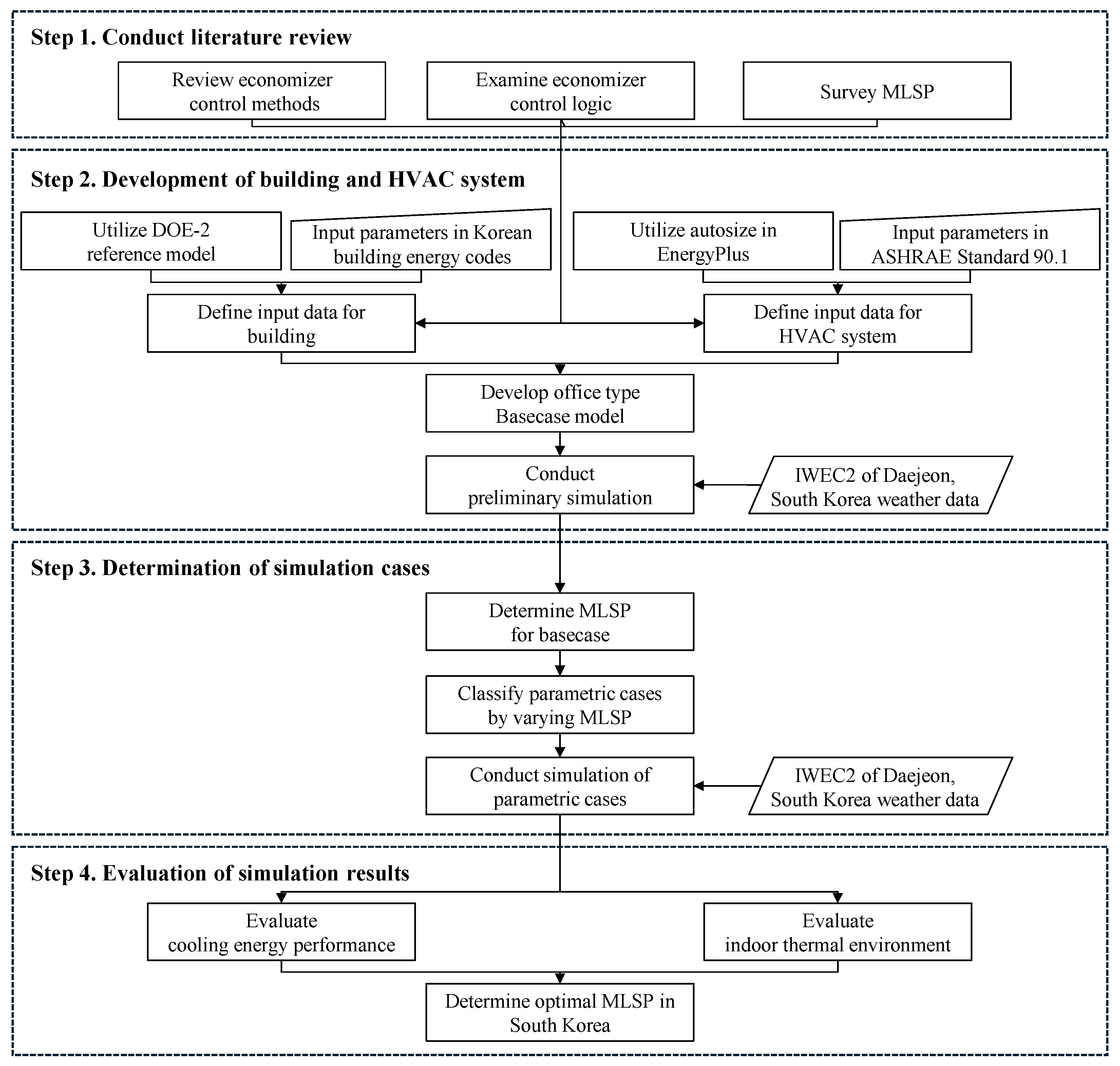
2.1. Overall Study Process

This research was structured into four distinct phases: conducting a literature review, developing building and HVAC (heating, ventilation, and air conditioning) system models, determining simulation cases, and evaluating simulation results. Figure 2 provides a schematic representation of each phase.

Figure 2. Flow chart of overall research methodology.

The initial phase involved a review of the literature on economizer control methods, control logic, and MLSP. During the second phase, a baseline model of an office building and its HVAC system was developed using EnergyPlus Ver. 9.3 [29], a building energy simulation tool. The HVAC system was equipped with economizer control, and preliminary simulations were conducted using this baseline model. In the third phase, parametric cases were classified by varying MLSP, and building energy simulations were conducted for each case. The fourth phase involved the evaluation of cooling energy performance and the indoor thermal environment under different MLSPs. Based on these assessments, the optimal MLSP was determined for South Korea.

2.2. Simulation Modeling

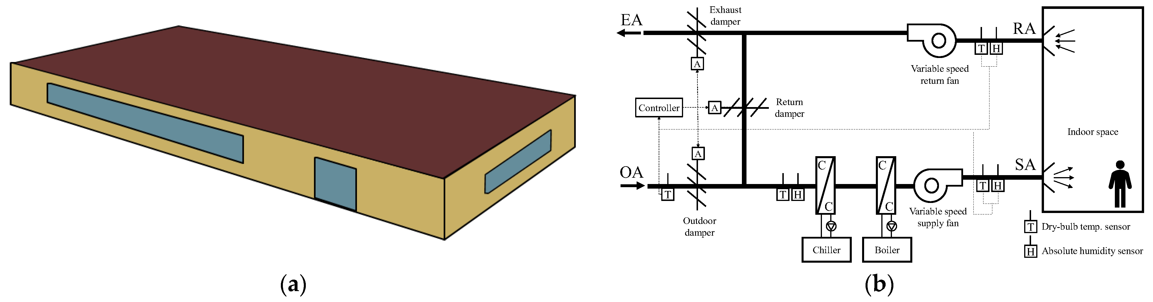
2.2.1. Baseline Model

This study modeled a virtual office building using EnergyPlus Ver 9.3 [29]. Figure 3 shows the building envelope and the schematic of the HVAC system, which was modeled based on the DOE-2 reference model [30]. The building’s volume is 1350 m³ (30 m × 15 m × 3 m). The window-to-wall ratio (WWR) on the north and south sides is approximately 0.4, while on the east and west sides, it is approximately 0.5. Table 2 lists the input values used for the simulation modeling. The indoor cooling set-point was established at 24 °C. Internal heat generation factors from occupants, lighting, and equipment were set at 120 W/person, 6.89 W/m², and 6.78 W/m², respectively, adhering to the guidelines for small offices in ASHRAE Standard 90.1. The HVAC system, a variable-air-volume (VAV) type, controls the air flow to each room. The applied economizer control utilized a fixed method based on dry-bulb temperature [31]. The maximum and minimum OA intake rates were set at 100% and 30%, respectively. The operating hours for the cooling system were scheduled from 7:00 to 18:00 on weekdays as per the Building Energy Efficiency Certification [32]. Cooling system components included an air-cooled chiller, a chilled water coil pump, and a variable-speed fan, with capacities calculated using the autosize function in EnergyPlus, resulting in 19,240 W for the chiller, 292 W for the pump, and 0.4 m³/s for the fan [33]. As the majority of regions in South Korea fall within the 4A climate zone, this study utilized weather data from Daejeon, South Korea, a representative city in this climate classification. Weather data for the simulations were sourced from the international weather files for energy calculation 2.0 (IWEC2) for Daejeon [34]. Economizer control is inactive during winter and summer due to excessively low or high OA temperatures. Therefore, the simulation period was set to the interseason (i.e., Mar., Apr., May, Oct., and Nov.), when economizer control is active. Simulations were conducted at 1 min intervals.

Figure 3. Schematic of simulation baseline model: (a) 3D view of simulation building envelope; (b) simplified simulation HVAC system.

Table 2. Summary of input values used for simulation modeling.

Input Parameters				Values	Information Source
Building	Zone	Use		Office building
		Floor area		450 m2	DOE-2 reference model
		Floor-to-floor height		3 m
		WWR	North and south	0.4
			East and west	0.5
		Indoor cooling set-point		24℃	ASHRAE Standard 90.1-2019
	Heat generation	People		120 W/person
		Light		6.89 W/m2
		Equipment		6.78 W/m2
System	Operation	HVAC		VAV
		Economizer control type		Dry-bulb temperature
		Maximum OA intake rates		100%
		Minimum OA intake rates		30%
		Supply air dry-bulb temperature		13℃	ASHRAE Standard 90.1-2019
		Supply air absolute humidity		0.008 kg/kg’
		Operating hours	Weekdays	07:00–18:00	Building Energy Efficiency Certification
			Weekends	None
	Capacity	Air-cooled chiller		19,240 W
		Cooling water pump		292 W
		Variable-speed fan		0.4 m3/s
Simulation setting		Weather data		Daejeon, South Korea	IWEC2
		Run period		Interseason
		Time-step		1 min

2.2.2. Determination of Simulation Cases

This study identified seven simulation cases by varying the MLSP to evaluate the cooling energy performance and indoor thermal environment. Table 3 presents the classification of these seven simulation cases, each defined by a different MLSP. Case #1 was established with an MLSP of 18 °C, adhering to the standard suggested in ASHRAE Standard 90.1-2019. Cases #2 through #7 were designed for parametric analysis, with the MLSP incrementally increased by 1 °C from 19 °C to 24 °C, aligning with the indoor cooling set-point.

Table 3. Simulation cases by varying MLSP.

Simulation Cases	MLSP [°C]	References
Case #1 (basecase)	18	ASHRAE Standard 90.1-2019
Case #2	19	Parametric analysis
Case #3	20
Case #4	21
Case #5	22
Case #6	23
Case #7	24

3. Results and Analysis

This study aimed to evaluate the cooling energy performance and indoor thermal environment by varying the MLSP and to determine the optimal MLSP based on these results. For this detailed evaluation, simulation results from October, the month when the economizer operated most actively, were selected. Additionally, optimal monthly MLSPs for interseason were determined based on energy consumption evaluations.

3.1. Evaluation of Cooling Energy Performance

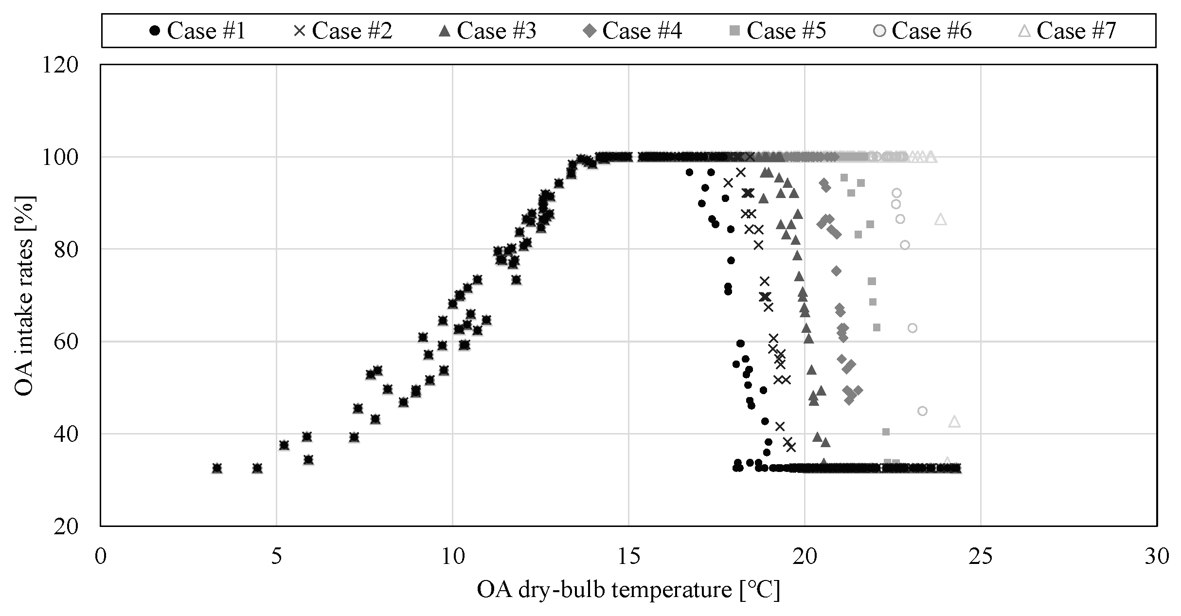
3.1.1. OA Intakes

Section 3.1.1 discusses the evaluation of the OA intakes by varying MLSP. Figure 4 shows the hourly OA intake rates for each case. Table 4 presents the accumulated times for maximum, partial, and minimum OA intake rates, along with the total accumulated OA intakes.

Figure 4. Hourly OA intake rates by varying MLSP.

Table 4. Accumulated times and OA intakes according to OA intake rates.

Simulation Cases	Case #1	Case #2	Case #3	Case #4	Case #5	Case #6	Case #7
Accumulated times of maximum OA intake rates [h]	50	67 (17↑)	83 (33↑)	119 (69↑)	147 (97↑)	165 (115↑)	174 (124↑)
Accumulated times of partial OA intake rates [h]	90	88 (2↓)	87 (3↓)	85 (5↓)	74 (16↓)	68 (22↓)	65 (25↓)
Accumulated times of minimum OA intake rates [h]	102	87 (25↓)	72 (30↓)	38 (64↓)	21 (81↓)	9 (93↓)	3 (99↓)
Accumulated OA intakes [m3/s]	51	56 (5↑)	60 (9↑)	68 (17↑)	73 (22↑)	77 (26↑)	78 (27↑)

The accumulated times for maximum OA intake rates increased progressively from Cases #1 to #7. Meanwhile, the accumulated times for minimum and partial OA intake rates decreased from Cases #1 to #7. This shift occurred because the range of OA temperatures modulated at maximum rates expanded as the MLSP was increased by 1 °C from Cases #1 to #7. The accumulated OA intakes from Cases #2 to #7 increased by increments of 5, 9, 17, 22, 26, and 27 m³/s, respectively, compared to Case #1. This increase was attributed to the reduced frequency of minimum and partial rate periods and the enhanced duration at maximum intake rates. Consequently, as the MLSP was raised, the periods of maximum OA intake rates and, thus, the total accumulated OA intakes increased.

3.1.2. MA Conditions

Section 3.1.2 discusses the evaluation of the MA conditions by varying the MLSP. Figure 5 shows the range of dry-bulb temperature and absolute humidity for the MA. Table 5 presents the average dry-bulb temperature and relative humidity values for analyzing the overall variations in MA conditions by varying MLSP.

Figure 5. MA conditions by varying MLSP: (a) MA dry-bulb temperature; (b) MA absolute humidity.

Table 5. Average MA dry-bulb temperature and absolute humidity by varying MLSP.

Simulation Cases	Case #1	Case #2	Case #3	Case #4	Case #5	Case #6	Case #7
Average MA dry-bulb temperature [°C]	18.13	17.95 (0.18↓)	17.80 (0.33↓)	17.64 (0.49↓)	17.55 (0.58↓)	17.56 (0.57↓)	17.58 (0.55↓)
Average MA absolute humidity [kg/kg’ × 103]	10.12	10.08	9.95	9.77	9.70	9.64	9.63
		(0.04↓)	(0.17↓)	(0.36↓)	(0.43↓)	(0.48↓)	(0.49↓)

The average MA temperature from Cases #2 to #7 decreased progressively compared to Case #1 by approximately 0.18, 0.33, 0.49, 0.58, 0.59, and 0.55 °C, respectively. This reduction was attributed to increased intakes of cooler OA compared to Case #1. Notably, Case #5 exhibited the lowest MA temperature among all cases, resulting from the utilization of maximum OA intakes under favorable conditions, unlike Cases #1 to #4. Cases #6 and #7 utilized maximum OA intakes at temperatures higher than the indoor air. The average MA absolute humidity in Cases #2 to #7 also decreased relative to Case #1, driven by the intake of OA with lower absolute humidity than the indoor air, thus reducing the indoor air absolute humidity as the OA intake increased. Consequently, the reductions in MA temperature across Cases #2 to #7 compared to Case #1 are expected to decrease cooling coil loads and subsequently reduce the cooling energy consumption needed to lower the MA temperature to the supply air set temperature.

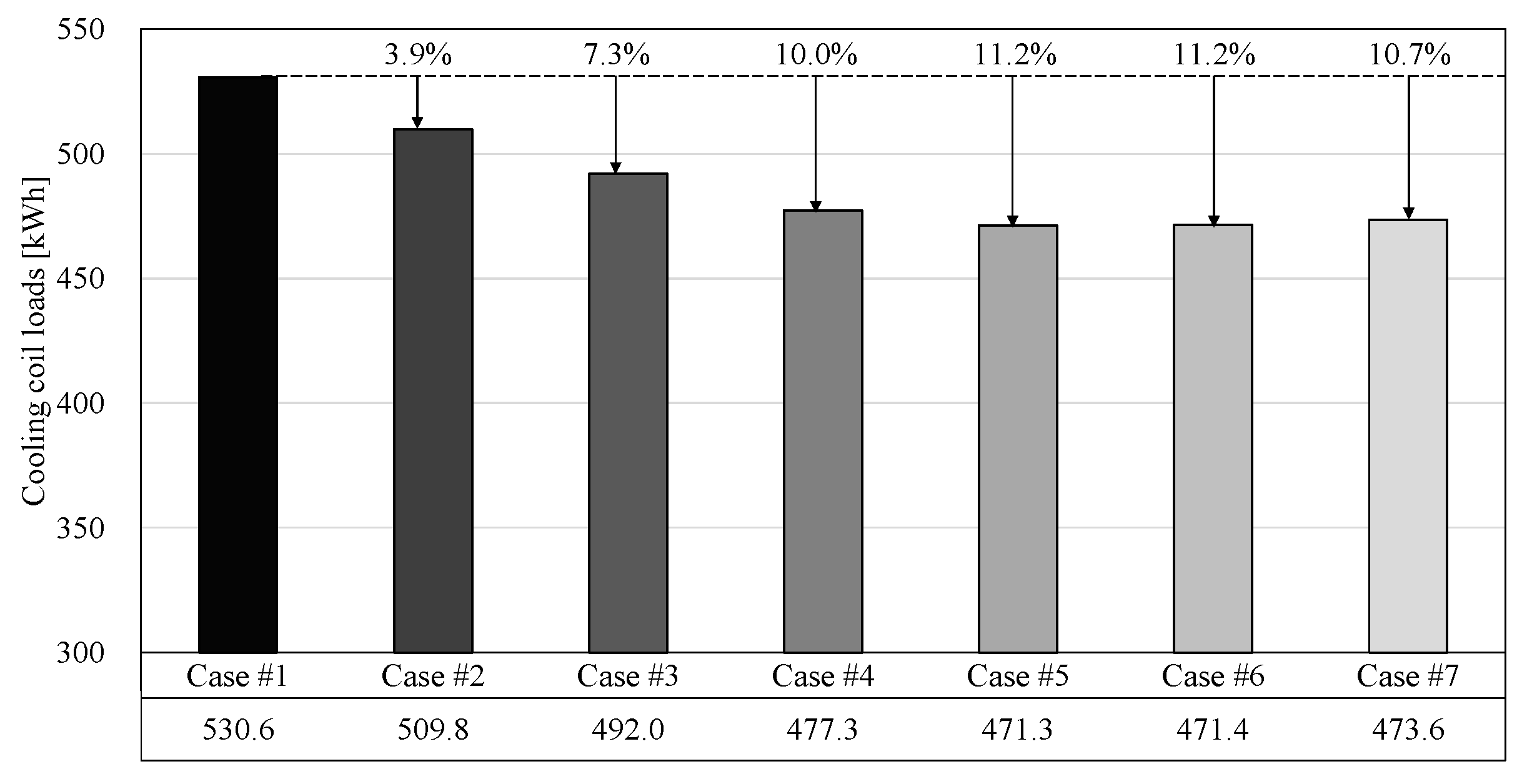
3.1.3. Cooling Coil Loads

Based on the results from Section 3.1.2, the cooling coil loads were anticipated to decrease owing to the reduced MA temperatures. Section 3.1.3 describes the evaluation of the cooling coil loads by varying MLSP. Figure 6 shows the cooling coil loads for each case, calculated using the following equation:

$$q=\rho \times Q\times C_p\times (t_{MA}-t_{SA}),$$

(1)

where $q$ is the cooling coil load, $\rho$ is the air density, $Q$ is the air flow rate, $C_p$ is the specific heat capacity, $t_{MA}$ is the MA temperature, and $t_{SA}$ is the supply air temperature.

Figure 6. Cooling coil loads by varying MLSP.

The cooling coil loads for Cases #2 to #7 decreased by 3.9%, 7.3%, 10.0%, 11.2%, 11.2%, and 10.7%, respectively, compared to Case #1. This reduction was primarily due to the decreased temperature differential between the MA and supply air temperatures. Case #5 exhibited the largest reduction in cooling coil loads, owing to the effective use of maximum OA intakes under available conditions. These results indicate that the cooling coil loads for Cases #2 to #7 were reduced relative to Case #1, driven by the diminished difference between the MA and supply air temperatures.

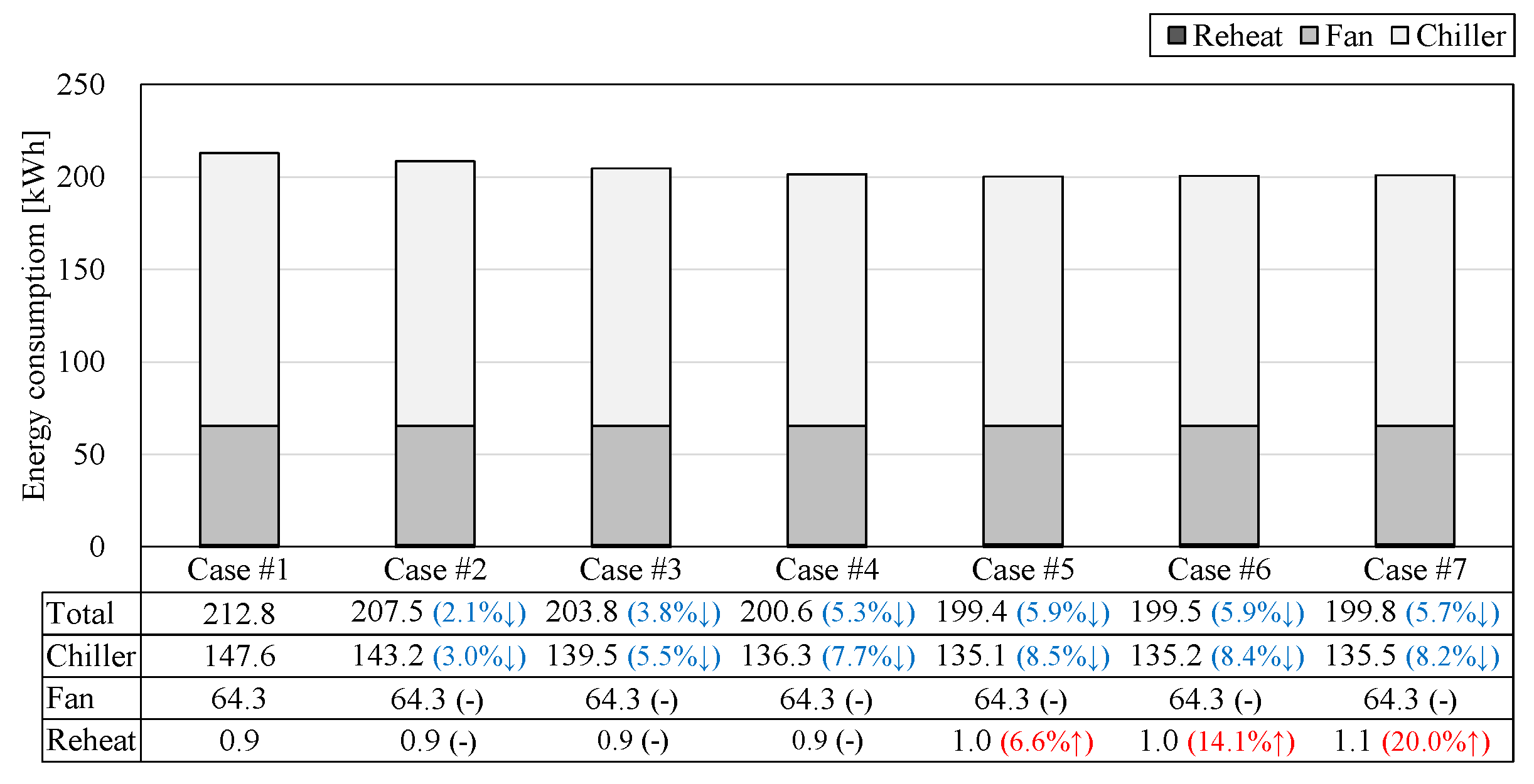
3.1.4. Cooling Energy Consumption

Section 3.1.4 discusses the evaluation of the cooling energy consumption by varying the MLSP. Figure 7 shows the cooling energy consumption for each case, including totals for the chiller, fan, and reheat systems. Chiller energy consumption accounts for the energy used by the chilled water circulation pump. Reheat energy consumption encompasses the energy used by the boiler and hot water circulation pump.

Figure 7. Cooling energy consumption by varying MLSP.

The chiller energy consumption from Cases #2 to #7 decreased by 3.0%, 5.5%, 7.7%, 8.5%, 8.4%, and 8.2%, respectively, compared to Case #1. This reduction was attributed to the decreased cooling coil loads, which, in turn, lowered the chiller loads. Fan energy consumption remained constant across all simulation cases because the supply air reached the set-point temperature in the chiller before reaching the fans, resulting in the fans operating at minimum loads. For reheat energy usage, Cases #2 to #4 showed the same levels, while Cases #5 to #7 exhibited a minor increase compared to Case #1. Consequently, the total cooling energy consumption for Cases #2 to #7 decreased by 2.1%, 3.8%, 5.3%, 5.9%, 5.8%, and 5.7%, respectively, relative to Case #1, primarily due to reductions in chiller energy consumption. Notably, Case #5 demonstrated the greatest savings among all simulation cases. These results suggest that the MLSP recommended by ASHRAE Standard 90.1 may not be optimal for economizer control in South Korea, highlighting the need to establish a region-specific MLSP that aligns with the OA conditions in South Korea.

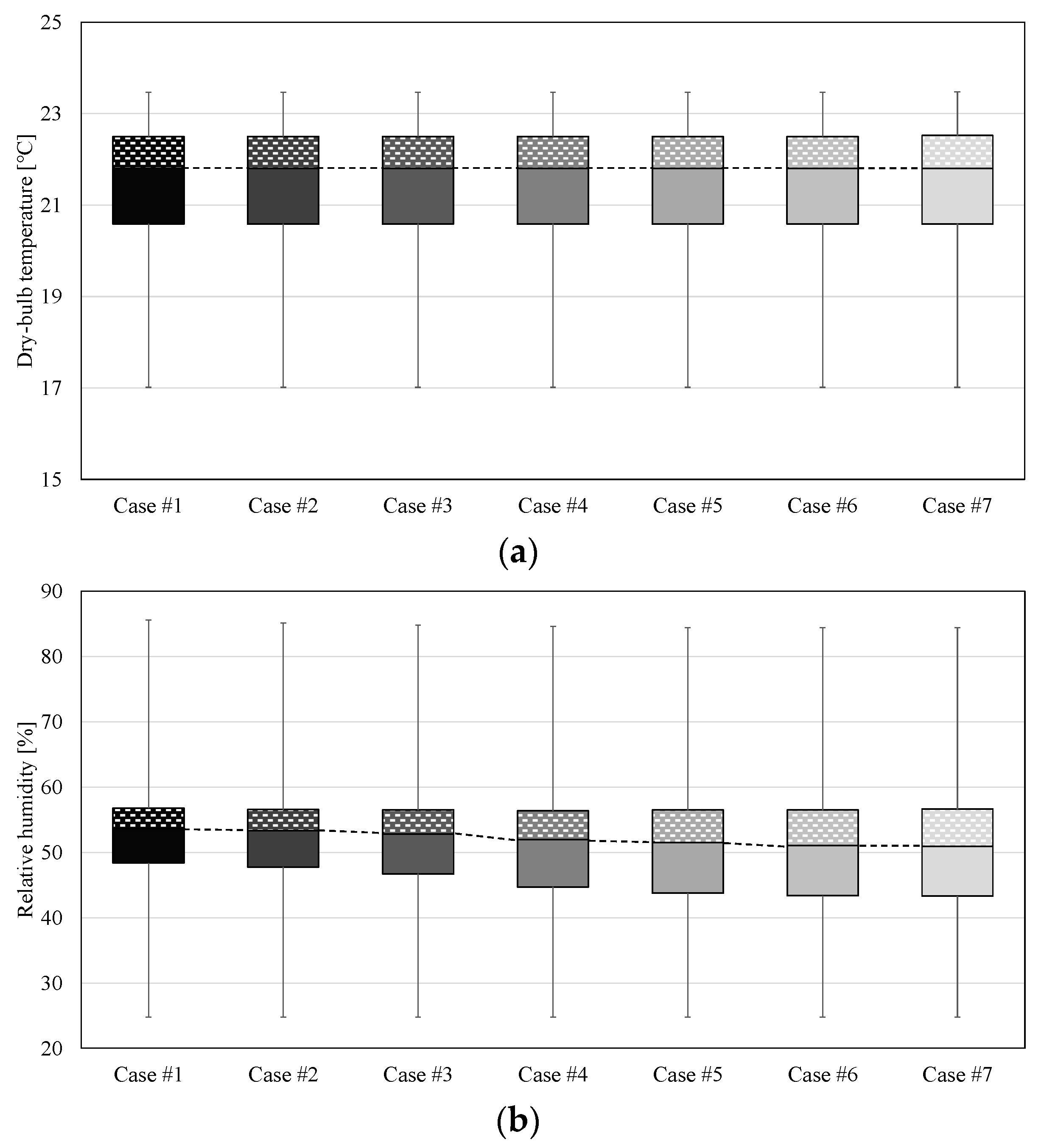
3.2. Evaluation of Indoor Thermal Environment

Section 3.2 evaluates the indoor thermal environment by varying MLSP. Figure 8 shows the indoor air dry-bulb temperature and relative humidity for each case.

Figure 8. Indoor thermal environment by varying MLSP: (a) indoor air dry-bulb temperature; (b) indoor air relative humidity.

In all simulation cases, the indoor air dry-bulb temperature was maintained below the indoor cooling set-point temperature owing to the supply air reaching the set-point in all scenarios. The relative humidity of indoor air decreased progressively from Cases #1 to #7, attributed to the corresponding decrease in MA absolute humidity across these cases. Consequently, as more OA was introduced, the relative humidity of indoor air decreased. This evaluation demonstrated that the indoor thermal environment remained stable despite variations in MLSP. Based on these findings, the optimal MLSP for this evaluation period was determined to be Case #5 (22 °C), which maintained stable indoor thermal conditions while achieving the lowest cooling energy consumption.

3.3. Determination of Optimal MLSP During Interseason

Considering the variability of OA conditions throughout the year in South Korea, this study determined the optimal MLSP for the interseason, excluding October, which served as the primary evaluation period. Figure 9 shows the cooling energy consumption for each month during the interseason. In April and May, Cases #6 and #5 exhibited the lowest cooling energy consumption, respectively. The lowest cooling energy consumption extended from Cases #2 to #7 in March and from Cases #3 to #7 in November. This variation in optimal MLSP each month was due to monthly changes in OA conditions. During this period, the cooling energy consumption was consistent across Cases #2 to #7 in March and across Cases #3 to #7 in November, as the OA temperatures in March and November did not exceed 19 and 20 °C, respectively, resulting in uniform OA intakes. This analysis highlights the importance of defining MLSP according to the specific OA conditions of each month to maximize cooling energy savings through economizer control.

Figure 9. Cooling energy consumption for each month by varying MLSP.

4. Conclusions

This study aimed to determine the appropriate MLSP for OA conditions in South Korea. To achieve this, a base-case model was developed, and building energy simulations were conducted by varying the MLSP. The simulations evaluated cooling energy performance including OA intakes, MA conditions, cooling coil loads, and cooling energy consumption and the indoor thermal environment, notably indoor air dry-bulb temperature and relative humidity. The key findings from this study are summarized as follows:

(1).

Cooling energy performance: Evaluation revealed that Case #5 had the lowest cooling energy consumption among all cases during the primary evaluation period in October. Compared to Case #1 (baseline), which set the MLSP based on ASHRAE Standard 90.1-2019, Case #5 used approximately 5.9% less cooling energy. This indicates that the MLSP of Case #5 provided the most optimal OA intake conditions. The average MA temperature in Case #5 was approximately 0.58 °C lower than that of Case #1. When the MLSP was set for Cases #1 to #4, these did not intake OA under available conditions, whereas Cases #6 and #7 maintained OA intake at conditions where the OA temperature exceeded indoor air temperature. Owing to these differences, Case #5 achieved energy savings compared to the other cases.

(2).

Indoor thermal environment: Evaluation showed that the indoor air dry-bulb temperature was maintained below the cooling set-point temperature in all simulation cases. Additionally, indoor relative humidity exhibited a decreasing trend as OA intakes increased. Therefore, this study suggests that raising the MLSP did not adversely affect the indoor thermal environment.

(3).

Optimal MLSP for interseason: The evaluation of the optimal MLSP for each month in the interseason (March, April, May, and November) indicated that optimal MLSPs were as follows: Cases #2 to #7 in March, Case #6 in April, Case #5 in May, and Cases #3 to #7 in November. This variation was due to monthly changes in OA conditions, necessitating the application of an appropriate MLSP for each month’s specific OA conditions.

These results highlight the importance of defining MLSP according to OA conditions in economizer control. When the optimal MLSP was determined for the South Korean climate conditions (Case #5), cooling energy consumption was reduced by up to 5.9%. Thus, this study contributes to the precise determination of MLSP for economizer control in South Korea’s diverse climate conditions.

However, this study focused exclusively on the MLSP of dry-bulb temperature-based fixed control for economizer control in Daejeon, South Korea. Therefore, future research should address factors such as regional diversity, economizer control methods, and dynamic MLSP control. Additionally, evaluations of cooling energy performance and indoor thermal environment by varying MLSP in this study were based on simulation data. Validation with real buildings will be required in the future to consider the applicability of the optimal MLSP determined in this study to real buildings.

References

- Yoon, Y.; Seo, B.; Cho, S. Potential Cooling Energy Savings of Economizer Control and Artificial-Neural-Network-Based Air-Handling Unit Discharge Air Temperature Control for Commercial Building. Buildings 2023, 13, 1174. [Google Scholar] [CrossRef]
- Dharmasena, P.; Nassif, N. Testing; Validation, and Simulation of a Novel Economizer Damper Control Strategy to Enhance HVAC System Efficiency. Buildings 2024, 14, 2937. [Google Scholar] [CrossRef]
- Kim, C.H.; Lee, S.C.; Park, K.S.; Lee, K.H. Analysis of thermal environment and energy performance by biased economizer outdoor air temperature sensor fault. J. Mech. Sci. Technol. 2022, 36, 2083–2094. [Google Scholar] [CrossRef]
- Lee, K.; Chen, H. Analysis of energy saving potential of air-side free cooling for data centers in worldwide climate zones. Energy Build. 2013, 64, 103–112. [Google Scholar] [CrossRef]
- Ham, S.; Kim, M.; Choi, B.; Jeong, J. Energy saving potential of various air-side economizers in a modular data center. Appl. Energy 2015, 138, 258–275. [Google Scholar] [CrossRef]
- Ghiaus, C.; Allard, F. Potential for free-cooling by ventilation. Solar Energy 2006, 80, 402–413. [Google Scholar] [CrossRef]
- Mu, B.; Li, Y.; House, J.M.; Salsbury, T.I. Experimental evaluation of anti-windup extremum seeking control for airside economizers. Control. Eng. Pract. 2016, 50, 37–47. [Google Scholar] [CrossRef]
- Trane, Airside Economizers and Their Application. 2015. Available online: https://www.trane.com/content/dam/Trane/Commercial/global/products-systems/education-training/engineers-newsletters/airside-design/ADM-APN054-EN_05202015.pdf (accessed on 22 January 2025).
- Hong, G.; Kim, C. Investigation of energy savings potential of multi-variable differential temperature control in economizer. Appl. Therm. Eng. 2021, 197, 117415. [Google Scholar] [CrossRef]
- Seem, J.E.; House, J.M. Development and evaluation of optimization-based air economizer strategies. Appl. Energy 2010, 87, 910–924. [Google Scholar] [CrossRef]
- Wang, S.K. Handbook of Air Conditioning and Refrigeration, 2nd ed.; McGraw-Hill Companies Inc.: New York, NY, USA, 2001. [Google Scholar]
- Kim, M.; Jin, S.; Jang, A.; Park, B.; Do, S.L. Simulated analysis on cooling system performance influenced by faults occurred in enthalpy sensor for economizer control. In Proceedings of the 10th International Conference on Construction Engineering and Project Management (ICCEPM), Sapporo, Japan, 29 July–1 August 2024; pp. 1002–1009. [Google Scholar] [CrossRef]
- Kim, J.H.; Shin, D.U.; Kim, H. Data Center Energy Evaluation Tool Development and Analysis of Power Usage Effectiveness with Different Economizer Types in Various Climate Zones. Buildings 2024, 14, 299. [Google Scholar] [CrossRef]
- Zhou, J.; Wei, G.; Turner, W.D.; Claridge, D.E. Airside economizer—Comparing different control strategies and common misconceptions. In Proceedings of the Sixteenth Symposium on Improving Building Systems in Hot and Humid Climates, Plano, TX, USA, 15–17 December 2008; Texas A&M University: College Station, TX, USA, 2008. Available online: https://hdl.handle.net/1969.1/90706 (accessed on 22 January 2025).
- Taylor, S.T.; Cheng, C.H. Economizer High Limit Controls and Why Enthalpy Economizers Don’t Work. Am. Soc. Heat. Refrig. Air-Cond. Eng. (ASHRAE) 2010, 52, 12–28. [Google Scholar]
- Chowdhury, A.A.; Rasul, M.G.; Khan, M.M.K. Modelling and analysis of air-cooled reciprocating chiller and demand energy savings using passive cooling. Appl. Therm. Eng. 2009, 29, 1825–1830. [Google Scholar] [CrossRef]
- Li, B.; Wild, P.; Rowe, A. Free cooling potential of air economizer in residential houses in Canada. Build. Environ. 2020, 167, 106460. [Google Scholar] [CrossRef]
- Badiei, A.; Jadowski, E.; Sadati, S.; Beizaee, A.; Li, J.; Khajenoori, L.; Nasriani, H.R.; Li, G.; Xiao, X. The energy-saving potential of air-side economisers in modular data centers: Analysis of opportunities and risks in different climates. Sustainability 2023, 15, 10777. [Google Scholar] [CrossRef]
- Wang, G.; Song, L. An energy performance study of several factors in air economizers with low-limit space humidity. Energy Build. 2013, 64, 447–455. [Google Scholar] [CrossRef]
- Song, R.; Liu, D.; Pan, Y.; Cheng, Y.; Meng, C. Container farms: Energy modeling considering crop growth and energy-saving potential in different climates. J. Clean. Prod. 2023, 420, 138353. [Google Scholar] [CrossRef]
- Seong, N.; Hong, G. Evaluation of Operation Performance Depending on the Control Methods and Set Point Variation of the Economizer System. J. Korean Inst. Archit. Sustain. Environ. Build. Syst. 2022, 16, 94–107. [Google Scholar] [CrossRef]
- Choi, B.; Kim, H.; Cho, Y. A study on Performance Evaluation of Economizer Type through Simulation in Office. J. Korean Inst. Archit. Sustain. Environ. Build. Syst. 2015, 9, 229–234. [Google Scholar]
- Yao, Y.; Wang, L. Energy analysis on VAV system with different air-side economizers in China. Energy Build. 2010, 42, 1220–1230. [Google Scholar] [CrossRef]
- Lee, J.; Jo, H.; Cho, Y. Mixed air temperature reset by data-driven model for optimal economizer control. Appl. Therm. Eng. 2024, 238, 122158. [Google Scholar] [CrossRef]
- Son, J.E.; Lee, K.H. Cooling energy performance analysis depending on the economizer cycle control methods in an office building. Energy Build. 2016, 120, 45–57. [Google Scholar] [CrossRef]
- ASHRAE Standard 90.1; Energy Standard for Building Except Low-Rise Residential Buildings. American Society of Heating, Refrigerating and Air-Conditioning Engineers (ASHRAE): Atlanta, GA, USA, 2019.
- Jang, A.; Jin, S.; Kim, M.; Kang, H.; Do, S.L. Evaluation of Cooling Energy Consumption Varying Economizer Control and Heat Generation Rates from IT Equipment in Data Center. In Proceedings of the 10th International Conference on Construction Engineering and Project Management (ICCEPM), Sapporo, Japan, 29 July–1 August 2024; pp. 1010–1017. [Google Scholar] [CrossRef]
- Lee, J.; Cho, Y. Optimal Control of Air-side Economizer. Energies 2024, 17, 5383. [Google Scholar] [CrossRef]
- DOE. EnergyPlus, Version 9.3; Department of Energy (DOE): Washington, DC, USA, 2020.
- DOE. Commercial Reference Building; Department of Energy (DOE): Washington, DC, USA, 2019.
- DOE. EnergyPlus Documentation: Input Output Reference; Department of Energy (DOE): Washington, DC, USA, 2020.
- KEA. Building Energy Efficiency Certification; Korea Energy Agency (KEA): Ulsan, Republic of Korea, 2021. [Google Scholar]
- DOE. EnergyPlus Documentation: Engineering Reference; Department of Energy (DOE): Washington, DC, USA, 2020.
- ASHRAE. International Weather for Energy Calculations Version 2.0; American Society of Heating, Refrigerating and Air-Conditioning Engineers (ASHRAE): Atlanta, GA, USA, 2017. [Google Scholar]
Disclaimer/Publisher’s Note: The statements, opinions and data contained in all publications are solely those of the individual author(s) and contributor(s) and not of MDPI and/or the editor(s). MDPI and/or the editor(s) disclaim responsibility for any injury to people or property resulting from any ideas, methods, instructions or products referred to in the content. |
© 2025 by the authors. Licensee MDPI, Basel, Switzerland. This article is an open access article distributed under the terms and conditions of the Creative Commons Attribution (CC BY) license (https://creativecommons.org/licenses/by/4.0/).