Research on Fault Recognition of Roadheader Based on Multi-Sensor and Multi-Layer Local Projection

Abstract

The working environment at coal mining faces is harsh, leading to high failure rates and significant maintenance issues with roadheaders. This study explores multi-layer dimensionality reduction of vibration signal features in complex environments to enhance the differentiation of different operational states of a roadheader, thereby achieving fault recognition of key components. Concurrently, reducing dimensionality in manifold spaces positively influences operational state differentiation. Therefore, this paper integrates manifold learning to conduct multi-sensor and multi-layer data mining to enhance the differential phenotypes between faults of key components of the roadheader. Initially, we constructed multiple status-reference sample sets for each sensor individually, forming multiple manifolds at different spatial points, and utilizing locality-preserving projections (LPP) to extract low-dimensional manifold features. Further fusion of low-dimensional features from multiple sensors was used to elevate samples, constructing an enhanced spatial pseudo-manifold. Finally, we used LPP to re-reduce the enhanced sensitive feature set from multiple vibration sensors, establishing a dual-layer sensitive feature enhancement learning model. Conducting fault recognition analysis on experimental vibration signals, using k-nearest neighbors (KNN) to classify the enhanced feature set, we achieved a recognition success rate of 98.75% for samples, proving the method’s feasibility in fault recognition under complex loads.

1. Introduction

The operational environment in coal mine tunneling involves group activities within narrow and semi-enclosed spaces, which are subject to complex and variable conditions [1,2]. Uncertainties in the physical properties of the coal seam, roof pressure, and tunnel conditions contribute to significant fluctuations in working loads for roadheaders, leading to low predictability [3,4]. Consequently, the mechanical vibrations exhibit characteristics such as non-linearity, time variation, and strong coupling. Due to complex impacts and forced vibrations, the key components of a roadheader may experience reduced fatigue life and potential failures [5]. Fault occurrences inevitably bring changes to the structural characteristics of the machine, affecting its vibration patterns. Therefore, structural vibration analysis offers valuable insights into potential damage risks for the roadheader [6,7].

In recent years, industry scholars have conducted extensive research on the analysis of loading and fault diagnosis of roadheaders using vibration signals. Tian and Wang introduced a recognition method that utilizes a combination of multilayer neural networks and evidence theory. By integrating vibration data, current data, and hydraulic cylinder data, this approach enables real-time extraction of the dynamic load on the rock roadheader, capitalizing on the strengths of artificial neural networks (ANN) and evidence theory [8,9]. Based on multi-body dynamics theory, Li Bing established a multi-rigid body dynamics model of the roadheader, determined the cutting load of the roadheader, and used it to conduct a simulation model to study the effects of hydraulic system damping, a rigid body, and mass changes of key structures on vibration, obtaining the vibration characteristics of the cutting head, cantilever, and machine body [10]. Li Dongyu and Cheng Xuwen used wavelet-based processing methods to denoise the measured vibration signals in order to obtain better tunnel-boring machine vibration signals and implemented real-time processing of the vibration signals from the roadheader [11,12]. Sadi Evren Seker studied six different machine learning algorithms and combined various machine learning algorithms through ensemble techniques to analyze the vibration signals of a tunnel boring machine. The six algorithms are random forest (RF), Gaussian process, linear regression, logistic regression, multilayer perceptron (MLP), and principal component analysis (PCA). The results showed that the results of the MLP and RF algorithms were better than those of the other algorithms, and the best solution was the bagging technique of RF and principal component analysis (PCA) [13]. Liu Qiang used four machine learning tools (genetic algorithm-based backpropagation neural network, genetic algorithm-based naive Bayes optimization, particle swarm optimization-based support vector machine optimization, and dynamic inspection-based support vector machine) to analyze the vibration data of a tunnel boring machine and achieved early fault detection and identification [14].

Manifold learning is widely applied in signal processing, pattern recognition, and data analysis. The main principle of manifold learning for data processing is to consider high-dimensional signals as a manifold formed by the action of a few independent vectors in the monitoring space [15]. Manifold learning aims to identify these vectors acting on the monitoring space from the high-dimensional space, thereby discovering low-dimensional characteristic parameters of the signals. When mapping from high-dimensional to low-dimensional spaces, manifold learning can preserve local features of the high-dimensional data, ensuring retention and enhancement of the intrinsic data characteristics. Based on this, many scholars have applied manifold learning to equipment fault diagnosis. Jian An proposed an unsupervised bearing fault diagnosis method based on deep clustering. In this method, an autoencoder is initially applied to the signal spectrum to learn the initial representation. Experiments conducted on the bearing datasets show that the proposed method can find the optimal clusterable manifold [16]. Yao Beibei proposed an improved manifold learning method, which can improve the effect of dimensionality reduction and increase the accuracy of bearing fault diagnosis in mechanical systems [17]. Liu Hongyi introduced a technique that utilizes kernel-robust manifold non-negative matrix factorization and feature fusion for the purpose of differential fault identification. This approach involved performing time–frequency analysis on vibration signals from diesel engines, extracting features through kernel-robust manifold non-negative matrix factorization, and employing support vector machines for fault diagnosis [18]. Li Jianbin used LLE manifold learning to perform dimensionality reduction on the operational parameters of TBM construction, predicted further construction parameters and equipment operating states, and verified the reliability and validity of the prediction results through experiments [19]. Ji Xiaodong applied locally linear embedding (LLE) to reduce the dimensionality of vibration parameters throughout the entire fault process of a roadheader. Employing a modified k-means clustering analysis, calculated the Calinski–Harabasz (CH) clustering effectiveness index in a lower-dimensional space. This index served as a quantified evaluation metric for health status monitoring (HEI) and was instrumental in generating degradation curves for critical components of a roadheader [20].

Vibration signals from roadheaders inevitably vary with different faults during operation. Enhancing the differentiation of signal features through data analysis is crucial to addressing this issue effectively. Accurately identifying the type and severity of faults is essential for devising maintenance strategies for tunneling machines. Despite potential differences in vibration features under various fault conditions, these distinctions may not be readily apparent. Single-feature extraction runs the risk of missing effective features or distorting target parameters, hindering fault identification. Although variations in vibration characteristics exist under different fault conditions of the roadheader, these differences are relatively minor. Relying on single-feature extraction can result in the omission of critical features or distortion of key parameters, which hampers the fault diagnosis of essential components. Therefore, this study focuses on multi-layer feature extraction and comparative learning of original vibration data parameters. It also involves multiple iterations of target-feature parameter learning using multiple vibration sensors, which significantly enhances fault differentiation and improves fault identification accuracy.

2. The Proposed Framework

Through the study, it was observed that the low-dimensional features of various faults in the key components of the roadheader differ from those of the healthy state. We postulate that a vector “Health–Fault” (HF) can be constructed in a low-dimensional space, extending from the centroid of low-dimensional healthy features to the centroid of fault features. The feature vectors representing different fault categories and normal operation will display distinct differences in orientation and magnitude. Furthermore, the direction and magnitude of the vectors for the same fault type should fall within a specific range without surpassing it. As depicted in Figure 1, varying presentations of HF for different faults emerge from the healthy signal as the reference point, with unique manifestations for different severity levels of the same fault type.

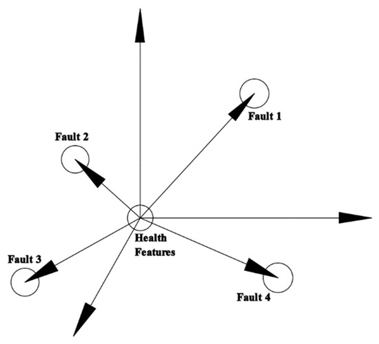
Figure 1. HF vector model.

Based on the analysis, this paper proposes an improved learning method utilizing dual-layer low-dimensional features extracted from multi-sensor vibration signals to effectively identify various faults in key components of roadheaders. Initially, a comparative sample set comprising fault and healthy signals from different sensor measuring points is constructed using time–frequency analysis. Subsequently, manifold learning is employed for initial low-dimensional feature extraction from the sample set, enabling differentiation between various fault and healthy signals at each measuring point and achieving preliminary fault discrimination. Moreover, the low-dimensional feature parameters from multiple sensors within the same timeframe are integrated to establish a pseudo-manifold network architecture that encompasses both temporal and spatial dimensions, facilitating further dimensionality reduction of the feature samples. The enhanced low-dimensional feature parameters are then extracted to achieve fault identification using multiple sensors. This multi-sensor, multi-layer enhanced manifold learning approach aims to enhance the differentiation of equipment vibration signals under different conditions through low-dimensional mapping, thereby improving the accuracy of fault classification and identification.

The flowchart of the proposed method is depicted in Figure 2, illustrating the three main steps in the feature extraction process. The first step involves dimensionality reduction of a multi-state sample set from a single sensor using locality-preserving projections (LPP). In the second step, mappings from multiple sensors are integrated to achieve fusion mapping. These separate mappings are derived individually from two-class models using LPP, with the goal of capturing and preserving local distinctions between each fault state and the normal state.

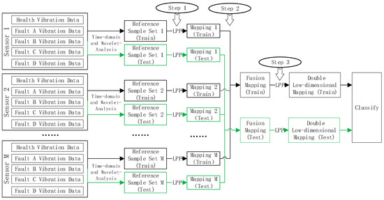
Figure 2. Flowchart of multi-sensor and multi-layer local projection for fault recognition of roadheader.

3. Construct the Reference Sample Set

3.1. Multi-Fault Vibration Signal Acquisition Experiment

This paper outlines a ground experiment conducted to gather diverse fault vibration signals from a roadheader. Modifications were made to the tunneling machine to simulate several typical underground faults, enabling the collection of vibration signals from its key components under varying conditions. The focal point of the experiment was an EBZ55 cantilever roadheader, which produced by Shijiazhuang Coal Mining Machinery Co., LTD of China (depicted in Figure 3). The experiment utilizes an MK920 piezoelectric vibration sensor produced by Wuxi Miko Sensor Technology Co., LTD of China, which operates with a power supply voltage range of 9–36 V. The sensor has a measurement range of 32 g and a sensitivity of 0.001 g, and it provides an output range of 0–10 V. The vibration signal acquisition device has the following technical specifications: a 12 V DC power supply, 24-bit AD resolution, and a maximum sampling frequency of 50 kHz.

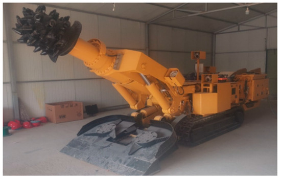
Figure 3. EBZ55 roadheader.

The experiment involved collecting vibration signals from the healthy state (Health) of the tunneling machine and from four common faults affecting the cutting mechanism. These faults are wear of the lifting cylinder bushing (Fault 1), misalignment between the output shaft of the reducer and the input shaft of the cutting head (Fault 2), excessive oil pressure (Fault 3), and electromagnetic valve failure (Fault 4). The sensor layout is illustrated in Figure 4 and detailed in Table 1.

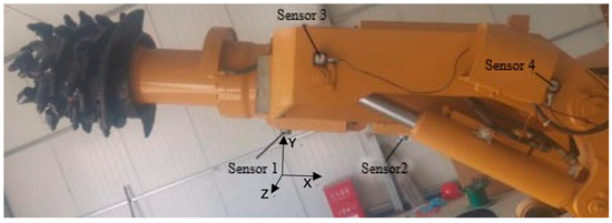
Figure 4. Actual layout of vibration sensors.

Table 1. Arrangement of measuring points.

Sensor	Position	Direction	Sensor	Position	Direction
1	Below the cutting reducer	Perpendicular to the lower surface of the cutting mechanism (Y)	4	Joint of turn table and cutting arm joint (left side).	Perpendicular to the left surface of the cutting mechanism (Z)
2	Below the cutting motor	Perpendicular to the lower surface of the cutting mechanism (Y)	5	Joint of the lifting cylinder and cutting arm (right side)	Perpendicular to the right surface of the cutting mechanism (Z)
3	Joint of the lifting cylinder and cutting arm (left side)	Perpendicular to the left surface of the cutting mechanism (Z)	6	Joint of turn table and cutting arm joint (right side).	Perpendicular to the right surface of the cutting mechanism (Z)

The vibration data acquisition experiment utilized a total of six sensors. The sampling frequency of the vibration signal is 10 kHz. Figure 5 depicts the vibration acceleration signals recorded by Sensor 1 during health operation of the roadheader.

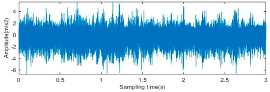
Figure 5. Vibration signal of Sensor 1.

3.2. Sample Construction Based on Time Domain and Wavelet Packet Transfer

Traditional vibration signal analysis involves extracting sensitive characteristics from vibration signals for comparison and experience summary using various data processing and statistical methods. In this study, characteristics extracted through traditional analysis (time–frequency features, frequency, and band energy) serve as the primary dataset for analysis.

Various time–frequency characteristic parameters of vibration signals are extracted, such as peak-to-peak value, effective value, absolute mean value, impulse factor, kurtosis value, crest factor, peak factor, waveform factor, and eight frequency band energy eigenvalues from the wavelet packet transform (WPT) method. These parameters are combined to form the characteristic parameter set of the vibration signal, as presented in Table 2.

Table 2. Characteristic parameter.

Time–Frequency Characteristics	Markup Symbols	Energy Ratios of Wavelet Analysis	Markup Symbols
Peak-to-peak	pk	Ratio 1	E1
Effective value	st	Ratio 2	E2
Absolute mean	me	Ratio 3	E3
Impulse factor	va	Ratio 4	E4
Kurtosis value	Kr	Ratio 5	E5
Margin factor	L	Ratio 6	E6
Peak factor	C	Ratio 7	E7
Waveform factor	S	Ratio 8	E8

The wavelet packet transform (WPT) is a widely recognized wavelet transform technique known for its properties of orthogonality, completeness, and time–frequency localization. Compared to the traditional discrete wavelet transform (DWT), WPT allows for further decomposition of signals in the high-frequency region, providing detailed information in addition to the approximation signal [21]. WPT is practically implemented using a series of recursive low-pass and high-pass wavelet filters (as depicted in Figure 6). In essence, the signal $S(t)$ undergoes iterative decomposition with the low-pass filter $h(k)$ and the high-pass filter $g(k)$.

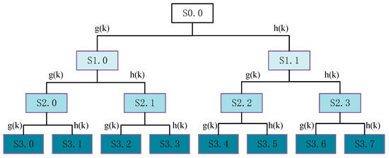
Figure 6. Illustration of WPT where, $S_{0,0}$ is the original signal; $S_{i,j}$ is the decomposed signal corresponding to the $j$ node of the $i$ layer.

The ratio $Ei$ of Table 2 is the energy of each sub-band signal $S_{i,j}$ [22].

The steps of frequency band energy feature extraction for wavelet packet decomposition are as follows.

(1)

Three layers of wavelet packet decomposition were performed for each group of vibration data, and the wavelet packet decomposition coefficients of eight sub-bands from low frequency to high frequency of the third layer were obtained.

$$\left(X_{3.0}, X_{3.1}, X_{3.2}, X_{3.3}, X_{3.4}, X_{3.5}, X_{3.6}, X_{3.7}\right)$$

(1)

(2)

The wavelet component analytical coefficients are reconstructed, and the signals in each sub-band range are extracted.

$$\begin{array}{ll}{S}_{0.0}& =S_{1.0}+S_{1.1}=S_{2.0}+S_{2.1}+S_{2.2}+S_{2.3}\\ & =S_{3.0}+S_{3.1}+S_{3.2}+S_{3.3}+S_{3.4}+S_{3.5}+S_{3.6}+S_{3.7}\end{array}$$

(2)

(3)

Calculate the energy of each sub-band:

$$Q_{3.i}={{\displaystyle \int \left|S_{3.i}\left(t\right)\right|}}^{2}dt={\displaystyle \sum _{h=0}^{h\in S}{\left|x_{i.h}\right|}^2}$$

(3)

where $i=0,1,2,3,4,5,6,7$ is the sub-band and $h=0,1,2\cdot \cdot \cdot n$ is the data of $S_{3.i}$

(4)

Normalize the energy of each sub-band:

$$E_i=Q_{3.i}/Q$$

(4)

where $Q={\displaystyle \sum _i^{i=7}{Q}_{3.i}}$ is the total energy sum of each energy band.

The resulting wavelet packet energy distribution is presented in Figure 7.

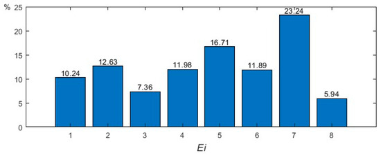
Figure 7. The result of WPT.

3.3. Reference Sample Sets Construction

Initially, we captured 32 sets of vibration signals from five types of operational states using a single sensor, with each signal lasting 3 s. We divided these into 16 groups for training data and 16 groups for testing data. Subsequently, the remaining five sensors collected an additional 5 × 32 sets of data over the same time period.

We extracted the characteristic parameters of the signal according to Table 2 and composed the characteristic sample $z_i$:

$$z_i=\left[pk,st,me,va,Kr,L,C,S,E1,E2\cdots E8\right];i=1,2,3\cdots 16$$

(5)

Then, the feature sample set of each operating state of a single sensor was established.

$$W_n=\left[Z_{n.0},Z_{n.1},Z_{n.2},Z_{n.3},Z_{n.4}\right]$$

(6)

where $n=1,2,3,4,5,6$ is the sensor.

$$Z_{n.m}=\left[z_1,z_2,\cdots z_{16}\right]$$

(7)

where $m=0,1,2,3,4$ is the operating state of the roadheader; 0 is the Health state, 1 is Fault 1, 2 is Fault 2, 3 is Fault 3, and 4 is Fault 4.

Finally, the reference characteristic sample sets $W_n\in R^{16\times 80}$ were formed.

4. Multi-Sensor and Multi-Layer Fault Recognition Based on LPP

4.1. Locality-Preserving Projection

Locality-preserving projection (LPP) is a manifold learning algorithm proposed by He based on the Laplacian eigenmaps (LE) algorithm [23]. This algorithm retains the advantages of non-linear manifold learning and linear learning, and its idea is to approximate the linear learning of LE. LPP can extract the most discriminative features for dimensionality reduction and is a dimensionality reduction method that preserves local information and reduces the interference of multiple external factors in signals, thereby preserving the local non-linear relationships when analyzing high-dimensional original data [24,25,26]. Compared with other non-linear dimensionality reduction methods, LPP can incorporate new analysis samples into the original manifold and find the corresponding mapping in the reduced subspace by calculation, thus enabling the LPP algorithm to evaluate and analyze new sample data.

The process of the LPP algorithm can be mainly divided into three steps [23,27,28,29,30]: (1) finding nearest neighbors; (2) computing the affinity matrix; and (3) constructing the objective function, as shown in Figure 8.

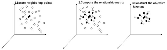
Figure 8. Flowchart of LPP.

The deduction process of LPP is as follows:

The original sample set is $X=\left\{x_1,x_2,x_3\dots x_n\right\}$, where the dimension of $X$ is $D$, $x_i\in R^D,i=0,1,2,\dots ,n$.

Then, $Y=\left\{y_1,y_2,y_3\dots y_n\right\}$ is the low-dimensional mapping of the original sample set in the manifold space, where the dimension of $Y$ is $d$, $d<<n$.

The objective function needs to be minimized when the LPP algorithm is used for low-dimensional mapping. After minimization, the original neighbor structure remains unchanged.

$$\arg \min {{\displaystyle \sum _{i,j=0}^n‖y_i-y_j‖}}^2{W}_{ij}$$

(8)

where $W_{ij}$ is the edge weight between $x_i$ and $x_j$ on the nearest neighbor graph $G$. For a neighbor graph $G$, if two vertices $j$ and $i$ are neighbors, $G_{i,j}=1$; otherwise, $G_{i,j}=0$. The formula for calculating the edge weights of the nearest neighbor graph is shown as follows:

$$W_{ij}=\left\{\begin{array}{c}{e}^{-{\displaystyle \frac{{‖x_i-x_j‖}^2}{t}}},G_{i,j}=1\\ 0,G_{i,j}=0\end{array}\right.$$

(9)

where $t$ is constant. By introducing the Heat–Kemal theory for calculation, the edge weight formula can be simplified as:

$$W_{ij}=\left\{\begin{array}{c}1,G_{i,j}=1\\ 0,G_{i,j}=0\end{array}\right.$$

(10)

The Laplace change is used to transform Formula (8).

$$\begin{array}{l}{{\displaystyle \sum _{i,j=0}^n‖y_i-y_j‖}}^2{W}_{ij}\\ ={\displaystyle \sum _{i,j=0}^n\left({y_i}^2+{y_j}^2-2y_i{y}_j\right)}{W}_{ij}\\ ={\displaystyle \sum _{i,j=0}^n{y_i}^2{W}_{ij}}+{\displaystyle \sum _{i,j=0}^n{y_j}^2{W}_{ij}}-2{\displaystyle \sum _{i,j=0}^n{y}_i{y}_j{W}_{ij}}\\ ={\displaystyle \sum _{i,j=0}^n{y_i}^2{D}_{ii}}+{\displaystyle \sum _{i,j=0}^n{y_j}^2{D}_{jj}}-2{\displaystyle \sum _{i,j=0}^n{y}_i{y}_j{W}_{ij}}\\ =2Y^{T}LY\end{array}$$

(11)

where $D_{ii}={\displaystyle {\sum }_j{W}_{ij}}$, $L$ is a Laplacian matrix, and $L=D-W$. Therefore, the objective function can be converted to the following formula:

$$\arg {\min }_{Y^{T}DY}{Y}^{T}LY$$

(12)

Using the Lagrange algorithm, Formula (12) can be converted to solve the eigenvalue problem of the following formula:

$$LY=\lambda DY$$

(13)

The low-dimensional space features of the original data can be obtained by solving Formula (13).

The LPP algorithm assumes that manifolds are linear, so

$$y_i=K^T{x}_i$$

(14)

By bringing Formulas (13) and (14) into Formula (11) for calculation, it can be concluded that:

$${{\displaystyle \sum _{i,j=0}^n‖y_i-y_j‖}}^2{W}_{ij}=2K^{T}XL{X}^{T}K$$

(15)

According to the constraints in the Laplacian feature mapping, it is obtained that:

$$K^{T}XD{X}^{T}K=1$$

(16)

Therefore, the objective function of LPP is as follows:

$$\arg {\min }_{K^{T}XD{X}^{T}K}{K}^{T}XL{X}^{T}K$$

(17)

Therefore, the most-mapped vector of the LPP algorithm can be obtained by finding the eigenvalue and eigenvector of the following formula:

$$XL{X}^{T}K=\lambda D{X}^{T}K$$

(18)

where $\lambda$ is the eigenvalue and $K$ represents the corresponding eigenvector. The first $d$ eigenvectors from $k_1,k_2,\dots ,k_l$ are associated with the $l$ smallest eigenvalue. Finally, the dimensionality reduction is as follows:

$$Y=K^{T}X\hspace{1em}K=[k_1,k_2,\dots ,k_d]$$

(19)

where $K$ is a $D\times d$ projection matrix. A reduced d-dimensional vector $y_i$ is received after the D-dimensional input $x_i$ is projected. The reduced vector $Y$ preserves the local variation information in regard to the relationship with its neighbors and will serve as the new feature. Therefore, LPP is able to seek the optimal linear locality structure embedded in that matrix, and the locality-preserving characteristic makes it relatively insensitive to isolated values and noise.

4.2. Reference Sample Set Analysis of Single Sensor

We use LPP manifold learning to perform dimensionality reduction on $W_n\in R^{16\times 80}$, where the reduced dimensionality $d=3$. Each sensor ultimately obtains an $LD{M}_n\in R^{3\times 80}$ low-dimensional mapping sample, and the analysis results of the training and test samples are shown in Figure 9 and Figure 10.

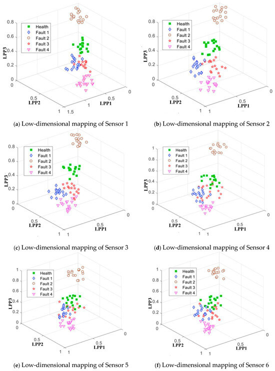
Figure 9. Low-dimensional mapping of training samples by LPP.

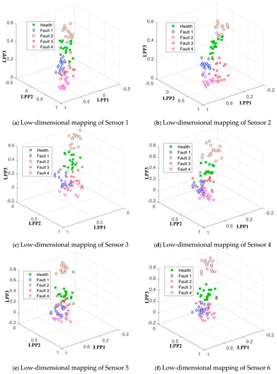
Figure 10. Low-dimensional mapping of test samples by LPP.

The low-dimensional mapping features of the two datasets can be examined. (1) The low-dimensional features of various operating states, while not entirely distinct from one another, exhibit a degree of clustering, with consistent clustering across different sensors. (2) Consistency is maintained to a certain extent in the behavior of the HF vector composed of each fault and health feature across all sensors. (3) Single-feature extraction alone may not suffice for distinguishing between fault categories.

4.3. Second-Layer Low-Dimensional Feature Extraction

Based on the analysis of the vibration data above, we obtained the low-dimensional mapping space for each sensor. While a single sensor can achieve some level of fault identification, its effectiveness is not particularly ideal. Moreover, the representations vary among sensors, but the HF vector for each fault remains nearly consistent across sensor directions. To address this, we utilize the low-dimensional spaces from six sensors for fusion, creating a multi-sensor fusion mapping.

$$Mapping={\left[{LD{M}_1}^T,{LD{M}_2}^T,{LD{M}_3}^T,{LD{M}_4}^T,{LD{M}_5}^T,{LD{M}_6}^T\right]}^T$$

$Mapping$ represents a pseudo-manifold in both spatial and temporal dimensions, constructed from low-dimensional features captured by six sensors across five states at 16 different time points. This feature set forms a spatial–temporal pseudo-manifold. When conducting further dimensionality reduction, it is crucial to preserve significant local spatial features and overarching characteristics across different states. Therefore, locality-preserving projection (LPP) is chosen to reduce dimensions in the fusion mapping process.

The fusion mappings are reduced in dimension by LPP learning, further purifying the manifold representation between samples. It can realize the depth enhancement processing of the difference of vibration signals in different states. Sensitive features extracted from enhanced shape features of the training samples and test samples are shown in Figure 11 and Figure 12.

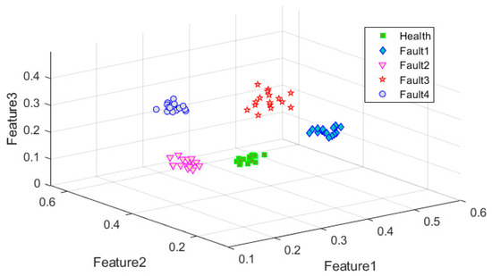
Figure 11. Double-layer low-dimensional feature (training sample).

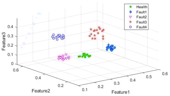
Figure 12. Double-layer low-dimensional feature (test sample).

Through the analysis of enhanced epidemic characteristics, the low-dimensional features of five operating states in the two groups of data were effectively distinguished; the same operating state showed good clustering, and the HF vector of the same fault showed good consistency in the two groups of analysis results.

4.4. KNN Classification

The enhanced feature analysis results are fed into the classifier for classification and recognition. The classification process typically involves two steps: the initial step utilizes known instance data for training, learning, and constructing a classifier under supervision, while the subsequent step employs the classifier’s test data for sample classification and recognition. As is evident in Figure 11 and Figure 12, the low-dimensional feature model exhibits clarity, with the overall data volume being modest, thereby eliminating the need for intricate operations. Consequently, k-nearest neighbors (KNN) stands out as the prevalent classification method. The fundamental concept of KNN classification is to choose the closest neighbor to the sample based on the distance from the sample to be partitioned and each training sample. Subsequently, the class of the sample is determined by these nearest neighbors. The computation process of KNN [30,31] involves (1) calculating the distances between the object to be classified and every object in the training set; (2) employing the Euclidean distance metric to define the nearest object as the nearest neighbor of the test object; and (3) categorizing the test object based on the attributes of these neighbors. The number of samples for each state in the sample set is 16, and thus we choose $k=12$.

This study employs low-dimensional features of training signals (shown as Figure 11) as KNN training sets, while low-dimensional features of test signals (shown as Figure 12) are used as the samples for classification. It is crucial to choose an appropriate value during the classification calculations.

The recognition rates for each operational state in the test signal sample are eventually obtained, as presented in Table 3. Following the application of the KNN classifier, only one sample in Fault 3 is misclassified as Fault 1, while the remainder are classified correctly. The overall recognition success rate across 80 samples stands at 98.75%

Table 3. Classification results of test signals.

Signal Category	Health	Fault 1	Fault 2	Fault 3	Fault 4
Sample Quantity	16	16	16	16	16
Classified Quantity	16	15	16	17	16
Recognition Rate (%)	100	93.75	100	93.75	100

5. Conclusions

Health monitoring and fault identification are crucial processes for assessing equipment health. This paper introduces a dimensionality reduction learning analysis method for fault identification of key components in roadheaders based on multi-sensor and multi-layer sensitive feature enhancement. Initially, multiple fault reference models are constructed for each sensor, and low-dimensional feature parameters are extracted to complete the first step of feature enhancement. The subsequent layer of sensitive feature enhancement involves fusing low-dimensional feature parameters from multiple sensors, establishing sensitive feature comparison samples, and utilizing locality-preserving projection (LPP) for analyzing and processing these samples to enhance the distinction between various faults. This two-level, joint-low-dimensional sensitive feature extraction process enhances and expands the differences in the original vibration features across different states. The integration of reference prevalence from each sensor in various states and the extraction of multi-layer low-dimensional sensitive features present a novel mode for double-layer, low-dimensional feature extraction. Due to insufficient underground vibration data for multiple faults, the effectiveness of enhanced learning could not be verified using actual production data. To address this, a multi-state vibration signal acquisition experiment was conducted in a ground test field, and the experimental data were analyzed. Using the KNN classifier for classification and learning of sensitive features, the test sample recognition success rate reached 98.75%. This method’s effectiveness in fault identification under complex loads was demonstrated.

References

- Wang, G.; Ren, S.; Pang, Y.; Qu, S.; Zheng, D. Development achievements of China’ s coal industry during the 13th Five-Year Plan period and implementation path of “dual carbon” target. Coal Sci. Technol. 2021, 49, 1–8. [Google Scholar]
- Gao, Y.; Wang, Y.; Wang, G.; Wang, Y.; Liu, H.; Chen, J.; Liang, D.; Wu, F. Exploration and study on the construction paths to green mine in coal enterprises to wards the goal of carbon peak and carbon neutrality. China Coal 2022, 48, 16–20. [Google Scholar]
- Zhang, P.; Li, S.; Qiu, S.; Gu, L.; Hu, X. Advance detection technology and development of fast intelligent roadway drivage. J. China Coal Soc. 2021, 46, 2158–2173. [Google Scholar]
- Xia, Z.; Junying, R.; Chengshan, C.; Caijin, X. Application of cantilever roadheader in tunnel construction. In IOP Conference Series: Earth and Environmental Science; IOP Publishing: Tokyo, Japan, 2019; Volume 330, p. 022023. [Google Scholar]
- Zhang, X.; Yang, W.; Xue, X.; Zhang, C.; Wan, J.; Mao, Q.; Lei, M.; Du, Y.; Ma, H.; Zhao, Y.; et al. Challenges and developing of the intelligent remote controlon roadheaders in coal mine. J. China Coal Soc. 2022, 47, 579–597. [Google Scholar]
- Wang, S.; Wu, M. Study on influencing factors and autonomous correction method of roadheader cutting trajectory. In Proceedings of the 2017 IEEE 2nd Information Technology, Networking, Electronic and Automation Control Conference (ITNEC), Chengdu, China, 15–17 December 2017; pp. 654–658. [Google Scholar]
- Tian, M.Q.; Wang, W.; Song, J.C.; Song, Y.; Yan, L.; Xia, Y. A dynamic load identification method for rock roadheaders based on wavelet packet and neural network. In Proceedings of the 2015 IEEE 10th Conference on Industrial Electronics and Applications (ICIEA), Auckland, New Zealand, 15–17 June 2015. [Google Scholar]
- Wei, W.; Mu-Qin, T.; Lin, Y.; Hua, Y.; Na, Z.; Hong, L. Dynamic Load Identification Method of Rock Roadheader Using Multineural Network and Evidence Theory. Coal Technol. 2018, 37, 228–231. [Google Scholar]
- Li, B.; Wang, R.; Li, B.; Zhang, K. Vertical Vibration Analysis and Simulation Study of Longitudinal Roadheader. Coal Mine Mach. 2014, 35, 40–42. [Google Scholar]
- Li, D.; Tian, M.; Song, J.; Bao, W.; Ma, Z. Denoising method of vibration signal of roadheader based on the optimal wavelet basis selection. Ind. Mine Autom. 2016, 42, 35–39. [Google Scholar]
- Cheng, X.-W.; Huang, J.-N.; Dong, Z.-F. Application of Wavelet Denoising for Vibration Signal of Roadheader. Coal Mine Mach. 2015, 36, 230–232. [Google Scholar]
- Seker, S.-E.; Ocak, I. Performance prediction of roadheaders using ensemble machine learning techniques. Neural Comput. Appl. 2019, 31, 1103–1116. [Google Scholar] [CrossRef]
- Liu, Q.; Zhang, C.; Wei, M.; Chen, Q.; Li, N. Fault Diagnosis of Cutting Arm of Roadheader Based on Optimized BP Neural Network. Coal Mine Mach. 2020, 41, 146–149. [Google Scholar]
- Gashler, M.; Ventura, D.; Martinez, T. Manifold Learning by Graduated Optimization; Institute of Electrical and Electronics Engineers (IEEE): New York, NY, USA, 2011; Volume 41, pp. 1458–1470. [Google Scholar]
- An, J.; Ai, P.; Liu, C.; Xu, S.; Liu, D. Deep Clustering Bearing Fault Diagnosis Method Based on Local Manifold Learning of an Autoencoded Embedding. IEEE Access. 2021, 9, 30154–30168. [Google Scholar] [CrossRef]
- Yao, B.; Peng, Z.; Wu, L.; Guan, Y. Rolling Element Bearing Fault Diagnosis Using Improved Manifold Learning. IEEE Access 2017, 5, 6027–6035. [Google Scholar] [CrossRef]
- Liu, H.; Wang, R.; Wu, G.; Zhang, Y. Diesel Engine Fault Diagnosis Based on Kernel Robust Manifold Nonnegative Matrix Factorization and Fusion Features. Comput. Sci. 2023, 50 (Suppl. S1), 894–901. [Google Scholar]
- Li, J.; Wu, Y.; Li, P.-y.; Zheng, X.; Xu, J.; Ju, X. TBM tunneling parameters prediction based on Locally Linear Embedding and Support Vector Regression. J. Zhejiang Univ. (Eng. Sci.) 2021, 55, 1426–1435. [Google Scholar]
- Ji, X.; Yang, Y.; Qu, Y.; Jiang, H.; Wu, M. Health Diagnosis of Roadheader Based on Reference Manifold Learning and Improved K-Means. Shock Vib. 2021, 2021, 6311795. [Google Scholar] [CrossRef]
- Zhao, X.; Chen, T.; Peng, Y.; Ye, B. The Transformation of Convolution Type of Wavelet Packet and Its’ Fast Algorith. Signal Process. 2002, 18, 543–546. [Google Scholar]
- Nie, X.; Huang, H.; Li, X.; Zhao, C.; Wu, Y. Research on Online Monitoring of Milling Chatter Based on Improved Wavelet Packet Energy Entropy and Threshold Adaptation. Chin. J. Sci. Instrum. 2024, 45, 227–238. [Google Scholar]
- He, X.; Niyogi, P. Locality preserving projections. In Advances in Neural Information Processing Systems; ACM: New York, NY, USA, 2003; Volume 16. [Google Scholar]
- Diwan, A.; Roy, A.-K.; Mitra, S.-K. Locality Preserving Projection Based Multiple Copy-Paste Forgery Detection. In Proceedings of the 2020 IEEE Applied Signal Processing Conference (ASPCON), Kolkata, India, 7–9 October 2020; pp. 158–162. [Google Scholar]
- Tang, B. Fault Diagnosis Model Based on Feature Compression with Orthogonal Locality Preserving Projection. Chin. J. Mech. Eng. 2011, 24, 891–908. [Google Scholar] [CrossRef]
- Dong, S.; Xu, X.; Liu, J.; Gao, Z. Rotating machine fault diagnosis based on locality preserving projection and back propagation neural network–support vector machine model. Meas. Control 2015, 48, 211–216. [Google Scholar] [CrossRef]
- Zheng, Z.; Huang, X.; Chen, Z.; He, X.; Liu, H.; Yang, J. Regression analysis of locality preserving projections via sparse penalty. Inf. Sci. 2015, 303, 1–14. [Google Scholar] [CrossRef]
- Geoffroy, H.; Berger, J.; Colange, B.; Lespinats, S.; Dutykh, D. The use of dimensionality reduction techniques for fault detection and diagnosis in an AHU unit: Critical assessment of its reliability. J. Build. Perform. Simul. 2023, 16, 249–267. [Google Scholar] [CrossRef]
- Shi, M.; Zhao, R.; Wu, Y.; He, T. Fault diagnosis of rotor based on Local-Global Balanced Orthogonal Discriminant Projection. Measurement 2021, 168, 108320. [Google Scholar] [CrossRef]
- Majdar, R.-S.; Ghassemian, H. Improved Locality Preserving Projection for Hyperspectral Image Classification in Probabilistic Framework. Int. J. Pattern Recognit. Artif. Intell. 2021, 35, 2150042. [Google Scholar] [CrossRef]
- Ma, L.; Crawford, M.M.; Tian, J. Local Manifold Learning-Based -Nearest-Neighbor for Hyperspectral Image Classification. IEEE Trans. Geosci. Remote Sens. 2010, 48, 4099–4109. [Google Scholar] [CrossRef]
- Weinberger, K.-Q.; Saul, L.-K. Distance Metric Learning for Large Margin Nearest Neighbor Classification. J. Mach. Learn. Res. 2009, 10, 207–244. [Google Scholar]
Disclaimer/Publisher’s Note: The statements, opinions and data contained in all publications are solely those of the individual author(s) and contributor(s) and not of MDPI and/or the editor(s). MDPI and/or the editor(s) disclaim responsibility for any injury to people or property resulting from any ideas, methods, instructions or products referred to in the content. |
© 2025 by the authors. Licensee MDPI, Basel, Switzerland. This article is an open access article distributed under the terms and conditions of the Creative Commons Attribution (CC BY) license (https://creativecommons.org/licenses/by/4.0/).