


Adaptive Neural-Network-Based Lossless Image Coder with Preprocessed Input Data


Abstract
1. Introduction
2. Scientific Background
2.1. Note on Lossless Image Coding Techniques
2.2. AdNNs vs. Deep Learning Approach
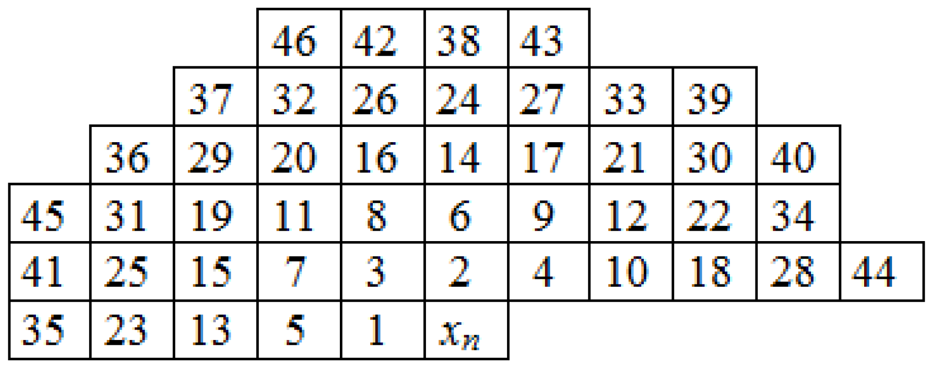
2.3. Note on Pixel Index Notation
3. Implemented Artificial Neural Network
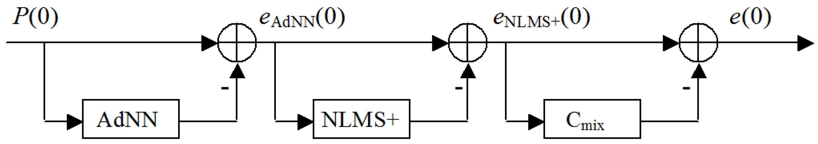
4. The Coder Structure
| Algorithm 1 Coder operation |
|
For each coded pixel : |
| Algorithm 2 Decoder operation |
|
For each coded pixel prediction error : |
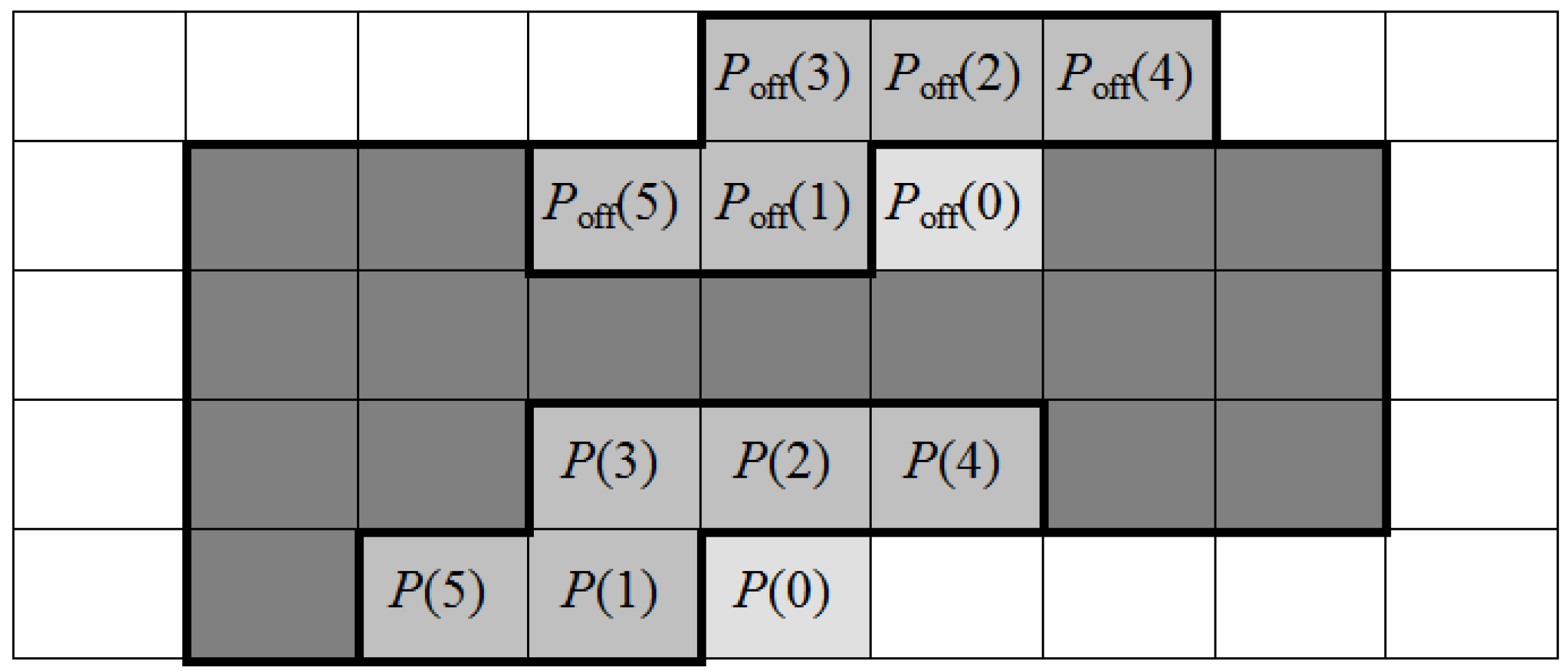
5. Preprocessing Data for AdNN
5.1. Concept 1
5.2. Concept 2
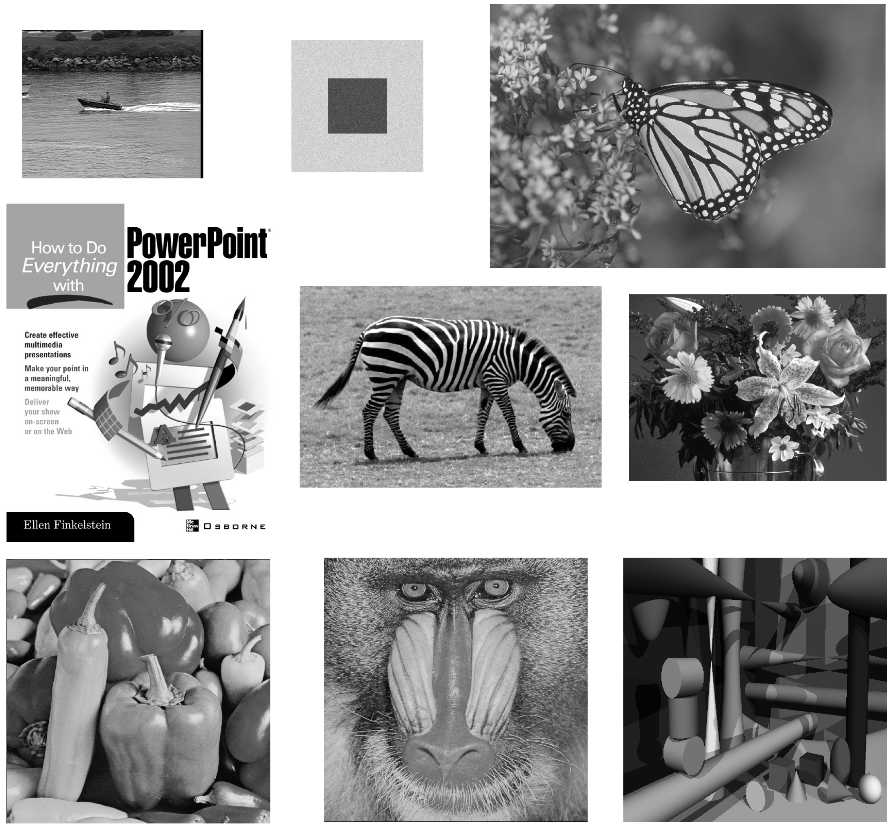
6. Experiments

| Images | JPEG-LS [1] | CALIC [4] | TS-FNN [37] | AdNN [14] | AdNN+ [16] | C1 | C2 |
|---|---|---|---|---|---|---|---|
| Camera | 4.31 | 4.190 | 4.39 | 4.13 | 4.120 | 4.007 | 3.999 |
| Couple256 | 3.70 | 3.609 | 3.73 | 3.60 | 3.561 | 3.435 | 3.441 |
| Noisesquare | 5.68 | 5.443 | 5.44 | 5.18 | 5.201 | 5.166 | 5.135 |
| Airplane | 3.82 | 3.743 | 3.68 | 4.06 | 3.598 | 3.557 | 3.558 |
| Baboon | 6.04 | 5.875 | 5.97 | 5.77 | 5.706 | 5.662 | 5.641 |
| Lennagrey | 4.24 | 4.102 | 4.08 | 3.97 | 3.925 | 3.899 | 3.890 |
| Peppers | 4.51 | 4.421 | 4.33 | 4.27 | 4.201 | 4.153 | 4.146 |
| Shapes | 1.21 | 1.139 | 1.79 | 1.44 | 1.708 | 1.111 | 1.124 |
| Balloon | 2.90 | 2.825 | 2.54 | 2.80 | 2.647 | 2.602 | 2.577 |
| Barb | 4.69 | 4.413 | 4.49 | 4.16 | 3.868 | 3.843 | 3.821 |
| Gold Hill | 4.48 | 4.394 | 4.36 | 4.33 | 4.238 | 4.196 | 4.192 |
| Mean | 4.144 | 4.014 | 4.073 | 3.974 | 3.888 | 3.785 | 3.775 |
| Images | LCIC | JPEG 2000 | JPEG-LS | JPEG-XL | FLIF | WebP | L3C | CWP LIC | LCIC Duplex | C1 | C2 |
|---|---|---|---|---|---|---|---|---|---|---|---|
| Airplane | 3.99 | 4.00 | 3.80 | 3.71 | 3.82 | 3.87 | 4.56 | 3.69 | 3.69 | 3.533 | 3.532 |
| Barbara | 4.61 | 4.61 | 4.70 | 4.40 | 4.56 | 4.55 | 5.44 | 4.35 | 4.36 | 3.850 | 3.828 |
| Coastguard | 4.82 | 4.83 | 4.86 | 4.73 | 4.93 | 4.81 | 5.82 | 4.80 | 4.83 | 4.351 | 4.368 |
| Comic | 5.63 | 5.65 | 5.30 | 5.07 | 5.50 | 5.45 | 6.60 | 4.83 | 4.83 | 4.861 | 4.873 |
| Flowers | 4.91 | 4.92 | 4.62 | 4.51 | 4.74 | 4.76 | 5.53 | 4.41 | 4.35 | 4.318 | 4.327 |
| Goldhill | 4.58 | 4.59 | 4.43 | 4.37 | 4.50 | 4.47 | 5.27 | 4.33 | 4.33 | 4.143 | 4.143 |
| Lennagrey | 4.31 | 4.31 | 4.24 | 4.16 | 4.28 | 4.14 | 4.95 | 4.13 | 4.08 | 3.899 | 3.890 |
| Mandrill | 6.11 | 6.11 | 6.04 | 5.98 | 6.14 | 5.89 | 6.97 | 5.95 | 5.89 | 5.663 | 5.643 |
| Monarch | 3.82 | 3.82 | 3.70 | 3.54 | 3.68 | 3.73 | 4.37 | 3.40 | 3.45 | 3.368 | 3.342 |
| Pepper | 4.63 | 4.63 | 4.51 | 4.48 | 4.58 | 4.50 | 5.38 | 4.67 | 4.38 | 4.146 | 4.140 |
| Ppt3 | 2.41 | 2.41 | 2.04 | 1.84 | 1.87 | 2.06 | 3.71 | 2.14 | 2.07 | 1.770 | 1.775 |
| Zebra | 4.89 | 4.89 | 4.81 | 4.66 | 4.84 | 4.86 | 6.08 | 4.65 | 4.68 | 4.347 | 4.339 |
| Mean | 4.559 | 4.564 | 4.421 | 4.288 | 4.453 | 4.424 | 5.390 | 4.279 | 4.245 | 4.021 | 4.017 |
7. Conclusions
Author Contributions
Funding
Institutional Review Board Statement
Informed Consent Statement
Data Availability Statement
Conflicts of Interest
References
- Weinberger, M.; Seroussi, G.; Sapiro, G. The LOCO-I lossless image compression algorithm: Principles and standardization into JPEG-LS. IEEE Trans. Image Process. 2000, 9, 1309–1324. [Google Scholar] [CrossRef]
- Marcellin, M.; Gormish, M.; Bilgin, A.; Boliek, M. An overview of JPEG-2000. In Proceedings of the Proceedings DCC 2000. Data Compression Conference, Snowbird, UT, USA, 28–30 March 2000; pp. 523–541. [Google Scholar] [CrossRef]
- Codec WebP 1.3. Available online: https://storage.googleapis.com/downloads.webmproject.org/releases/webp/libwebp-1.3.0-windows-x64.zip (accessed on 8 April 2023).
- Wu, X.; Memon, N. CALIC—A Context Based Adaptive Lossless Image Codec. In Proceedings of the 1996 IEEE International Conference on Acoustics, Speech, and Signal Processing Conference Proceedings, Atlanta, GA, USA, 9 May 1996; Volume 4, pp. 1890–1893. [Google Scholar] [CrossRef]
- Meyer, B.; Tischer, P. TMWLego—An Object Oriented Image Modeling Framework. In Proceedings of the Data Compression Conference, Washington, DC, USA, 27–29 March 2001; p. 504. [Google Scholar]
- Ye, H.; Deng, G.; Devlin, J. A weighted least squares method for adaptive prediction in lossless image compression. In Proceedings of the Picture Coding Symposium PCS’03, Saint Malo, France, 23–25 April 2003; pp. 489–493. [Google Scholar]
- Matsuda, I.; Ozaki, N.; Umezu, Y.; Itoh, S. Lossless coding using Variable Blok-Size adaptive prediction optimized for each image. In Proceedings of the 13th European Signal Processing Conference EUSIPCO-05 CD, Antalya, Turkey, 4–8 September 2005. [Google Scholar]
- Dai, W.; Xiong, H.; Wang, J.; Zheng, Y. Large Discriminative Structured Set Prediction Modeling with Max-Margin Markov Network for Lossless Image Coding. IEEE Trans. Image Process. 2014, 23, 541–554. [Google Scholar] [CrossRef]
- Matsuda, I.; Ozaki, N.; Umezu, Y.; Itoh, S. A Lossless Image Coding Method Based on Probability Model Optimization. In Proceedings of the 2018 26th European Signal Processing Conference (EUSIPCO), Rome, Italy, 3–7 September 2018; pp. 156–160. [Google Scholar]
- Unno, K.; Kameda, Y.; Matsuda, I.; Itoh, S.; Naito, S. Lossless Image Coding Exploiting Local and Non-local Information via Probability Model Optimization. In Proceedings of the 27th European Signal Processing Conference (EUSIPCO), A Coruna, Spain, 2–6 September 2019; pp. 1–5. [Google Scholar]
- Kojima, H.; Kita, Y.; Matsuda, I.; Itoh, S.; Kameda, Y.; Unno, K.; Kawamura, K. Improved Probability Modeling for Lossless Image Coding Using Example Search and Adaptive Prediction. In Proceedings of the International Workshop on Advanced Imaging Technology (IWAIT) 2022, Hong Kong, China, 4–6 January 2022. [Google Scholar]
- Ulacha, G.; Stasinski, R.; Wernik, C. Extended Multi WLS Method for Lossless Image Coding. Entropy 2020, 22, 919. [Google Scholar] [CrossRef] [PubMed]
- Kau, L.J.; Lin, Y.P.; Lin, C.T. Lossless image coding using adaptive, switching algorithm with automatic fuzzy context modelling. IEE Proc.-Vision Image Signal Process. 2006, 153, 684–694. [Google Scholar] [CrossRef]
- Marusic, S.; Deng, G. A neural network based adaptive non-linear lossless predictive coding technique. In Proceedings of the ISSPA ’99. Proceedings of the Fifth International Symposium on Signal Processing and Its Applications (IEEE Cat. No.99EX359), Brisbane, QLD, Australia, 22–25 August 1999; Volume 2, pp. 653–656. [Google Scholar] [CrossRef]
- Marusic, S.; Deng, G. Adaptive prediction for lossless image compression. Signal Process. Image Commun. 2002, 17, 363–372. [Google Scholar] [CrossRef]
- Ulacha, G.; Stasiński, R. Improving Neural Network Approach to Lossless Image Coding. In Proceedings of the 29th Picture Coding Symposium PCS’12, Krakow, Poland, 7–9 May 2012; pp. 173–176. [Google Scholar]
- Rhee, H.; Jang, Y.I.; Kim, S.; Cho, N.I. Lossless Image Compression by Joint Prediction of Pixel and Context Using Duplex Neural Networks. IEEE Access 2021, 9, 86632–86645. [Google Scholar] [CrossRef]
- Zhang, Z.; Wang, H.; Chen, Z.; Liu, S. Learned Lossless Image Compression Based on Bit Plane Slicing. In Proceedings of the 2024 IEEE/CVF Conference on Computer Vision and Pattern Recognition (CVPR), Seattle, WA, USA, 16–22 June 2024; pp. 27569–27578. [Google Scholar] [CrossRef]
- Rhee, H.; Cho, N.I. Resolution-Adaptive Lossless Image Compression Using Frequency Decomposition Network. In Proceedings of the 2023 Asia Pacific Signal and Information Processing Association Annual Summit and Conference (APSIPA ASC), Taipei, Taiwan, 31 October–3 November 2023. [Google Scholar] [CrossRef]
- Feng, X.; Gu, E.; Zhang, Y.; Li, A. Probability Prediction Network With Checkerboard Prior for Lossless Remote Sensing Image Compression. IEEE J. Sel. Top. Appl. Earth Obs. Remote Sens. 2024, 17, 17971–17982. [Google Scholar] [CrossRef]
- Shen, Y.; Wu, G.; Swaminathan, V.; Wang, H.; Petrangeli, S.; Yu, T. GPU-accelerated Lossless Image Compression with Massive Parallelization. In Proceedings of the 2023 IEEE International Symposium on Multimedia (ISM), Laguna Hills, CA, USA, 11–13 December 2023; pp. 321–324. [Google Scholar] [CrossRef]
- Said, A.; Le, H.; Farhadzadeh, F. Bitstream Organization for Parallel Entropy Coding on Neural Network-based Video Codecs. In Proceedings of the 2023 IEEE International Symposium on Multimedia (ISM), Laguna Hills, CA, USA, 11–13 December 2023; pp. 1–9. [Google Scholar] [CrossRef]
- Bai, Y.; Liu, X.; Wang, K.; Ji, X.; Wu, X.; Gao, W. Deep Lossy Plus Residual Coding for Lossless and Near-Lossless Image Compression. IEEE Trans. Pattern Anal. Mach. Intell. 2024, 46, 3577–3594. [Google Scholar] [CrossRef] [PubMed]
- Zhang, S.; Zhang, C.; Kang, N.; Li, Z. Numerical Invertible Volume Preserving Flow for Efficient Lossless Compression. In Proceedings of the 2021 IEEE/CVF Conference on Computer Vision and Pattern Recognition (CVPR), Nashville, TN, USA, 20–25 June 2021; pp. 1–10. [Google Scholar] [CrossRef]
- Mishra, D.; Singh, S.K.; Singh, R.K. Deep Architectures for Image Compression: A Critical Review. Signal Process. 2022, 191, 108346. [Google Scholar] [CrossRef]
- Aiazzi, B.; Baronti, S.; Alparone, L. Near-lossless image compression by relaxation-labeled prediction. Signal Process. 2002, 82, 1619–1631. [Google Scholar] [CrossRef]
- Golchin, F.; Paliwal, K.K. Classified adaptive prediction and entropy coding for lossless coding of images. In Proceedings of the International Conference on Image Processing, Santa Barbara, CA, USA, 26–29 October 1997; pp. 110–113. [Google Scholar]
- Meyer, B.; Tischer, P. TMW—A new method for lossless image compression. In Proceedings of the International Picture Coding Symposium (PCS 97), Berlin, Germany, 10–12 September 1997; pp. 533–538. [Google Scholar]
- Strutz, T. Context-based adaptive linear prediction for Lossless Image Coding. In Proceedings of the 4th International ITG Conference on Source and Channel Coding, Berlin, Germany, 28–30 January 2002; pp. 105–109. [Google Scholar]
- Strutz, T. Context-Based Predictor Blending for Lossless Colour Image Compression. IEEE Trans. Circuits Syst. Video Technol. 2016, 26, 687–695. [Google Scholar] [CrossRef]
- Ulacha, G.; Stasiński, R. New Context-Based Adaptive Linear Prediction Algorithm for Lossless Image Coding. In Proceedings of the 2014 International Conference on Signals and Electronic Systems (ICSES), Poznan, Poland, 11–13 September 2014; pp. 1–4. [Google Scholar]
- Ulacha, G.; Stasinski, R. Context based lossless coder based on RLS predictor adaption scheme. In Proceedings of the 2009 16th IEEE International Conference on Image Processing (ICIP), Cairo, Egypt, 7–10 November 2009; pp. 1917–1920. [Google Scholar] [CrossRef]
- Wu, X.; Barthel, E.; Zhang, W. Piecewise 2D autoregression for predictive image coding. In Proceedings of the Proceedings 1998 International Conference on Image Processing. ICIP98 (Cat. No.98CB36269), Chicago, IL, USA, 7 October 1998; Volume 3, pp. 901–904. [Google Scholar] [CrossRef]
- Ye, H.; Deng, G.; Devlin, J. Adaptive linear prediction for lossless coding of greyscale images. In Proceedings of the Proceedings 2000 International Conference on Image Processing (Cat. No.00CH37101), Vancouver, BC, Canada, 10–13 September 2000; Volume 1, pp. 128–131. [Google Scholar] [CrossRef]
- Ye, H.; Deng, G.; Devlin, J. Least squares approach for lossless image coding. In Proceedings of the ISSPA ’99. Proceedings of the Fifth International Symposium on Signal Processing and Its Applications (IEEE Cat. No.99EX359), Brisbane, QLD, Australia, 22–25 August 1999; Volume 1, pp. 63–66. [Google Scholar] [CrossRef]
- Takizawa, K.; Takenouchi, S.; Aomori, H.; Otake, T.; Tanaka, M.; Matsuda, I.; Itoh, S. Lossless image coding by cellular neural networks with minimum coding rate learning. In Proceedings of the 2011 20th European Conference on Circuit Theory and Design (ECCTD), Brisbane, QLD, Australia, 10–15 June 2011; pp. 33–36. [Google Scholar] [CrossRef]
- Lee, C.H.; Kau, L.J.; Lin, Y.P. A fuzzy neural network based adaptive predictor with P-controller compensation for lossless compression of images. In Proceedings of the 2009 IEEE International Symposium on Circuits and Systems (ISCAS), Taipei, Taiwan, 24–27 May 2009; pp. 633–636. [Google Scholar]
- Rahman, A.; Hamada, M.; Rahman, A. A comparative analysis of the state-of-the-art lossless image compression techniques. In Proceedings of the 4th ETLTC International Conference on ICT Integration in Technical Education (ETLTC2022), Aizuwakamatsu, Japan, 25–28 January 2022. [Google Scholar]
- Mentzer, F.; van Gool, L.; Tschannen, M. Learning Better Lossless Compression Using Lossy Compression. In Proceedings of the 2020 IEEE/CVF Conference on Computer Vision and Pattern Recognition (CVPR), Seattle, WA, USA, 13–19 June 2020; pp. 6637–6646. [Google Scholar]
- Rhee, H.; Jang, Y.I.; Kim, S.; Cho, N.I. Learned Lossless Image Compression with Frequency Decomposition Network. In Proceedings of the 2022 IEEE/CVF Conference on Computer Vision and Pattern Recognition (CVPR), New Orleans, LA, USA, 18–24 June 2022; pp. 6023–6032. [Google Scholar]
- Hoogeboom, E.; Peters, J.W.; van den Berg, R.; Welling, M. Integer Discrete Flows and Lossless Compression. In Proceedings of the International Conference on Neural Information Processing Systems (2019), Vancouver, BC, Canada, 8–14 December 2019. [Google Scholar]
- Mentzer, F.; Agustsson, E.; Tschannen, M.; Timofte, R.; Gool, L.V. Practical Full Resolution Learned Lossless Image Compression. In Proceedings of the 2019 IEEE/CVF Conference on Computer Vision and Pattern Recognition (CVPR), Long Beach, CA, USA, 15–20 June 2019. [Google Scholar] [CrossRef]
- Cao, S.; Wu, C.-Y.; Krähenbühl, P. Lossless Image Compression through Super-Resolution. arXiv 2020, arXiv:2004.02872. [Google Scholar] [CrossRef]
- Shim, J.H.; Rhee, H.; Jang, Y.I.; Lee, G.; Kim, S.; Cho, N.I. Lossless Image Compression Based on Image Decomposition and Progressive Prediction Using Convolutional Neural Networks. In Proceedings of the 2021 Asia-Pacific Signal and Information Processing Association Annual Summit and Conference (APSIPA ASC), Tokyo, Japan, 14–17 December 2021; pp. 158–163. [Google Scholar]
- Gumus, S.; Kamisli, F. A Learned Pixel-by-Pixel Lossless Image Compression Method with 59K Parameters and Parallel Decoding. arXiv 2022, arXiv:2212.01185. [Google Scholar]
- Ulacha, G.; Stasiński, R. A Time-Effective Lossless Coder Based on Hierarchical Contexts and Adaptive Predictors. In Proceedings of the 14th IEEE Mediterranean Electrotechnical Conference MELECON’08, Ajaccio, France, 5–7 May 2008; pp. 829–834. [Google Scholar]
- Ulacha, G.; Łazoryszczak, M. Lossless Image Coding Using Non-MMSE Algorithms to Calculate Linear Prediction Coefficients. Entropy 2023, 25, 156. [Google Scholar] [CrossRef]
- Liang, Y.; Jia, T.; Li, N.; Liu, X.; Jiang, J.; Lu, G. Review of Static Image Compression Algorithms. In Proceedings of the 2024 IEEE 7th Advanced Information Technology, Electronic and Automation Control Conference (IAEAC), Chongqing, China, 15–17 March 2024; pp. 222–231. [Google Scholar] [CrossRef]
- Test Images. Available online: https://kakit.zut.edu.pl/fileadmin/Test_Images.zip (accessed on 20 December 2024).

| j | j | j | |||
|---|---|---|---|---|---|
| 1 | 7 | 13 | |||
| 2 | 8 | 14 | |||
| 3 | 9 | 15 | |||
| 4 | 10 | 16 | |||
| 5 | 11 | 17 | |||
| 6 | 12 | 18 |
Disclaimer/Publisher’s Note: The statements, opinions and data contained in all publications are solely those of the individual author(s) and contributor(s) and not of MDPI and/or the editor(s). MDPI and/or the editor(s) disclaim responsibility for any injury to people or property resulting from any ideas, methods, instructions or products referred to in the content. |
© 2025 by the authors. Licensee MDPI, Basel, Switzerland. This article is an open access article distributed under the terms and conditions of the Creative Commons Attribution (CC BY) license (https://creativecommons.org/licenses/by/4.0/).
Share and Cite
Ulacha, G.; Stasinski, R. Adaptive Neural-Network-Based Lossless Image Coder with Preprocessed Input Data. Appl. Sci. 2025, 15, 2603. https://doi.org/10.3390/app15052603
Ulacha G, Stasinski R. Adaptive Neural-Network-Based Lossless Image Coder with Preprocessed Input Data. Applied Sciences. 2025; 15(5):2603. https://doi.org/10.3390/app15052603
Chicago/Turabian StyleUlacha, Grzegorz, and Ryszard Stasinski. 2025. "Adaptive Neural-Network-Based Lossless Image Coder with Preprocessed Input Data" Applied Sciences 15, no. 5: 2603. https://doi.org/10.3390/app15052603
APA StyleUlacha, G., & Stasinski, R. (2025). Adaptive Neural-Network-Based Lossless Image Coder with Preprocessed Input Data. Applied Sciences, 15(5), 2603. https://doi.org/10.3390/app15052603