Deep Learning Algorithm for Automatic Classification of Power Quality Disturbances

Abstract

Power quality disturbances (PQDs) are major obstacles to maintaining the reliability and stability of electrical systems. This study introduces a new multi-scale deep learning method to classify PQDs, aiming to enhance the accuracy and efficiency of power quality (PQ) analysis and monitoring systems. By combining 1-D convolutional neural networks (CNNs) with an attention mechanism, this approach overcomes the limitations of traditional techniques. Moreover, varying-size convolutional layers allow for the direct learning of complex patterns and features from PQ signals. To address the challenge of limited labeled PQ datasets, this research utilizes an open-source dataset generator to create large-scale datasets with annotated PQDs. Through a comparison with existing models in the field, the superiority of the proposed CNN-based approach is evident, achieving an accuracy level of up to $99.49\%$. The results demonstrate promising classification performance in terms of simplicity and accuracy, highlighting the potential of this approach to improve PQ analysis and disturbance identification.

1. Introduction

The increasing reliance on electrical power for various aspects of modern society has made PQ a critical concern. Maintaining high PQ is essential to ensure the reliable operation of electrical devices and minimize the risk of equipment failure or power system instability. PQ events, such as voltage sags, swells, and transients, can have significant negative impacts on the performance and lifespan of electrical equipment. Therefore, early identification and mitigation of PQ issues is crucial.

Traditional methods for detecting, classifying, and localizing PQ events have limitations in terms of accuracy, robustness, and computational efficiency. Recent advancements in machine learning (ML) and artificial intelligence (AI) offer promising solutions to overcome these limitations [1,2]. This research aims to develop and evaluate a novel ML algorithm for the automatic classification of PQ events. By leveraging the power of advanced data-driven techniques, the proposed research seeks to improve the monitoring and maintenance of PQ in modern power systems, ultimately enhancing the reliability and stability of the electrical grid.

PQ, a measure of the consistency and reliability of the voltage, current, and frequency of an electrical power system, is an essential factor in the operation of modern power systems [3,4]. The growing integration of renewable energy sources, proliferation of non-linear loads, and increasing reliance on sensitive electronic devices have resulted in increased susceptibility to PQ issues. PQ events, such as voltage sags, swells, transients, harmonics, and flickers, can adversely affect the performance, safety, and lifespan of electrical equipment, leading to increased energy losses, equipment downtime, and maintenance costs. In extreme cases, these events can even cause power system instability or failure, posing risks to public safety and the economy [5,6,7].

Recent advancements in ML and AI offer promising alternatives to traditional PQ analysis techniques. ML and AI algorithms have demonstrated their potential in various domains, including image recognition, natural language processing, and autonomous systems, owing to their ability to learn complex patterns and adapt to different scenarios [8,9,10]. The application of these advanced data-driven techniques to PQ event detection, classification, and localization has the potential to overcome the limitations of traditional methods and enable more accurate, efficient, and reliable PQ monitoring and maintenance.

The motivation behind this research is to explore and exploit the capabilities of ML and AI algorithms for the automatic detection, classification, and localization of PQ events. By developing and evaluating algorithms that can accurately identify and classify PQ events, this research aims to contribute to the identification and mitigation of PQ issues in modern power systems. This work seeks to enhance the electrical grid’s overall reliability, stability, and efficiency, minimizing the negative impacts of PQ events on equipment, businesses, and consumers. Ultimately, this research aims to push the boundaries of PQ analysis and contribute to the development of more intelligent and resilient power systems for the future.

Hence, this paper introduces a novel deep learning approach for PQDs classification. The main contributions of this study are:

• This study introduces a novel deep learning approach for classifying PQDs. By integrating CNNs with attention mechanisms, the proposed method aims to improve the accuracy and efficiency of PQ analysis and monitoring systems.
• Introducing a multi-scale convolutional network that employs multiple convolutional layers with varying kernel sizes, allowing it to effectively capture feature patterns across different scales of PQDs.
• When comparing the introduced CNN approach with other state-of-the-art methods, the results demonstrate promising classification performance. The introduced deep learning approach balances simplicity and accuracy, showcasing its potential to enhance PQ analysis.

The rest of the article is organized as follows: Section 2 briefly reviews some background knowledge. Section 3 illustrates the proposed deep learning CNN architecture. Section 4 discusses the experimental results. Finally, Section 5 presents the conclusions and future work.

2. Related Work

PQDs refer to variations or deviations in the electrical characteristics of power systems that can impact the performance and reliability of electrical devices [6]. Common PQDs include the following:

• Voltage sag refers to a short-term dip in voltage below the normal operating level. It typically lasts for a few cycles and can be caused by faults, starting large motors, or sudden changes in load. Voltage sags can lead to equipment malfunctions, flickering lights, or temporary disruptions in device operation.
• Voltage swells are short-term increases in voltage magnitude above the normal level. Like voltage sags, voltage swells can occur due to various factors such as faults, load switching, or capacitor bank energization. Voltage swells can cause damage to sensitive electronic equipment, premature aging of devices, or excessive current flow.
• Harmonics are additional sinusoidal waveforms that have frequencies that are integer multiples of the fundamental frequency (typically 50 Hz or 60 Hz). Harmonics are caused by non-linear loads such as power electronics, variable speed drives, or rectifiers. They can distort the voltage and current waveforms, leading to overheating of equipment, increased losses, and interference with communication systems.
• Transients, also known as voltage spikes or surges, are brief and abrupt changes in voltage magnitude that can occur due to lightning strikes, switching operations, or equipment faults. Transients can have high amplitudes and short durations, potentially causing damage to sensitive devices, data loss, or disruption of operations.
• Interruptions refer to complete power loss or a sudden stoppage of the supply voltage. They can be caused by faults in the power system, equipment failures, or intentional switching. Interruptions can lead to unexpected shutdowns, loss of data, or disruption of critical processes.
• Flicker is the fluctuation of the perceived brightness of lights due to rapid changes in voltage. It can occur when large loads are switched on or off or during the operation of arc furnaces or welding equipment. Flicker can be visually disturbing and might affect the performance of sensitive equipment or human comfort.

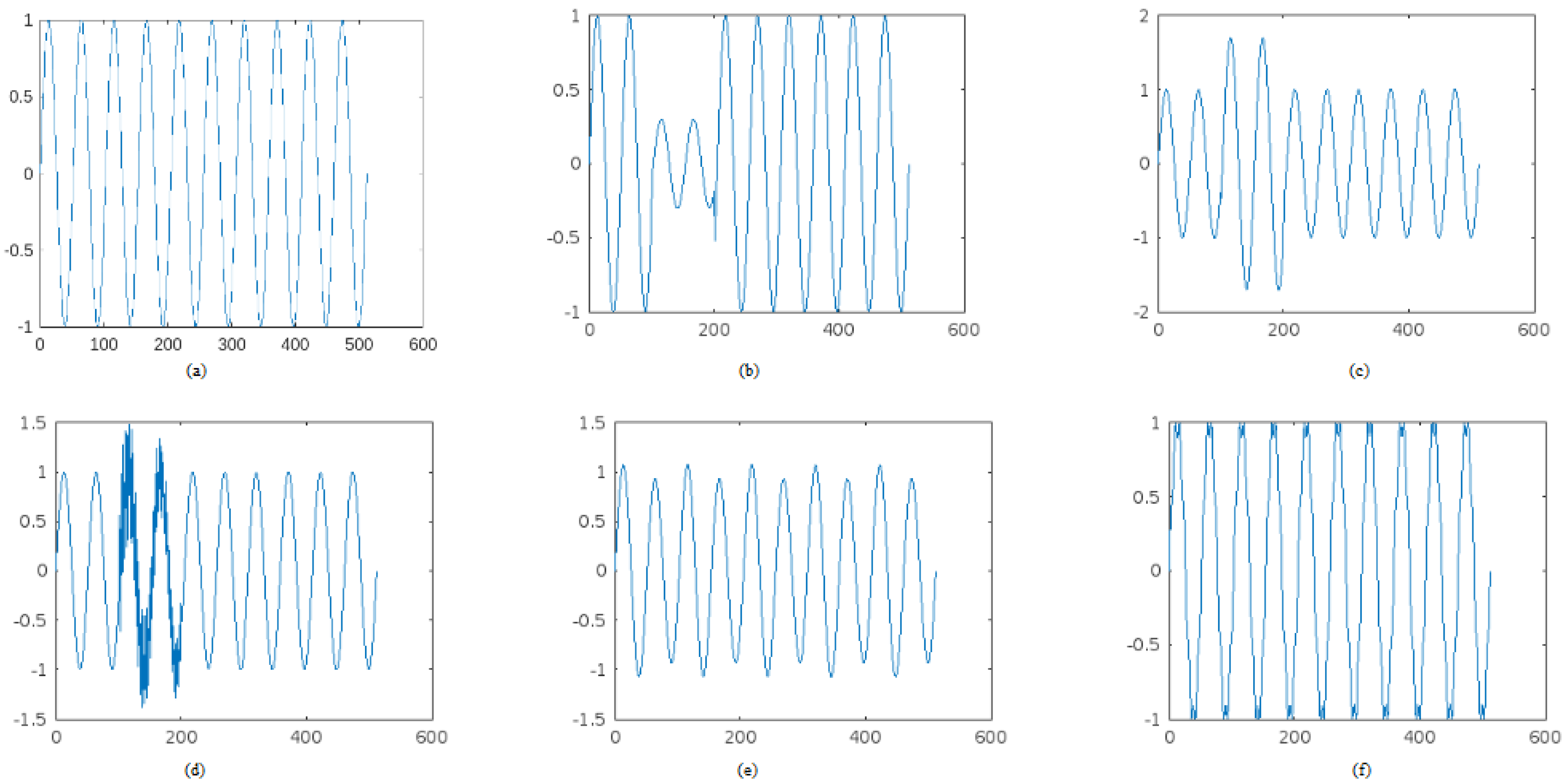
Other types of PQDs can include frequency variations, voltage unbalance, and voltage harmonics beyond the 50th or 100th order. Understanding and mitigating these PQDs is crucial for maintaining the reliability and efficiency of electrical systems and ensuring the proper functioning of connected devices. Figure 1 provides different PQD signals.

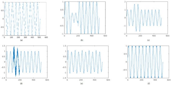
Figure 1. Different PQD Signals. (a) Normal signal. (b) Sag. (c) Swell. (d) Transient. (e) Flicker. (f) Harmonics.

Open-source dataset generators were developed as valuable tools for creating PQD datasets, as introduced by Machlev et al. [7]. These generators offer flexibility in controlling disturbance characteristics, including magnitude, duration, and frequency content. Moreover, the researchers recognized the effectiveness of deep learning classifiers, particularly CNNs, for PQD classification.

Wang and Chen [11] proposed a novel closed-loop approach using a deep CNN model for PQD classification. Their model incorporates a unique unit construction that includes 1-D convolutional layers, pooling, and batch normalization, facilitating multi-scale feature extraction while reducing overfitting.

ResNet50, a deep CNN architecture, has gained significant attention in image and signal analysis due to its ability to effectively learn deep features while mitigating the vanishing gradient problem through skip connections. Recent studies have leveraged ResNet50 for classifying power quality disturbances effectively. For instance, Jamlus et al. [12] utilized ResNet50 to analyze power quality signals, demonstrating accuracy and robustness. Their findings emphasized the ability of ResNet50 to extract relevant features from complex time-series data. While ResNet is a powerful architecture with several advantages, it does have some limitations, such as its increased depth. While beneficial for learning complex features, it can also lead to increased computational complexity. Moreover, these networks may be more prone to overfitting, especially when dealing with smaller datasets.

A hybrid technique combining ML algorithms with wavelet-based feature extraction methods for classifying PQ events was proposed by Bravo-Rodríguez et al. [13]. The approach uses a combination of statistical and wavelet-based features extracted from the power signal to improve the accuracy of PQ events classification.

The long short-term memory (LSTM) network, a form of recurrent neural networks (RNNs), has been used for PQD classification by Dekhandji et al. [14]. The LSTM architecture includes memory cells that can retain information over extended time intervals, allowing the network to effectively model temporal dynamics. While the focus on LSTM is valuable, the authors do not sufficiently compare its performance against other contemporary algorithms, such as CNNs. Moreover, the authors do not delve into the hyperparameter tuning process for the LSTM model.

On the other hand, Gunawan et al. [15] utilized bidirectional long short-term memory (BiLSTM) architectures with an exponentially decayed number of nodes in deep multilayers, as the deep recurrent neural network (DRNN) classifier.

Another type of RNN is the gated recurrent unit (GRU) architecture, designed to capture temporal dependencies in sequential data. GRUs have gained popularity in power quality disturbance (PQD) classification due to their ability to efficiently process time-series data while addressing issues related to vanishing gradients. Recent studies have demonstrated the effectiveness of GRUs for analyzing time-series data in power quality monitoring. For instance, in a study by Yiğit et al. [16], the authors utilized GRU networks to classify various power quality disturbances, including voltage sags and swells. The results indicated that GRUs outperformed traditional methods such as support vector machines (SVMs) and conventional RNNs in terms of accuracy and robustness, particularly in scenarios with noisy data. Despite their strengths, GRUs may struggle to capture long-range dependencies in sequences due to their simplified architecture, potentially affecting performance in tasks requiring extensive memory retention.

The utilization of deep learning has resulted in a significant improvement in accuracy when it comes to classifying various PQDs, as presented by Khetarpal et al. in [17]. Their study employs a deep convolutional auto-encoder architecture, which is designed to learn representations of input data through unsupervised learning. The results demonstrate that the auto-encoder model achieves high accuracy in classifying various power quality disturbances, outperforming traditional methods. The paper contributes to the literature by presenting a novel application of deep learning techniques in the field of PQ management, emphasizing the model’s ability to detect disturbances. While the study focuses on convolutional auto-encoders, it lacks a robust comparison with other advanced techniques, such as RNNs.

In line with the advancements in deep learning, Topaloglu [18] proposed a CNN-based classification algorithm for PQDs classification. This approach involves converting one-dimensional electromagnetic environment data into a two-dimensional representation, which serves as the input for the CNN. The presented method in [18] involves a framework that integrates data preprocessing, feature extraction, and model training. The results indicate that the proposed approach outperforms traditional classification methods, demonstrating the potential of deep learning techniques in addressing the challenges of PQ management. Despite its outperforming results, it does not provide adequate details regarding the hyperparameter tuning process for the deep learning models. Insights into how hyperparameters were chosen and their impact on model performance would be valuable for replication and further research.

Beniwal et al. [19] presented a comprehensive overview of methodologies aimed at detecting and classifying PQ events within smart grid systems. Their study delves into the intricate realm of power quality analysis, shedding light on key approaches utilized in the identification and categorization of PQDs. In [20], the authors explore the realm of power quality event classification through the integration of complex wavelets phasor models and a tailored convolutional neural network. Their study delves into the utilization of advanced signal processing techniques and machine learning algorithms for accurate classification of PQ events. The study may lack a thorough discussion on the generalizability of the proposed methodology, potentially leaving questions about its applicability to diverse power quality event scenarios.

PQDs can significantly impact electrical equipment lifespan, performance, and overall power system reliability. The limitations of traditional methods in accurately identifying these disturbances present substantial challenges in maintaining reliable and efficient electrical systems. Undetected or misclassified power quality issues can lead to operational problems, equipment failures, increased downtime, and potential safety hazards. Traditional approaches often rely on simplistic measurements and standardized thresholds, failing to capture complex disturbances or provide a detailed analysis of their root causes. This inadequacy in accurate identification hinders the implementation of targeted mitigation strategies and effective addressing of underlying issues, resulting in compromised power quality and potential economic losses.

Consequently, this paper proposes the integration of multi-scale CNNs with attention mechanisms for PQD classification. The proposed model inherently learns features through its convolutional layers, utilizing a streamlined architecture (as detailed in Section 3). This design significantly reduces the need for extensive feature extraction, allowing the model to operate efficiently with fewer layers. As a result, the proposed model requires less computational power, facilitating faster forward and backward passes during training. Moreover, data augmentation is utilized to reduce overfitting problems, thus enhancing the efficiency and reliability of PQDs classification.

3. Materials and Methods

This study utilizes a mathematical model of PQDs to generate a dataset for training a 1-D deep neural network (DNN). Following the approach outlined in [21], training and testing sets were generated, consisting of 10 types of PQD signals, including pure sine waveforms, sag, swell, interruption, harmonics, impulsive transient, oscillatory transient, flickers, notch, and spikes. The parameter variations of these signals conform to the IEEE-1159 standard [22]. The sampling rate was set to 3200 Hz, a common rate used in electric power recording equipment. Each signal sample consists of 10 cycles at a fundamental frequency of 50 Hz. By randomly varying the constraint parameters, a large number of data samples can be generated that meet the quantity requirements for deep learning training data.

The architecture of the developed CNN is shown in Figure 2 and Table 1.

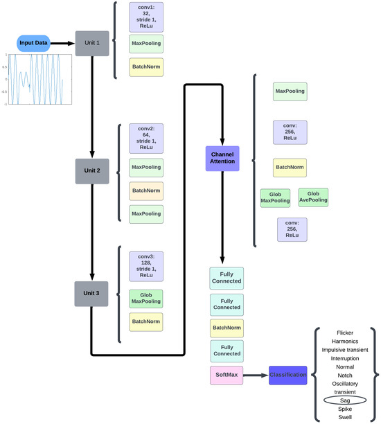
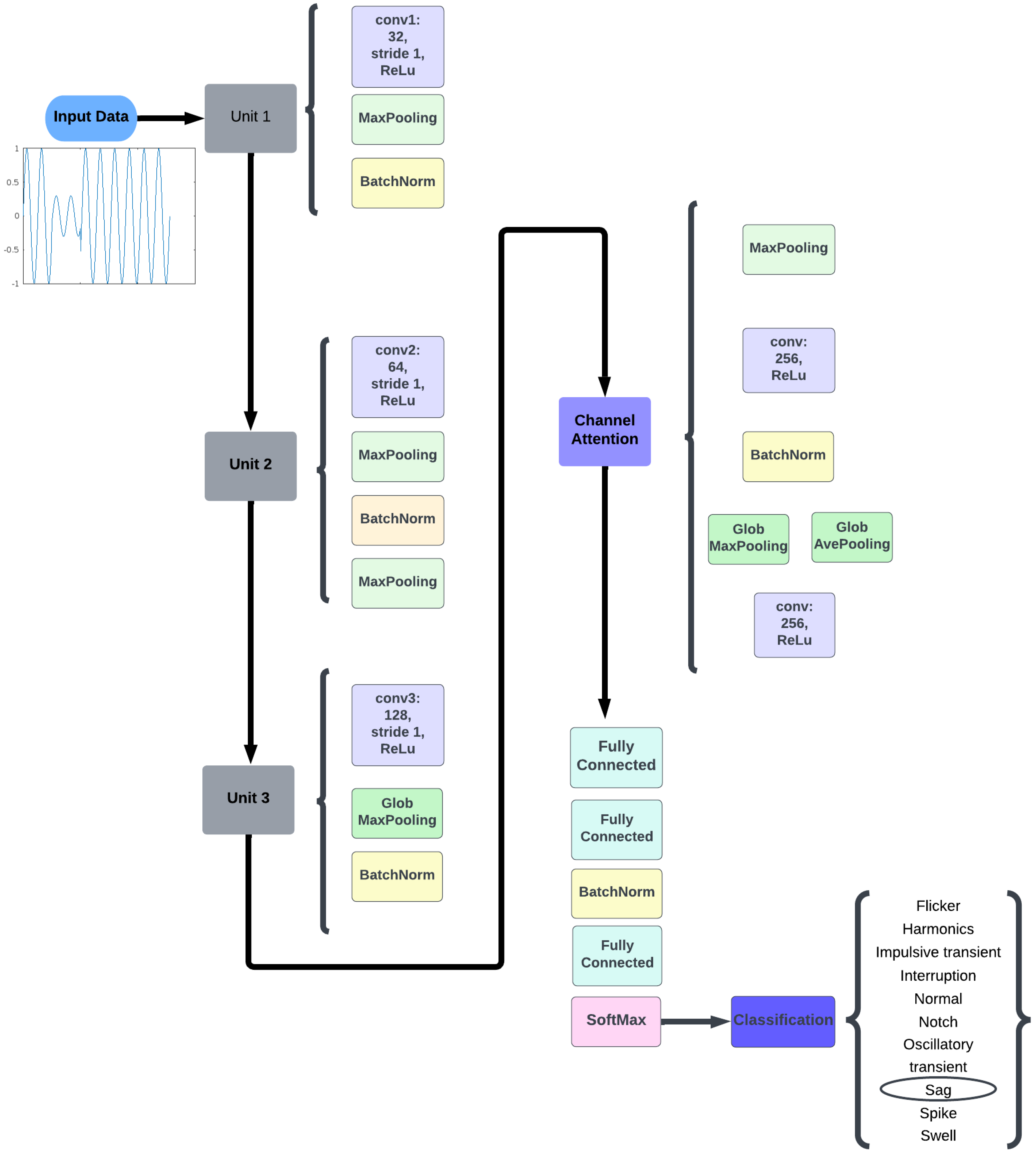
Figure 2. Proposed CNN structure.

Table 1. Proposed CNN architecture.

No.	Layer	Parameters	Activation
1	Convolution	Filter size = 32	Relu
2		Max pooling
3		Batch normalization
4	Convolution	Filter size = 64	Relu
5		Max pooling
6		Batch normalization
7		Max pooling
8	Convolution	Filter size = 128	Relu
9		Global Max pooling
10		Batch normalization
11	Attention layer
12	Fully connected	Size = 128	Relu
13	Fully connected	Size = 32	Relu
14		Batch normalization
15	Fully connected	Size = 16	Softmax

3.1. Convolution Layers

This study is based on the utilization of a 1-D CNN model for the classification of power quality disturbances. Specifically, a sliding window approach is employed to segment the signals for input into the 1-D CNN model. This strategy allows for the extraction of local features from the signal data, enabling the model to effectively capture temporal patterns and variations of essential features for accurate classification. Assuming that the sliding window iterates one element at a time (i.e., with a stride of 1), the operation can be executed based on the following definitions:

$${(I\ast K)}_i=\sum _{u=1}^{s}I(i+u-1)K\left(u\right)$$

(1)

$${(I\ast K)}_i=\sum _{u=1}^{s}I(i-u-1)K\left(u\right)$$

(2)

where I is the input of length n and K is the sliding window of length s.

By incorporating the sliding window approach in conjunction with the 1-D CNN architecture, we aim to enhance the model’s ability to analyze and classify power quality disturbances with a focus on temporal dynamics. This approach contributes significantly to the robustness and efficiency of our classification methodology, allowing for a more nuanced understanding of the complex waveforms associated with various PQ issues. The convolutional layers are utilized to perform convolutional operations on the input data sequence, effectively extracting meaningful features essential for subsequent processing. The proposed model employs multiple convolutional layers with varying kernel sizes, each dedicated to detecting specific patterns or features within the input sequence. With a stride of 1, each filter moves horizontally and vertically across the input data, advancing one position at a time. This configuration enables the convolutional layers to apply filters through element-wise multiplications and summations, leading to the generation of feature maps. A detailed overview of each convolutional layer, alongside its corresponding kernel sizes, is presented in Figure 2 and Table 1.

The ReLU activation function is utilized by introducing non-linearity into the proposed model. It is defined mathematically as:

$$f\left(x\right)=max(0,x)$$

(3)

thus, when x is positive, the output is x. On the other hand, when x is negative, the output is 0. Introducing non-linearity into our model enables the CNN to learn complex patterns. Moreover, ReLU maintains a gradient of 1 for positive inputs, facilitating faster learning in the deep network.

3.2. Max Pooling

Max pooling is a down-sampling technique used in the CNNs to reduce the spatial dimensions of feature maps while retaining the most important information. The operation involves sliding a kernel over the input feature map and taking the maximum value within that window. Thus, max pooling helps decrease computational load and mitigate overfitting. Also, it provides a degree of invariance to small translations in the input data, allowing the model to focus on dominant features regardless of their exact position.

3.3. Batch Normalization

Batch normalization is used here to improve the training speed and stability of the proposed CNN. It normalizes the outputs of the previous layer by adjusting and scaling them based on the mean and variance computed from mini-batches during training. Thus, for each mini-batch, it calculates the mean and variance of the layer’s outputs. Then, it normalizes the outputs using the following equation:

$$\widehat{x}={\displaystyle \frac{\overline{x}-\mu }{\sqrt{{\sigma }^2+ϵ}}}$$

(4)

where $\mu$ is the is the mean, ${\sigma }^2$ is the variance, and $ϵ$ is a small constant added for numerical stability. The final step in batch normalization includes scaling and shifting the normalized output using learnable parameters $\gamma$ and $\beta$:

$$y=\gamma \widehat{x}+\beta$$

(5)

3.4. Channel Attention Mechanism Unit

An integrated attention model emphasizes significant features by assigning weights based on their relevance to the classification task. This adaptive prioritization enables the model to focus on specific aspects of the input data, thereby enhancing classification accuracy. In this work, a channel attention mechanism is utilized, particularly suited for PQD data, which is represented as time-series signals. Given that the temporal characteristics of these signals are crucial, the proposed approach concentrates on specific time intervals to effectively capture relevant patterns associated with various types of disturbances. Thus, the proposed model can better discern subtle variations in the data, leading to more accurate and reliable classifications of PQDs. The channel attention mechanism typically consists of two main steps: squeeze and excitation. The squeeze operation aims to aggregate spatial information into a channel descriptor. This is accomplished using global average pooling, which summarizes the feature maps across spatial dimensions (height and width).

$$z_c={\displaystyle \frac{1}{HW}}\sum _{i=1}^H\sum _{j=1}^W{F}_c(i,j)$$

(6)

where $z_c$ is the channel descriptor for channel c, H and W are the height and width of the feature map, and $F_c(I,j)$ represents the value at position $(i,j)$ in channel c.

The excitation operation generates attention weights for each channel based on the channel descriptors obtained from the squeeze step.

3.5. The Fully Connected Layer

The fully connected layer 1 is a layer in the CNN architecture that follows the convolutional layers. It establishes a fully connected network structure by connecting every neuron from the previous layer to the current layer. The input size of fully connected layer 1 is 128, which is typically a flattened vector representing the output of the previous layer. Fully connected layer 1 takes the flattened vector as the input and performs matrix multiplication. Each neuron in fully connected layer 1 receives inputs from all of the neurons in the previous layer. Following the matrix multiplication, a bias term may be added to each neuron. This bias term enables the network to shift its decision boundary, allowing for more flexibility in the model’s predictions. The resulting values are then passed through an activation function, commonly ReLU (rectified linear unit), to introduce non-linearity and enhance the model’s representational capabilities. Furthermore, the input size of fully connected layer 2 is 32 neurons, indicating that it receives a 32-dimensional input from the previous layer. Similarly, fully connected layer 3 has an input size of 16 neurons, meaning it processes a 16-dimensional input. The specific sizes of these layers may vary depending on the network architecture and the requirements of the task at hand.

3.6. The Softmax Layer

The softmax layer is a common choice for the final layer in a classification neural network. It takes the output from the previous layer, typically a fully connected layer, and produces probabilities for each class in a multi-class classification problem. The softmax function operates on each element $x_i$ of the input vector and computes the following:

$$softmax\left(x_i\right)={\displaystyle \frac{exp\left(x_i\right)}{{\sum }_{j=1}^{N}exp\left(x_j\right)}}$$

(7)

Hence, the softmax function exponentiates each element, divides it by the sum of exponentiated values across all elements, and normalizes the result to ensure that the probabilities sum up to 1.

3.7. The Classification Layer

The classification layer is the final layer in a neural network model designed for classification tasks. Its purpose is to map the extracted features from the preceding layers of the network to the corresponding class labels.

The output of the classification layer is a vector of probabilities, where each element represents the probability of the corresponding class. The class with the highest probability is often selected as the predicted class for the input.

3.8. Data Generation

Generating synthetic PQDs includes generating voltage and current waveforms with different types of disturbance [7,21,22]. The disturbances are introduced by manipulating the waveform parameters based on established models and algorithms. Moreover, the generated PQDs are labeled and annotated according to their type and severity. This annotation process ensures that the generated dataset contains accurate labels for the different types of disturbances, which are essential for training and evaluating deep learning models.

Two datasets were generated using [7]. The first dataset consists of PQ signals with random Gaussian noise, where the signal-to-noise ratio (SNR) ranges between 20 and 50 dB. The second dataset is generated without any noise. Each dataset contains a total of 50,000 signals, with 5000 signals being dedicated to each disturbance type. The disturbance types included in the datasets are as follows: normal, flicker, harmonics, oscillatory transient, impulsive transient, interruption, notch, sag, spike, and swell.

The datasets aim to provide a diverse representation of PQDs encountered in real-world scenarios. By including different disturbance types and generating datasets with and without noise, the authors enable the evaluation and comparison of various algorithms and techniques for PQ analysis and classification tasks. Collectively, these datasets facilitate a thorough evaluation of the proposed approach across varied contexts and conditions. To maintain analytical consistency, each dataset is segmented into training (60%), validation (20%), and test (20%) subsets. This partitioning allows for effective model training, unbiased performance assessment during the validation phase, and a final evaluation of the model’s generalization capabilities on unseen data. Such a rigorous approach not only strengthens the validity of the findings but also facilitates meaningful comparisons with existing methodologies, ultimately contributing to the advancement of power quality disturbance classification techniques.

Data augmentation is utilized to expand and diversify the training dataset, enhancing the performance and generalization capabilities of the proposed model. By altering the temporal characteristics of PQD signals through the addition of noise to the time domain data, the proposed model can effectively learn to identify and generalize patterns across varying noise levels and temporal scales, improving its robustness and accuracy in classifying power quality disturbances.

3.9. Experimental Setup and Network Training

The experiments were conducted using a robust hardware setup that includes an AMD CPU, Intel processors, and Nvidia Tesla T4 GPUs. This configuration boasts a total of 24 cores and an impressive 384 GB of combined memory, providing ample resources for intensive computational tasks. The experiments were executed using MATLAB software, ensuring access to the latest features and optimizations for data analysis and algorithm development.

Bayesian optimization, a sophisticated approach to hyperparameter tuning, is systematically employed across all models in this study. The optimization procedure is based on Bayes’ theorem [23], such that for a model Z and observation Y:

$$P\left(z\right|y)=(P\left(Y\right|Z\left)P\right(z\left)\right)/P\left(z\right)$$

(8)

where $P\left(Z\right|Y)$ is the posterior probability of Z given Y, $P\left(Y\right|Z)$ is the likelihood of Y given Z, $P\left(Z\right)$ is the prior probability of Z, and $P\left(Z\right)$ is the marginal probability of Z. This advanced technique leverages probabilistic models to intelligently navigate the complex hyperparameter space, striking an optimal balance between the exploration of new parameter combinations and the exploitation of known high-performing regions. By consistently applying this process to each model, including the proposed method and all comparison models, the aim is to ensure a fair, rigorous, and unbiased evaluation framework. This methodical approach not only maximizes the potential of each model to achieve its peak performance on the given datasets but also mitigates the risk of performance disparities arising from inconsistent tuning practices. Furthermore, this standardized tuning process enhances the reproducibility of the results, provides a solid foundation for future research in this domain, and ensures that any performance differences observed between models are more likely to be inherent to the models themselves rather than artifacts of the tuning process.

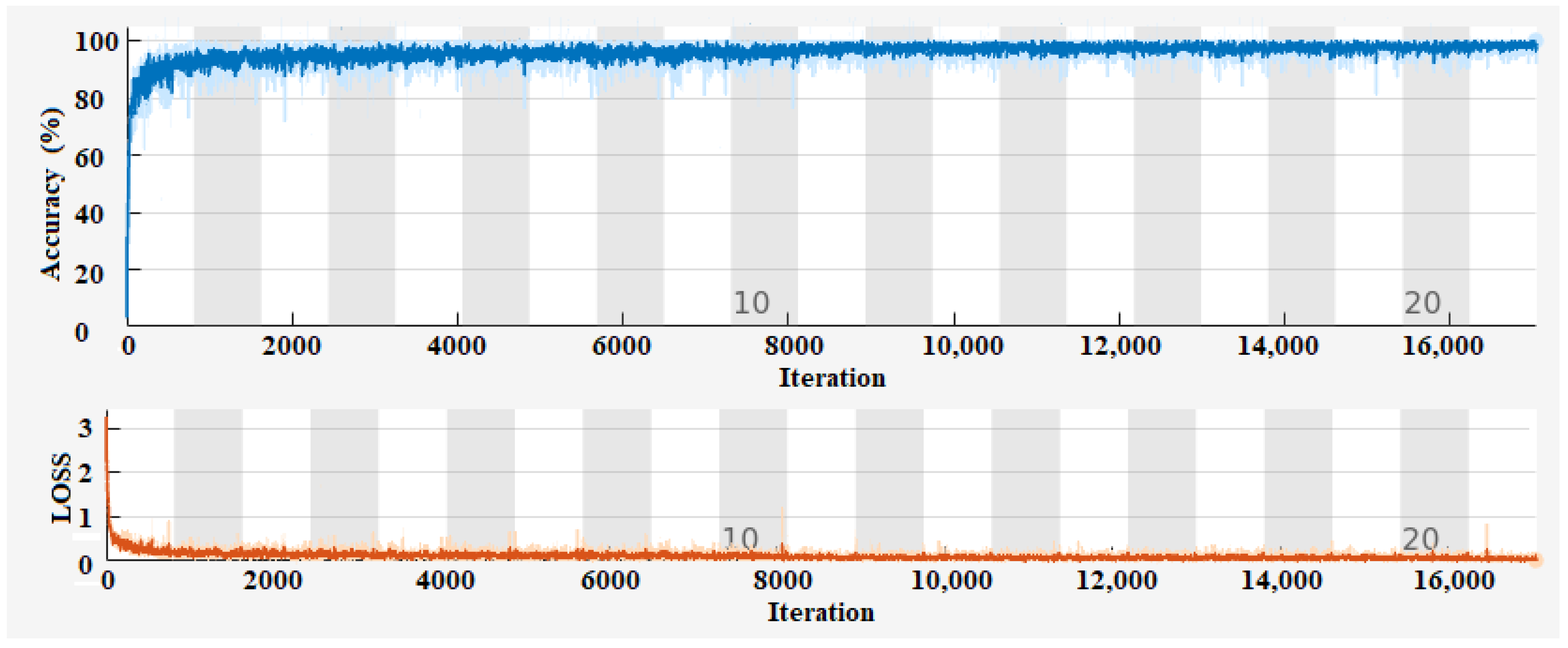
Thus, the CNN networks are trained using the Adam optimizer with specific training options, including a maximum of 21 epochs, a mini-batch size of 64, a piecewise learning rate schedule with a drop factor of 0.5, a drop period of 10 epochs, an initial learning rate of 0.01, a gradient threshold of 1, and automatic execution environment selection. Training progress is monitored and visualized using training progress plots. Figure 3 shows the training progress of the proposed CNN. The graph demonstrates the performance improvement of the CNN model over multiple epochs. As the number of epochs increases, the accuracy of the model steadily increases. This indicates that the model is learning and making better predictions as it receives more training data and updates its internal parameters.

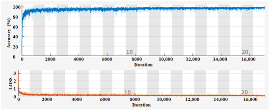
Figure 3. Training progress of the proposed CNN.

Moreover, the RNN networks are trained using the “Adam” optimizer with the maximum number of training epochs being set to 60. The number of samples in each mini-batch is set to 64, and a piecewise learning rate schedule is employed. The drop factor is set to 0.5 with a drop period of 10 epochs, an initial learning rate of 0.01, and a gradient threshold of 1. The “Execution Environment” is set to “auto”, enabling the code to automatically utilize available hardware resources.

4. Results and Discussion

The performance of the proposed network undergoes a comprehensive evaluation, pitting it against a diverse array of state-of-the-art architectures. This evaluation encompasses both CNN models and RNN models, providing a broad spectrum of comparison points. Among the CNN models, the evaluation includes a CNN architecture detailed in [7] and ResNet50. This comparison allows for a nuanced understanding of how the proposed network performs against both simpler and more complex CNN architectures. The evaluation extends to RNN models as well, incorporating BiLSTM and GRU models. These RNN variants are adept at capturing temporal dependencies in sequential data, offering a different perspective on the problem compared with CNN-based approaches. This multi-faceted comparison strategy ensures a thorough assessment of the proposed network’s capabilities across various architectural paradigms. It not only benchmarks the network against established models but also provides insights into its relative strengths and potential areas for improvement across different types of neural network architectures.

Quantitative Evaluation

Table 2, Table 3, Table 4, Table 5 and Table 6 present the confusion matrices for the proposed CNN, along with those of the compared state-of-the-art methods on datasets without noise. Additionally, Table 7, Table 8, Table 9, Table 10 and Table 11 display the confusion matrices for the proposed CNN and the state-of-the-art methods on datasets with noise.

Table 2. Confusion matrix of the training data using the proposed CNN architecture, without noise.

True values	Flicker	1747	0	0	2	0	0	0	0	0	1
	Harmonics	0	1750	0	0	0	0	0	0	0	0
	Impulsive transient	0	0	1740	3	2	1	1	3	0	0
	Interruption	0	0	3	1744	0	0	3	1	0	0
	Normal	0	0	0	0	1748	0	0	0	0	0
	Notch	0	0	5	0	0	1745	0	0	0	0
	Oscillatory transient	0	0	2	2	0	4	1744	1	0	1
	Sag	0	0	0	0	0	0	0	1744	5	1
	Spike	0	0	0	0	0	0	0	0	1745	0
	Swell	0	0	0	0	0	0	2	1	0	1747
Predicted values

Table 3. Confusion matrix of the training data using the CNN architecture in [7], without noise.

True values	Flicker	1734	0	2	0	3	0	4	5	0	1
	Harmonics	0	1750	0	0	0	0	0	0	0	0
	Impulsive transient	0	0	1708	0	24	0	18	0	0	0
	Interruption	0	0	23	1703	19	0	0	5	0	0
	Normal	0	0	0	0	1750	0	0	0	0	0
	Notch	0	0	6	0	55	1688	0	0	0	1
	Oscillatory transient	0	0	17	0	11	0	1715	0	0	7
	Sag	0	0	30	12	13	0	0	1695	0	0
	Spike	0	0	5	0	45	1	0	1	1698	0
	Swell	0	0	5	0	12	0	8	0	0	1725
Predicted values

Table 4. Confusion matrix of the training data using the ResNet50 architecture, without noise.

True values	Flicker	1740	0	1	0	2	0	2	3	0	1
	Harmonics	0	1750	0	0	0	0	0	0	0	0
	Impulsive transient	0	0	1728	0	10	0	12	0	0	0
	Interruption	0	0	10	1725	8	0	0	7	0	0
	Normal	0	0	0	0	1750	0	0	0	0	0
	Notch	0	0	3	0	30	1715	0	0	0	2
	Oscillatory transient	0	0	8	0	5	0	1735	0	0	2
	Sag	0	0	15	5	6	0	0	1724	0	0
	Spike	0	0	3	0	20	0	0	0	1728	0
	Swell	0	0	1	0	5	0	3	0	0	1740
Predicted values

Table 5. Confusion matrix of the training data using BiLSTM architecture, without noise.

True values	Flicker	1640	0	8	2	0	38	0	2	26	4
	Harmonics	0	1748	0	0	0	0	0	0	0	0
	Impulsive transient	2	0	1556	22	4	2	0	0	0	0
	Interruption	0	0	7	1658	2	3	0	46	0	0
	Normal	0	0	0	0	1740	0	0	0	0	0
	Notch	23	0	8	5	2	1551	6	0	9	0
	Oscillatory transient	18	0	4	0	1	33	1291	0	10	9
	Sag	0	0	3	12	1	1	0	1326	0	0
	Spike	12	0	0	0	0	0	13	0	1668	0
	Swell	0	0	2	0	0	0	15	0	0	1613
Predicted values

Table 6. Confusion matrix of the training data using GRU architecture, without noise.

True values	Flicker	1660	0	6	1	0	30	0	1	20	2
	Harmonics	0	1749	0	0	1	0	0	0	0	0
	Impulsive transient	1	0	1580	18	2	1	0	0	0	0
	Interruption	0	0	5	1670	1	2	0	38	0	0
	Normal	0	0	0	0	1745	0	0	0	0	0
	Notch	18	0	6	3	1	1570	4	0	6	0
	Oscillatory transient	14	0	2	0	0	25	1320	0	8	7
	Sag	0	0	2	9	0	0	0	1332	0	0
	Spike	9	0	0	0	0	0	10	0	1674	0
	Swell	0	0	1	0	0	0	12	0	0	1617
Predicted values

Table 7. Confusion matrix of the training data using the proposed CNN architecture, with noise.

True values	Flicker	1749	0	0	0	0	0	0	1	0	0
	Harmonics	0	1750	0	0	0	0	0	0	0	0
	Impulsive transient	0	0	1750	0	0	0	0	0	0	0
	Interruption	0	0	0	1744	0	3	0	3	0	0
	Normal	0	0	0	0	1750	0	0	0	0	0
	Notch	0	0	0	5	0	1745	0	0	0	0
	Oscillatory transient	1	0	0	0	0	0	1745	3	1	0
	Sag	0	0	0	1	0	2	4	1743	0	0
	Spike	0	0	0	0	0	0	1	0	1749	0
	Swell	0	0	0	0	0	0	0	0	0	1750
Predicted values

Table 8. Confusion matrix of the training data using the CNN architecture in [7], with noise.

True values	Flicker	1719	0	0	0	0	0	0	3	0	0
	Harmonics	0	1747	0	0	0	0	0	0	0	0
	Impulsive transient	0	0	1730	0	0	0	20	0	0	0
	Interruption	0	0	0	1748	0	0	0	2	0	0
	Normal	0	0	0	0	1750	0	0	0	0	0
	Notch	0	0	0	3	0	1718	0	29	0	0
	Oscillatory transient	0	0	44	0	0	0	1706	0	0	0
	Sag	0	0	0	1	0	0	0	1749	0	0
	Spike	0	0	0	0	0	1	0	0	1749	0
	Swell	0	0	0	0	0	0	0	0	0	1750
Predicted values

Table 9. Confusion matrix of the training data using the ResNet50 architecture, with noise.

True values	Flicker	1722	0	0	0	0	0	0	1	0	0
	Harmonics	0	1748	0	0	0	0	0	0	0	0
	Impulsive transient	0	0	1738	0	0	0	12	0	0	0
	Interruption	0	0	0	1749	0	0	0	1	0	0
	Normal	0	0	0	0	1750	0	0	0	0	0
	Notch	0	0	0	1	0	1730	0	19	0	0
	Oscillatory transient	0	0	30	0	0	0	1720	0	0	0
	Sag	0	0	0	0	0	0	0	1750	0	0
	Spike	0	0	0	0	0	0	0	0	1750	0
	Swell	0	0	0	0	0	0	0	0	0	1750
Predicted values

Table 10. Confusion matrix of the training data using BiLSTM architecture, with noise.

True values	Flicker	1710	0	2	0	0	2	0	0	5	0
	Harmonics	0	1745	0	11	2	15	0	5	0	2
	Impulsive transient	0	0	1675	2	0	2	0	0	15	0
	Interruption	3	0	0	1674	3	6	2	3	0	10
	Normal	0	1	5	0	1678	0	0	12	0	0
	Notch	14	0	4	2	0	1417	5	0	4	5
	Oscillatory transient	7	2	3	0	4	12	1654	0	2	0
	Sag	0	0	1	1	3	0	0	1456	0	1
	Spike	6	2	0	0	0	3	16	0	1670	0
	Swell	0	0	0	0	1	0	1	0	0	1731
Predicted values

Table 11. Confusion matrix of the training data using GRU architecture, with noise.

True values	Flicker	1715	0	1	0	0	1	0	0	3	0
	Harmonics	0	1748	0	8	1	10	0	3	0	1
	Impulsive transient	0	0	1685	1	0	1	0	0	10	0
	Interruption	2	0	0	1680	2	4	1	2	0	7
	Normal	0	0	3	0	1685	0	0	8	0	0
	Notch	10	0	2	1	0	1430	3	0	2	3
	Oscillatory transient	5	1	2	0	2	8	1665	0	1	0
	Sag	0	0	0	0	2	0	0	1462	0	0
	Spike	4	1	0	0	0	2	12	0	1678	0
	Swell	0	0	0	0	0	0	0	0	0	1733
Predicted values

The performance of the proposed method, as evidenced by the confusion matrix, demonstrates a significant advancement over existing state-of-the-art techniques. This detailed analysis highlights the classification results and also showcases the model’s ability to accurately predict various classes of PQDs. By systematically comparing the confusion matrices of the proposed method with those of leading approaches, the proposed method can effectively evaluate key performance metrics such as precision, recall, and overall accuracy for each class. The results reveal that the introduced method consistently outperforms its competitors, achieving higher precision and recall rates across multiple PQD classes. This indicates that the proposed approach enhances classification accuracy and also improves the model’s reliability in distinguishing between different categories of PQDs.

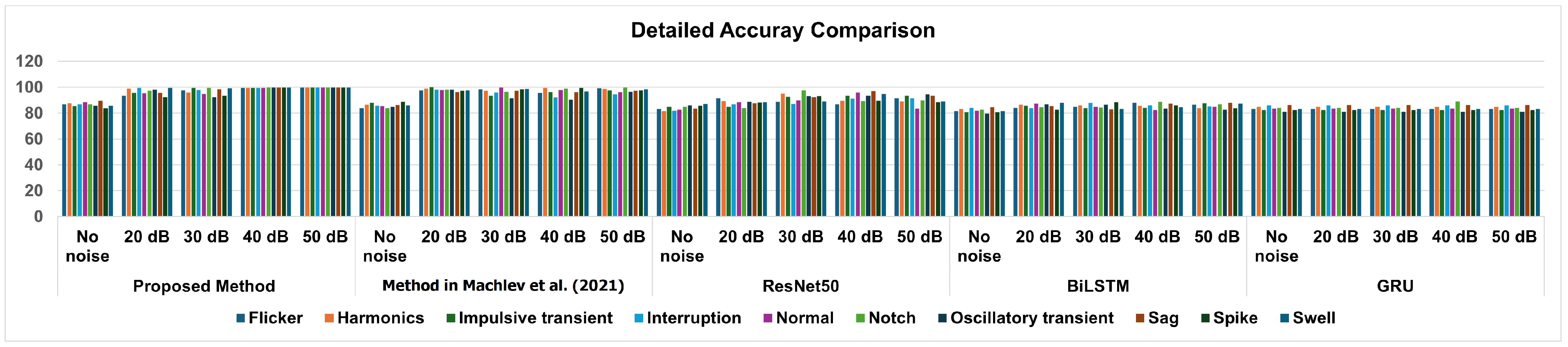
Table 12, Table 13, Table 14, Table 15 and Table 16 provide detailed accuracy values for the proposed approach and the state-of-the-art methods. The accuracy values presented in these tables offer a comprehensive comparison of the proposed method against its alternatives. The proposed approach demonstrates superior performance across all evaluated classes, particularly evident in the accuracy metric, where it consistently outperforms the competing methods. This indicates a stronger ability to correctly identify and classify instances across various categories.

Table 12. Detailed accuracy of the proposed method.

	No Noise	20 dB	30 dB	40 dB	50 dB
Flicker	86.633	93.441	97.601	99.541	99.521
Harmonics	87.602	98.992	95.712	99.512	99.522
Impulsive transient	85.292	93.473	99.503	99.493	99.523
Interruption	86.626	99.496	97.932	99.614	99.524
Normal	88.625	95.195	94.605	99.825	99.525
Notch	86.637	97.436	99.298	99.466	99.526
Oscillatory transient	85.663	98.197	92.507	99.517	99.527
Sag	89.659	95.498	98.392	99.518	99.628
Spike	83.648	92.448	93.523	99.519	99.459
Swell	85.624	99.507	99.241	99.52	99.530

Table 13. Detailed accuracy of the CNN method in [7].

	No Noise	20 dB	30 dB	40 dB	50 dB
Flicker	83.801	97.514	98.245	95.594	99.191
Harmonics	86.419	98.982	97.242	99.301	98.604
Impulsive transient	87.922	99.851	93.547	96.357	97.447
Interruption	85.724	98.170	95.718	92.124	94.458
Normal	85.515	97.723	99.656	97.841	95.974
Notch	83.894	98.181	96.479	98.978	99.712
Oscillatory transient	84.911	98.149	91.247	90.374	96.514
Sag	86.256	96.375	97.392	95.981	97.325
Spike	88.742	97.244	98.283	99.27	97.647
Swell	85.901	97.470	98.541	96.781	98.362

Table 14. Detailed accuracy of the ResNet50 method.

	No Noise	20 dB	30 dB	40 dB	50 dB
Flicker	82.991	91.225	88.636	86.412	91.391
Harmonics	81.147	89.282	95.122	89.751	89.856
Impulsive transient	84.472	84.915	92.961	93.541	93.124
Interruption	81.635	86.737	87.018	91.124	91.516
Normal	82.157	88.523	89.756	95.641	83.474
Notch	84.871	83.781	97.479	89.278	89.812
Oscillatory transient	85.571	88.349	93.247	93.374	94.468
Sag	83.754	87.172	92.224	97.181	93.711
Spike	85.465	88.244	93.083	89.473	88.372
Swell	86.635	88.574	89.814	94.124	89.461

Table 15. Detailed accuracy of the BiLSTM method.

	No Noise	20 dB	30 dB	40 dB	50 dB
Flicker	81.425	84.123	84.89	87.890	86.345
Harmonics	83.124	86.456	86.001	85.678	83.890
Impulsive transient	80.750	85.678	83.789	84.234	87.456
Interruption	84.250	83.901	87.654	86.012	85.234
Normal	81.741	87.234	85.012	82.345	84.89
Notch	82.499	84.567	84.321	88.789	86.789
Oscillatory transient	79.374	86.789	86.543	83.456	82.567
Sag	84.578	85.345	82.789	87.123	88.012
Spike	80.759	82.456	88.456	85.89	83.678
Swell	81.574	88.123	83.210	84.678	87.210

Table 16. Detailed accuracy of the GRU method.

	No Noise	20 dB	30 dB	40 dB	50 dB
Flicker	83.054	85.805	86.588	89.648	88.072
Harmonics	84.786	88.185	87.721	87.392	85.568
Impulsive transient	82.365	87.392	85.465	85.919	89.205
Interruption	85.935	85.588	89.407	87.732	86.939
Normal	83.376	88.979	86.712	83.992	86.588
Notch	84.149	86.258	86.007	90.565	88.525
Oscillatory transient	80.961	88.525	88.274	85.125	84.218
Sag	86.270	87.052	84.445	88.865	89.772
Spike	82.374	84.105	90.225	87.608	85.352
Swell	83.205	89.885	84.874	86.372	88.954

Furthermore, the overall results illustrate that the proposed method effectively minimizes false positives and false negatives compared with both competing models, highlighting its robustness and reliability in classification tasks. Overall, these results underscore the efficacy of the proposed method in delivering enhanced accuracy and performance relative to existing state-of-the-art techniques.

Figure 4 presents a comprehensive bar chart illustrating the detailed accuracy of the proposed approach and the state-of-the-art methods. This visual representation allows for an easy comparison of the performance metrics across these approaches, highlighting the strengths and weaknesses of each model in terms of classification accuracy. By examining the bar chart, viewers can quickly discern how the proposed method stands out in achieving superior accuracy compared with its counterparts, thereby emphasizing its effectiveness in addressing classification challenges.

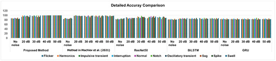
Figure 4. Detailed accuracy of the proposed method compared with the state-of-the-art methods [7].

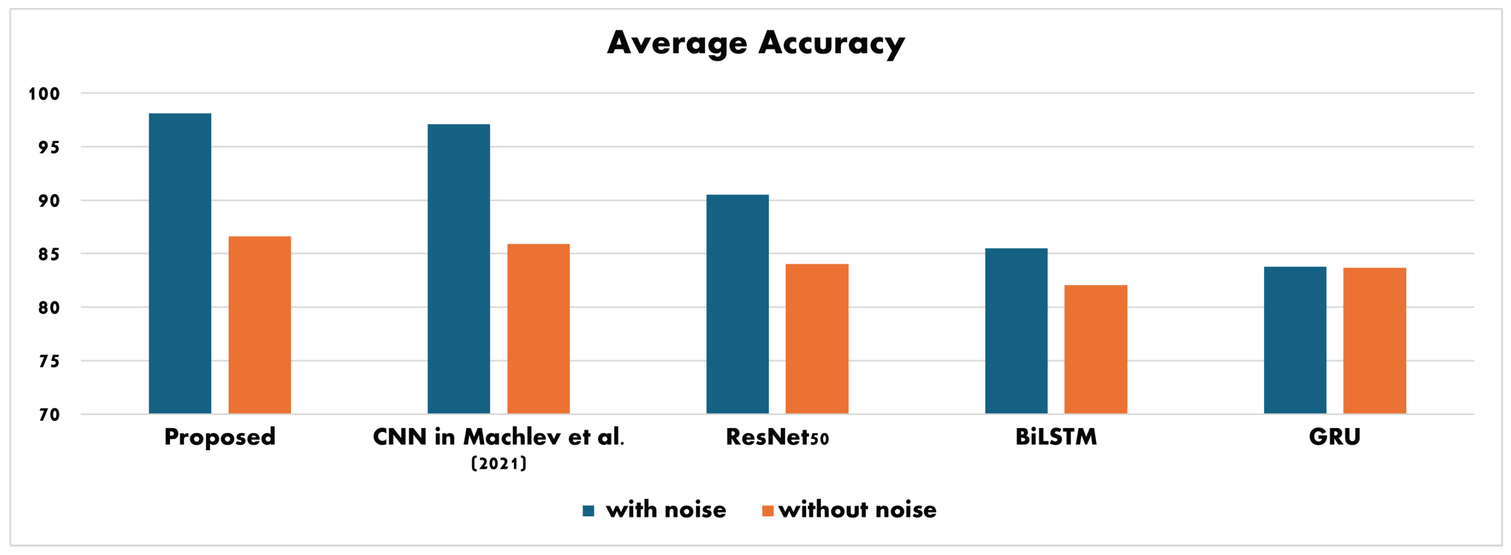
Table 17 provides a comprehensive overview of the average accuracy achieved by the proposed CNN and other state-of-the-art methods. It presents a quantitative measure of how well each method performs in accurately classifying the test data.

Table 17. Testing average accuracy comparison.

Method	With Noise	Without Noise
Proposed	98.110	86.607
CNN in [7]	97.096	85.907
ResNet50	90.505	84.027
BiLSTM	85.487	82.025
GRU	83.772	83.647

On the other hand, Figure 5 visually represents the testing accuracy levels of the proposed CNN and state-of-the-art methods. This graphical representation enables a more intuitive understanding of the performance comparison. By examining both the table and the figure, the proposed CNN performs well compared with the existing state-of-the-art methods in terms of testing accuracy.

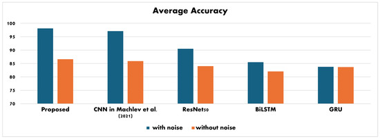
Figure 5. Testing average accuracy comparison [7].

The proposed model achieved an accuracy of up to $99.49\%$, significantly outperforming traditional methods and even some existing models. This demonstrates the effectiveness of leveraging multi-scale CNNs combined with attention mechanisms to capture complex patterns in PQ signals. The integration of attention mechanisms allows the model to focus on the most relevant features of the input data, enhancing its ability to discern subtle variations in power quality disturbances. This can lead to more reliable classifications, especially in noisy environments. By improving the accuracy and efficiency of PQ analysis, the proposed approach has significant implications for real-world applications. Enhanced classification can lead to better monitoring and maintenance of power systems, ultimately contributing to increased reliability and stability of electrical grids. Moreover, future research could explore the model’s scalability and its performance in real-time applications, where rapid and accurate classification of PQ disturbances is crucial. Additionally, investigating the interpretability of the model’s decisions could provide valuable insights into the specific features it relies on for classification, potentially leading to further improvements in PQ analysis techniques.

5. Conclusions and Future Work

This work introduces a novel deep learning approach for classifying PQDs. The method harnesses deep neural networks’ capabilities to accurately identify and categorize various PQDs, enabling effective analysis and monitoring of electrical systems. By leveraging deep learning algorithms, particularly CNNs enhanced with a channel attention mechanism, the proposed method has demonstrated enhanced classification accuracy for PQDs. The model shows proficiency in learning intricate patterns and features from PQ signals, leading to robust and reliable classification performance. This advancement not only improves disturbance detection precision but also enhances overall electrical system efficiency and stability, laying the groundwork for more effective PQ management and mitigation strategies.

The outcomes from the deep learning approach are promising, highlighting its potential to elevate PQ analysis and monitoring systems. Undetected or misdiagnosed PQ issues can result in operational disruptions, equipment failures, increased downtime, and safety risks. Inaccurate identification also hampers targeted mitigation strategies, undermining PQ quality and potentially causing economic losses.

The proposed deep learning methodology opens the door to further exploration in PQ analysis. Future investigations will involve conducting ablation experiments to assess the specific impact of the channel attention mechanism within the deep learning model. These experiments will provide insights into the mechanism’s contribution to classification accuracy, further refining the model and potentially enhancing its performance. Additionally, ongoing research efforts will focus on continuously improving deep learning architectures, exploring sophisticated ensemble methods, and integrating additional relevant features to push the boundaries of classification performance. Moreover, modifying the structure and training algorithm of the developed CNN will be a priority. This research has the potential to revolutionize power system management by advancing our understanding and capabilities in PQ analysis. It could lead to a more reliable and resilient electrical infrastructure that can meet the evolving demands of modern society.

References

- Khetarpal, P.; Tripathi, M.M. A critical and comprehensive review on power quality disturbance detection and classification. Sustain. Comput. Inform. Syst. 2020, 28, 100417. [Google Scholar] [CrossRef]
- Samanta, I.S.; Panda, S.; Rout, P.K.; Bajaj, M.; Piecha, M.; Blazek, V.; Prokop, L. A Comprehensive Review of Deep-Learning Applications to Power Quality Analysis. Energies 2023, 16, 4406. [Google Scholar] [CrossRef]
- Qader, M.R. A Method for Analytical Voltage Sags Prediction in Complex Power Network. Recent Adv. Electr. Electron. Eng. 2018, 11, 303–309. [Google Scholar] [CrossRef]
- Thentral, T.T.; Palanisamy, R.; Usha, S.; Bajaj, M.; Zawbaa, H.M.; Kamel, S. Analysis of Power Quality issues of different types of household applications. Energy Rep. 2022, 8, 5370–5386. [Google Scholar] [CrossRef]
- Sharma, A.; Rajpurohit, B.S.; Singh, S. A review on economics of power quality: Impact, assessment and mitigation. Renew. Sustain. Energy Rev. 2018, 88, 363–372. [Google Scholar] [CrossRef]
- Iturrino Garcia, C.A.; Bindi, M.; Corti, F.; Luchetta, A.; Grasso, F.; Paolucci, L.; Piccirilli, M.C.; Aizenberg, I. Power Quality Analysis Based on Machine Learning Methods for Low-Voltage Electrical Distribution Lines. Energies 2023, 16, 3627. [Google Scholar] [CrossRef]
- Machlev, R.; Chachkes, A.; Belikov, J.; Beck, Y.; Levron, Y. Open source dataset generator for power quality disturbances with deep-learning reference classifiers. Electr. Power Syst. Res. 2021, 195, 107152. [Google Scholar] [CrossRef]
- Albalooshi, F.A.; Asari, V.K. Fast and robust object region segmentation with self-organized lattice Boltzmann based active contour method. J. Electron. Imaging 2024, 33, 043050. [Google Scholar] [CrossRef]
- Liu, Y.; Shen, L.; Zhu, X.; Xie, Y.; He, S. Spectral Data-Driven Prediction of Soil Properties Using LSTM-CNN-Attention Model. Appl. Sci. 2024, 14, 11687. [Google Scholar] [CrossRef]
- Albalooshi, F.A. Novel Approach in Vegetation Detection Using Multi-Scale Convolutional Neural Network. Appl. Sci. 2024, 14, 10287. [Google Scholar] [CrossRef]
- Wang, S.; Chen, H. A novel deep learning method for the classification of power quality disturbances using deep convolutional neural network. Appl. Energy 2019, 235, 1126–1140. [Google Scholar] [CrossRef]
- Jamlus, N.U.I.A.; Shahbudin, S.; Kassim, M. Power Quality Disturbances Classification Analysis Using Residual Neural Network. In Proceedings of the 2022 IEEE 18th International Colloquium on Signal Processing & Applications (CSPA), Selangor, Malaysia, 12 May 2022; pp. 442–447. [Google Scholar] [CrossRef]
- Bravo-Rodríguez, J.C.; Torres, F.J.; Borrás, M.D. Hybrid Machine Learning Models for Classifying Power Quality Disturbances: A Comparative Study. Energies 2020, 13, 2761. [Google Scholar] [CrossRef]
- Dekhandji, F.Z.; Recioui, A.; Ladada, A.; Moulay Brahim, T.S. Detection and Classification of Power Quality Disturbances Using LSTM. Eng. Proc. 2023, 29, 2. [Google Scholar] [CrossRef]
- Gunawan, T.S.; Husodo, B.Y.; Ihsanto, E.; Ramli, K. Power Quality Disturbance Classification Using Deep BiLSTM Architectures with Exponentially Decayed Number of Nodes in the Hidden Layers. In Recent Trends in Mechatronics Towards Industry 4.0; Nasir, A.F.A., Ibrahim, A.N., Ishak, I., Mat Yahya, N., Zakaria, M.A., Abdul Majeed, A.P.P., Eds.; Springer: Singapore, 2022; pp. 725–736. [Google Scholar]
- Yiğit, E.; Özkaya, U.; Öztürk, Ş.; Singh, D.; Gritli, H. Automatic detection of power quality disturbance using convolutional neural network structure with gated recurrent unit. Mob. Inf. Syst. 2021, 2021, 7917500. [Google Scholar] [CrossRef]
- Khetarpal, P.; Nagpal, N.; Al-Numay, M.S.; Siano, P.; Arya, Y.; Kassarwani, N. Power quality disturbances detection and classification based on deep convolution auto-encoder networks. IEEE Access 2023, 11, 46026–46038. [Google Scholar] [CrossRef]
- Topaloglu, I. Deep learning based a new approach for power quality disturbances classification in power transmission system. J. Electr. Eng. Technol. 2023, 18, 77–88. [Google Scholar] [CrossRef]
- Beniwal, R.K.; Saini, M.K.; Nayyar, A.; Qureshi, B.; Aggarwal, A. A critical analysis of methodologies for detection and classification of power quality events in smart grid. IEEE Access 2021, 9, 83507–83534. [Google Scholar] [CrossRef]
- Ramalingappa, L.; Manjunatha, A. Power quality event classification using complex wavelets phasor models and customized convolution neural network. Int. J. Electr. Comput. Eng. (IJECE) 2022, 12, 22–31. [Google Scholar] [CrossRef]
- Khokhar, S.; Mohd Zin, A.A.; Memon, A.P.; Mokhtar, A.S. A new optimal feature selection algorithm for classification of power quality disturbances using discrete wavelet transform and probabilistic neural network. Measurement 2017, 95, 246–259. [Google Scholar] [CrossRef]
- IEEE 1159-1995; IEEE Recommended Practice for Monitoring Electric Power Quality. IEEE: Piscataway, NJ, USA, 1995.
- Herrle, S.R.; Corbett, E.C., Jr.; Fagan, M.J.; Moore, C.G.; Elnicki, D.M. Bayes’ theorem and the physical examination: Probability assessment and diagnostic decision making. Acad. Med. 2011, 86, 618–627. [Google Scholar] [CrossRef] [PubMed]
Disclaimer/Publisher’s Note: The statements, opinions and data contained in all publications are solely those of the individual author(s) and contributor(s) and not of MDPI and/or the editor(s). MDPI and/or the editor(s) disclaim responsibility for any injury to people or property resulting from any ideas, methods, instructions or products referred to in the content. |
© 2025 by the authors. Licensee MDPI, Basel, Switzerland. This article is an open access article distributed under the terms and conditions of the Creative Commons Attribution (CC BY) license (https://creativecommons.org/licenses/by/4.0/).