Short-Medium-Term Solar Irradiance Forecasting with a CEEMDAN-CNN-ATT-LSTM Hybrid Model Using Meteorological Data

Abstract

In recent years, the adverse effects of climate change have increased rapidly worldwide, driving countries to transition to clean energy sources such as solar and wind. However, these energies face challenges such as cloud cover, precipitation, wind speed, and temperature, which introduce variability and intermittency in power generation, making integration into the interconnected grid difficult. To achieve this, we present a novel hybrid deep learning model, CEEMDAN-CNN-ATT-LSTM, for short- and medium-term solar irradiance prediction. The model utilizes complete empirical ensemble modal decomposition with adaptive noise (CEEMDAN) to extract intrinsic seasonal patterns in solar irradiance. In addition, it employs a hybrid encoder-decoder framework that combines convolutional neural networks (CNN) to capture spatial relationships between variables, an attention mechanism (ATT) to identify long-term patterns, and a long short-term memory (LSTM) network to capture short-term dependencies in time series data. This model has been validated using meteorological data in a more than 2400 masl region characterized by complex climatic conditions south of Ecuador. It was able to predict irradiance at 1, 6, and 12 h horizons, with a mean absolute error (MAE) of 99.89 W/m² in winter and 110.13 W/m² in summer, outperforming the reference methods of this study. These results demonstrate that our model represents progress in contributing to the scientific community in the field of solar energy in environments with high climatic variability and its applicability in real scenarios.

1. Introduction

Global heating, the depletion of fossil resources, and international efforts to reduce carbon emissions by 2050 have driven countries to adopt renewable energies as a viable solution to generate green energy. These include solar energy, one of the most abundant and usable resources on the planet, which presents no environmental risk [1]. Efficient integration of these energies into the electrical grid and precise scheduling of available energy are fundamental for their optimal utilization [2]. Additionally, renewable energies offer sustainable and unlimited alternatives for electricity generation.

Kumar et al. [3] highlight that photovoltaic (PV) power production costs have become competitive, equaling or even surpassing those of non-renewable energy sources. As a result, the number of solar power plants is increasing considerably [4]. It is, therefore, becoming critical for utilities to have reliable and robust models that ensure the efficient operation of the power grid.

PV power generation is directly dependent on solar irradiance. Although predicting irradiance might appear to be an easy task, in reality, factors such as cloud cover, precipitation, and wind speed have a significant impact [5]. These factors introduce instability, randomness, and uncertainty into irradiance, resulting in solar power generation volatility. This variability makes it difficult to fully rely on PVs and presents a considerable challenge to the effective integration of solar generation plants into the power grid [6]. This challenge is even more complex in areas where the climate is volatile [7].

Different solar forescasting methods have been developed and experimented with over time. According to [8], solar energy prediction techniques are divided into five groups: physical methods, persistence methods, statistical methods, machine learning models, and hybrid models.

Persistence models are commonly used to compare forecasted results and evaluate model performance. According to Perez et al. [9], energy prediction models based on the persistence method are straightforward but limited. Physical methods, on the other hand, use meteorological variables defined by mathematical equations to model weather patterns, requiring significant computational resources [10]. In this context, Kocifaj and Kómar [11] proposed a unified model of irradiance patterns (UMRP) to simulate sky irradiance under various conditions. However, physical models often fail to achieve reasonable accuracy under unstable weather conditions [12].

Statistical methods rely on mathematical relationships between arbitrary and non-arbitrary variables. Examples of this method are the autoregressive integrated moving average (ARIMA) model [13], exponential smoothing [14], and multiple linear regression (MLR) [15], which efficiently model relationships between irradiance and meteorological data. Despite their utility, these models lack robustness and can produce null or incomplete values under certain conditions [16].

Machine learning (ML) approaches have become popular in the last decade, as these models can automatically learn and improve forecasting by comparing real and predicted data. Common methods include support vector machines (SVMs) [17], multi-layer perceptron (MLP) [18], extreme learning machines (ELMs) [19], and artificial neural networks (ANNs) [20]. However, the inherent volatility and randomness of irradiance makes more complex models have problems in learning from these data. Therefore, to solve this problem, hybrid models combine different architectures, such as SVMs, MLP, ELMs, and ANNs, to improve prediction efficiency and accuracy in PV power estimation.

In addition, variable decomposition techniques, such as empirical mode decomposition (EMD), ensemble empirical mode decomposition (EEMD), and wavelet decomposition (WT), are used to capture temporal and long-term features. Monjoly et al. [21] improved a hybrid model by combining EMD and EEMD, identifying clear sky patterns using autoregression (AR) and ANN models. Lan et al. [22] proposed a hybrid SOM-BP model that applies EEMD to decompose data into subsequences, enhancing network performance. Anupong et al. [23] utilized wavelet analysis, together with SVMs and ANNs, to improve irradiance predictions.

Deep learning (DL) models are currently the state of the art for renewable energy forecasting. DL models try to efficiently extract temporal and spatial features, which makes them particularly suitable in renewable energy applications, although they rely on large datasets. For example, Wang et al. [24] proposed a hybrid model that integrates a convolutional neural network (CNN) and a long short-term memory network (LSTM) for PV forecasting, achieving high accuracy.

Fan et al. [25] developed a combination of a CNN and bidirectional gated recurrent unit network (GRU), achieving an optimal combination for energy forecasting. Ullah et al. [26] built a model using CNN and a multi-layer bidirectional LSTM (M-BLSTM), outperforming simple LSTM and CNN models. Additionally, Agga et al. [27] introduced a hybrid CNN-LSTM model for solar irradiance forecasting, which outperformed conventional machine learning and deep learning architectures. In [28], the authors presented two hybrid models, a Conv-LSTM and a hybrid CNN-LSTM, for solar energy prediction in a PV plant, demonstrating superior performance compared to base LSTM models.

In [29], the PV-Net DL architecture was presented to predict PV power at 24 h. This approach uses Conv-GRU, a hybrid version of GRU that includes convolutional layers, instead of the standard GRU. This modification allows for a more accurate extraction of PV energy characteristics. Davo et al. [30] developed a hybrid approach that integrates principal component analysis (PCA) with an ANN and an analogous ensemble (AnEn) to predict wind power and solar irradiance. This method uses PCA to decrease the dimensionality of the numerical weather forecasting (NWP) data, while the ANN and AnEn are used to train the model and generate the final forecasts.

Huang et al. [31] proposed a hybrid multivariate WPD-CNN-LSTM-MLP model based on a hybrid multi-frame structure with multivariate inputs combining wavelet packet decomposition (WPD), a CNN, LSTM, and MLP. These inputs include hourly solar irradiance and three climate variables, namely temperature, relative humidity, and wind speed, and their combination.

1.1. Recent Advances in Time Series Prediction for Solar Forecasting

Currently, DL architectures such as artificial neural networks (ANNs) and LSTM have shown promising results in short-term solar energy forecasting [32]. Nasiri et al. [33] demonstrated that variational mode decomposition (VMD) combined with neural networks reduces root mean square error (RMSE) by 31.8% compared to MEMD-LSTM. Similarly, the multi-functional recurrent fuzzy neural network (MFRFNN) [34] achieved a 9.4% improvement in mean absolute percentage error (MAPE) for chaotic time series. In addition, Assaf et al. [35] reviewed DL methods such as LSTM, GRU, and hybrid models, emphasizing their effectiveness for short-term predictions and the role of techniques such as wavelet decomposition. However, these approaches focus on generic systems and do not address the high variability of solar data in mountainous regions or long-term horizons like 24 h.

Our work aims to address the gaps identified in

Table 1. Summary of key studies on AI techniques for solar forecasting.

Ref. & Year	Learning Algorithms	Output & Horizon	Location	Results & Limitations
[36], 2024	Multilevel Data Fusion and Neural Basis Expansion Analysis (MF-NBEA)	Power generation, one-day ahead	Medium-complex terrain	MAE = 79.76 W. Does not address seasonal variability, relies heavily on extensive data cleaning, and does not incorporate variable decomposition methods.
[37], 2022	Hybrid Model (Deep Neural Network and LSTM)	Power generation, one-hour ahead	Medium-complex terrain	Accuracy of 97%. Does not provide predictions beyond a 2 h horizon.
[38], 2024	Hybrid Model (Transformer Model—PVTransNet)	Power generation, one-hour ahead	Medium-complex terrain	MAE = 11.8%. Divides the dataset by seasons but does not utilize variable decomposition methods.
[39], 2024	Attention-Embedded Convolutional Neural Networks (ATT_CNN)	Global horizontal irradiance (GHI), eight-time steps ahead	Medium-high complex terrain	RMSE = 62.75 W/m2. Relies solely on images for predictions in complex terrain. Does not use variable decomposition, seasonal division, or resampling. Does not incorporate additional data sources beyond images.
[40], 2024	Bi-LSTM with Additive Attention Mechanism and Dilated Convolutional Layers	GHI, one-day ahead	Medium-complex terrain	RMSE = 22.9%. Using high-frequency meteorological data, tested with limited data, does not separate by seasons, and does not decompose the irradiance variable.
[41], 2021	Hybrid Model (Conv-LSTM-B-R)	GHI, one-day ahead	Low-complex terrain	MAE = 18.2%. Divides data by seasons but does not use variable decomposition or resampling methods.
[42], 2024	Spectral Cloud Optical Property Estimation (SCOPE) Method in Conjunction with CNNs	GHI, one-hour ahead	Medium-complex terrain	RMSE = 44.7 W/m2. Utilizes image data exclusively, does not incorporate additional variables, and divides the dataset by seasons. However, it does not decompose the studied variables.
[43], 2024	Artificial Neural Networks (ANN)	Direct normal Irradiance (DNI), one-day ahead	Medium-complex terrain	MAE = 21.1 W/m2. Utilizes high-resolution data but does not employ variable decomposition methods or resampling techniques.
[44], 2024	Quantum Neural Network Model	GHI, three-hour ahead	Medium-complex terrain	MAE = 77.55 W/m2. The dataset was limited to GHI, DNI, and sky images, and does not employ more advanced hybrid methods.
[45], 2024	Transformer, Informer, and Autoformer	Power generation, one-day ahead	Medium-high complex terrain	MAE = 8.50%. A novel model that does not incorporate signal decomposition or resampling methods but offers high computational efficiency.

, specifically on the challenges of medium-term forecasting under high variability conditions in mountainous regions. While several studies employ advanced architectures, such as transformers, hybrid LSTM models, and attention mechanisms, these may lack robust preprocessing techniques such as variable decomposition or resampling, which are critical for capturing the inherent variability in solar irradiance data. Our approach integrates these preprocessing methods, allowing the model to handle complex weather conditions more effectively. Furthermore, by incorporating additional meteorological variables and seasonal splits, our model also improves its applicability in real scenarios, especially in regions with high climate variability. The aim of this contribution is to integrate clean energy into the grid by enabling a stable energy supply and facilitating demand management, especially in complex environments.

1.2. Contribution of the Present Work

Having justified our work through the review of the advances in the literature and the limitations encountered, we present the CEEMDAN-CNN-ATT-LSTM model, a hybrid deep learning architecture designed to predict short- and medium-term irradiance. Our model combines an encoder-decoder structure, a CNN, an LSTM, an attention mechanism (ATT), and a complete empirical ensemble modal decomposition with adaptive noise (CEEMDAN). Unlike other architectures, our approach offers a hybrid model for irradiance prediction in a harsh climate and at high altitude to facilitate the integration of solar generation into the power grid, which is a major challenge for solar power distributors. In addition, our CEEMDAN-CNN-ATT-LSTM model was evaluated using a historical dataset reflecting real meteorological conditions. This study can contribute to the exploitation of PV potential in difficult areas and provides guidance for the future development of models to ensure the efficient integration of solar power plants into the power grid.

The highlights of this research are described below:

• A hybrid CEEMDAN-CNN-ATT-LSTM deep learning architecture to forecast irradiance is presented; this model implements an attention mechanism and two neural networks—a CNN and an LSTM—with multivariate input, to improve the forecasting capability for 1 h, 6 h, and 12 h in advance.
• CEEMDAN is used to increase the irradiance forecasting accuracy, proving effective in the two existing climatic seasons.
• The proposed methodology addresses the volatility and randomness of irradiance in a high altitude area in the south of Ecuador, characterized by a difficult climate, offering a robust solution for integrating solar energy into the power grid.
• Our model is analyzed and compared to existing forecasting base models, demonstrating the superiority and benefits of the proposed hybrid approach.

The remainder of this study is stuctured as folllows: Section 2 describes the methodology, the data, and the architecture developed, while also detailing the evaluation metrics used to measure the performance of the models. Section 3 presents the case study and the results. Finally, Section 4 concludes the study.

2. Materials and Methods

2.1. Data Description

The data used in this research were collected by Weather Station 5001 of the National University of Loja. The station is located in the province of Loja, in southern Ecuador, in a mountainous region of the Andes Mountains, at approximately 2200 masl. This study area has two climatic seasons, the winter season, from December to May, and the summer season, from June to November. To cover these 2 seasons, the data used corresponds to the period from 1 January 2023, to 28 February 2024, and another from 22 June to 22 August 2024, yielding 124,448 records with a sampling frequency of every 5 min. The variables included in this dataset are detailed in

Table 2. Statistical information of variables collected from Weather Station 5001.

N°	Variable Name	Mean	Min	Max	Std. Dev.
0	Air_Temp_C (°C)	17.50	7.80	28.00	3.04
1	Air_Humidity_Pct (%)	75.42	26.00	100.00	15.48
2	Rain_mm (mm)	0.004	0.00	4.00	0.07
3	Solar_Irradiance_Wm2 (W/m2)	137.20	0.00	999.00	221.35
4	Wind_Direction_Deg (°)	220.73	0.00	360.00	107.69
5	Wind_Speed_ms (m/s)	1.32	0.00	8.50	1.00
6	Battery_Voltage_V (V)	12.82	12.00	14.00	0.78

. In addition, it is worth noting that the dataset used in this research is publicly available, the direct link for which can be found at the end of this study.

2.2. General Process

Figure 1 depicts the general process of irradiance forecasting 1 h, 6 h, and 12 h in advance. Each step of the process is described below:

• Meteorological data, including variables such as irradiance, precipitation, temperature, and wind speed, are collected from a weather station located in the south of Ecuador.
• The collected data are preprocessed to prepare the information for the model. This process includes normalization, treatment of missing values, and elimination of outliers.
• The most strongly correlated features are selected as input to the model, improving its accuracy and efficiency.
• The dataset is divided into three subsets for each year’s seasons, winter and summer.
• The irradiance is decomposed using CEEMDAN into several intrinsic mode functions to extract patterns from the data.
• The decomposed irradiance variables and other meteorological variables are concatenated to form the model input feature set.
• The CNN-ATT-LSTM model parameters are initialized, preparing the network for training.
• The CNN-ATT-LSTM model is trained using the training set. This process involves adjusting the model weights to minimize error.
• The model is evaluated using the validation set to ensure generalization of data not seen during training.
• The model performance is checked to see whether it is optimal. If not, the hyperparameters are updated, and the training and validation process is repeated.
• Once the model has been trained and validated with optimal results, the irradiance in the test set is predicted.

2.3. Data Preprocessing

The preprocessing steps of the meteorological data were crucial to ensure the quality and reliability of the dataset used in this study. To address missing values, a full row imputation method was employed, where rows containing missing values were removed to maintain data consistency. This approach was deemed suitable given the high frequency of data collection, ensuring that sufficient data points remained for analysis.

Outliers were detected and handled using a domain-specific range-based method. Given the high variability of climatic data, employing common statistical methods (e.g., interquartile range or z-scores) could risk removing valuable information that contributes to the model’s learning process. Instead, our approach focused on eliminating data points outside plausible physical ranges, as determined by historical and domain knowledge. In our case, solar irradiance values below 0 W/m² or above 1000 W/m² were removed, as such extremes are not physically possible. Similarly, wind speeds below 0 m/s or above 30 m/s were excluded, as these values are inconsistent with historical observations in the region. Air temperature values below 0 °C or above 40 °C were also discarded, as such conditions have never been recorded in the study area.

This range-based filtering minimized the influence of extreme and implausible values on model training while preserving the essential variability within the dataset.

2.4. Resampling and Data Filtering

The dataset was then resampled at 10 min, 20 min, 30 min, and 1 h intervals using the mean values of each interval to seek to smooth the time series and remove randomness from the data. The resampling operation is depicted in Equation (1).

$${\mathrm{Resampled}}_t={\displaystyle \frac{1}{N}}\sum _{i=1}^N{{\mathrm{X}}^V}_{t_i}$$

(1)

where N represents the number of samples in the intervals of 5 min, 10 min, 30 min, or 1 h, respectively, V the variable to resample, and $t_i$ the time instants in each interval.

Table 3. Comparison of MAE and $R^2$ between different time series from January to December 2023.

Comparison	MAE	${\mathit{R}}^2$
5T vs. 10T	56.91	0.75
5T vs. 20T	80.48	0.65
5T vs. 30T	90.92	0.61
5T vs. 1H	114.00	0.51
10T vs. 30T	66.72	0.77
10T vs. 1H	93.52	0.64
30T vs. 1H	59.04	0.83

Note: MAE is the mean absolute error and $R^2$ is the coefficient of determination.

shows that the 10 min resampling series is very similar to the original series (5 min), presenting noise due to the random nature of the data in the study area. However, we consider that the series loses little information compared to the 20 min, 30 min, and even 1 h series (See Figure 2). However, we would make the model work more inaccurately due to the randomness still present. We thus decided to analyze 3 resampling intervals of 10 min, 30 min, and 1 h.

Since the analysis focuses on solar irradiance, the data were filtered out of the time range in which solar irradiance is recorded, i.e., from 6:00 to a maximum of 18:00. Finally, the processed dataset comprised 30,528 records, representing observations for the entire year.

2.5. Feature Selection

To select the relevant characteristics for the forecasting model in relation to the target variable (solar irradiance), the Pearson correlation was applied between the meteorological variables recorded in the dataset. Figure 3 presents the correlation matrix showing the relationship between the different variables and Equation (2) presents the Pearson correlation applied.

$${\rho }_{UV}={\displaystyle \frac{\sum (U_j-{\mu }_U)(V_j-{\mu }_V)}{\sqrt{\sum {(U_j-{\mu }_U)}^2\sum {(V_j-{\mu }_V)}^2}}}$$

(2)

where $U_j$ represents the j-th observation of variable U, $V_j$ represents the j-th observation of variable V, and ${\mu }_U$, ${\mu }_V$ are the means of the respective variables.

Figure 3 shows that air temperature (Air_Temp_C) and air humidity (Air_Humidity_Pct) have strong correlations with solar irradiance, with values of 0.60 and −0.56, respectively. This may mean that as air temperature increases, solar irradiance also increases, while an increase in air humidity has the contrary effect on solar irradiance.

To select the characteristics related to the target variable (solar irradiance), those with a correlation higher than 40% were taken. This allows the model to capture temporal patterns in the variables related to the target variable, thus avoiding noise from other variables, which can improve the accuracy and speed of the model.

2.6. Increased Time Characteristics

The time characteristics were increased in order to overcome missing data problems. Time was added as an additional variable using trigonometric transformations, such as sinusoidal functions to represent the cyclic variations of solar irradiance, thus improving the model’s prediction. The transformations were applied according to Equations (3)–(6).

$$\mathrm{hour}\_\sin =\sin \left({\displaystyle \frac{2\pi ·\mathrm{h}}{24}}\right)$$

(3)

$$\mathrm{minute}\_\sin =\sin \left({\displaystyle \frac{2\pi ·\min }{60}}\right)$$

(4)

$$\mathrm{month}\_\sin =\sin \left({\displaystyle \frac{2\pi ·\mathrm{month}}{12}}\right)$$

(5)

$$\mathrm{day}\_\mathrm{of}\_\mathrm{year}\_\sin =\sin \left({\displaystyle \frac{2\pi ·\mathrm{day}\_\mathrm{of}\_\mathrm{year}}{365}}\right)$$

(6)

These temporal features may permit the model to capture the periodic variations inherent in the solar irradiance data more effectively, thus improving the forecasting accuracy.

2.7. Data Normalization

In this study, we normalized the data using the Min-Max Scaler from the Scikit-Learn library (version 1.6.1) to scale the data to a range between 0 and 1 through Equation (7) in order to ensure that all features contribute equally to model training and there is no bias towards any variable. At the end of the forecasting process, the data were rescaled to the original range using the inverse process of Equation (7).

$$M^{\prime }={\displaystyle \frac{M-\min \left(M\right)}{\max \left(M\right)-\min \left(M\right)}}$$

(7)

where M represents a given feature in the dataset, and $M^{\prime }$ is the normalized value.

2.8. Complete Ensemble Empirical Mode Decomposition with Adaptive Noise (CEEMDAN)

CEEMDAN was created as an improved version of the EEMD method. EEMD is a noise-assisted signal decomposition technique that solves the problem of modal mixing in EMD by introducing white Gaussian noise to the original signal, allowing the complex signals to be decomposed into high-frequency intrinsic modal functions (IMF) and a low-frequency part called residual (R) over several iterations [46]. However, the white Gaussian noise added to the EEMD must be repeatedly averaged to be removed, which consumes considerable time. In addition, the reconstructed signal, which includes residual noise, can produce a variable number of IMFs. Therefore, we use the CEEMDAN method to overcome these problems.

The CEEMDAN process is described as follows:

• White noise w with a standard deviation $ϵ$ is added to the original signal $X\left(t\right)$, which can be expressed by Equation (8).

  $$X_i\left(t\right)=X\left(t\right)+ϵw_i\left(t\right)$$

  (8)

  where i represents the number of realizations.
• The EMD decomposition step is performed on the signal after each realization, and then the first IMF ${\overline{C}}_1\left(t\right)$ is calculated by averaging the decomposition components (see Equation (9)).

  $${\overline{C}}_1\left(t\right)={\displaystyle \frac{1}{N}}\sum _{i=1}^N{C}_1^i\left(t\right)$$

  (9)
• The residual of the first stage is given as $R_1\left(t\right)=X\left(t\right)-{\overline{C}}_1\left(t\right)$. Then, the signal $R_1\left(t\right)$ can be further decomposed by EMD to calculate the second IMF mode, which can be formulated as in Equation (10).

  $$R_2\left(t\right)=R_1\left(t\right)-{\overline{C}}_2\left(t\right)$$

  (10)

  where ${\overline{C}}_2\left(t\right)$ represents the second IMF mode obtained by the EMD algorithm.
• In the next stage, the residual $R_k\left(t\right)$ and the component $C_k\left(t\right)$ can be calculated using Equation (11).

  $$R_{k+1}\left(t\right)=R_k\left(t\right)-{\overline{C}}_{k+1}\left(t\right)$$

  (11)

  where ${\overline{C}}_{k+1}\left(t\right)$ represents the $(k+1)$-th IMF mode obtained by the CEEMDAN algorithm.

Repeat steps 3 and 4 until the residual $R_n\left(t\right)$ meets the stopping criterion of Equation (12).

$${\displaystyle \frac{\parallel R_n{\left(t\right)\parallel }^2}{T}}<\delta$$

(12)

where T represents the length of the sequence $X\left(t\right)$, $R_n\left(t\right)$ is the sequence after the n-th decomposition, and the empirical value of $\delta$ is set to 0.2.

Finally, the original signal $X\left(t\right)$ can be decomposed as Equation (13).

$$X\left(t\right)=\sum _{k=1}^n{\overline{C}}_k\left(t\right)+R_n\left(t\right)$$

(13)

where $R_n\left(t\right)$ is the final residual.

In selecting the parameters in

Table 4. Parameters used in the implementation of CEEMDAN with their corresponding symbols and values.

Parameter	Description	Symbol	Value
trials	Number of realizations or iterations	N, i	100
epsilon	Standard deviation of the added noise	$ϵ$	0.1
noise_scale	Scale of the added noise	$\omega$	0.5
num_siftings	Number of siftings at each EMD stage	-	100

, consideration was given between decomposition accuracy and computational efficiency. First, 100 realizations (trials) were selected so that the intrinsic mode functions (IMFs) would capture the original signal features without adding excess noise. Then, $ϵ=0.1$ was used to control the magnitude of the added noise, with the noise_scale set to 0.5 to maintain an appropriate signal-to-noise ratio. The number of siftings (num_siftings) was set to 100 to ensure that each IMF was extracted with maximum accuracy.

CEEMDAN helps to analyze solar irradiance data due to the complex and variable nature of these signals, especially in regions with high climatic variability. Under these conditions, solar irradiance signals exhibit rapid fluctuations and seasonal variations, which can be difficult for the model to learn directly. CEEMDAN can effectively separate high-frequency components, such as noise and rapid fluctuations, from low-frequency trends, such as seasonal and long-term variations, by decomposing the data into different IMFs, allowing the model to learn these patterns more efficiently, increasing its robustness and accuracy.

In Figure 4, the original solar irradiance (10 min resampled) time series is presented at the top (labeled “True”), followed by the different IMFs labeled 1 through 14. Each IMF can represent a different frequency component of the original signal:

• IMF 1 to IMF 4: These may be capturing high-frequency variations, which may be associated with rapid and noisy fluctuations in solar irradiance.
• IMF 5 to IMF 8: These may be representing mid-frequency components, which could be related to more significant periodic changes throughout the day.
• IMF 9 to IMF 14: These may be capturing low frequency variations, which correspond to longer trends and seasonal changes in solar irradiance.

CEEMDAN was used in this research because it allowed the original signal (solar irradiance) to be decomposed into components that the model could quickly understand, facilitating the identification of specific patterns in the time series. This is useful for improving our forecasting model as it deals more effectively with rapid variations and long-term trends in the solar irradiance data.

To enable real-time forecasting, CEEMDAN can be applied using a sliding window approach on recent historical data (e.g., one year) to ensure the inclusion of new information while maintaining computational efficiency, minimizing IMF variations, and preserving the method’s robustness in high variability environments.

2.9. Convolutional Neural Networks (CNN)

CNNs are specialized deep learning models that process data within a grid structure. While time series data have a one-dimensional grid topology, image data typically have a two-dimensional grid of pixels. CNNs use convolutions in at least one of their layers, a specific type of linear operation that replaces the generic matrix multiplication used in other neural networks. Over time, various CNN architectures have emerged, such as multichannel and multi-head, although the basic structure remains essentially the same [47].

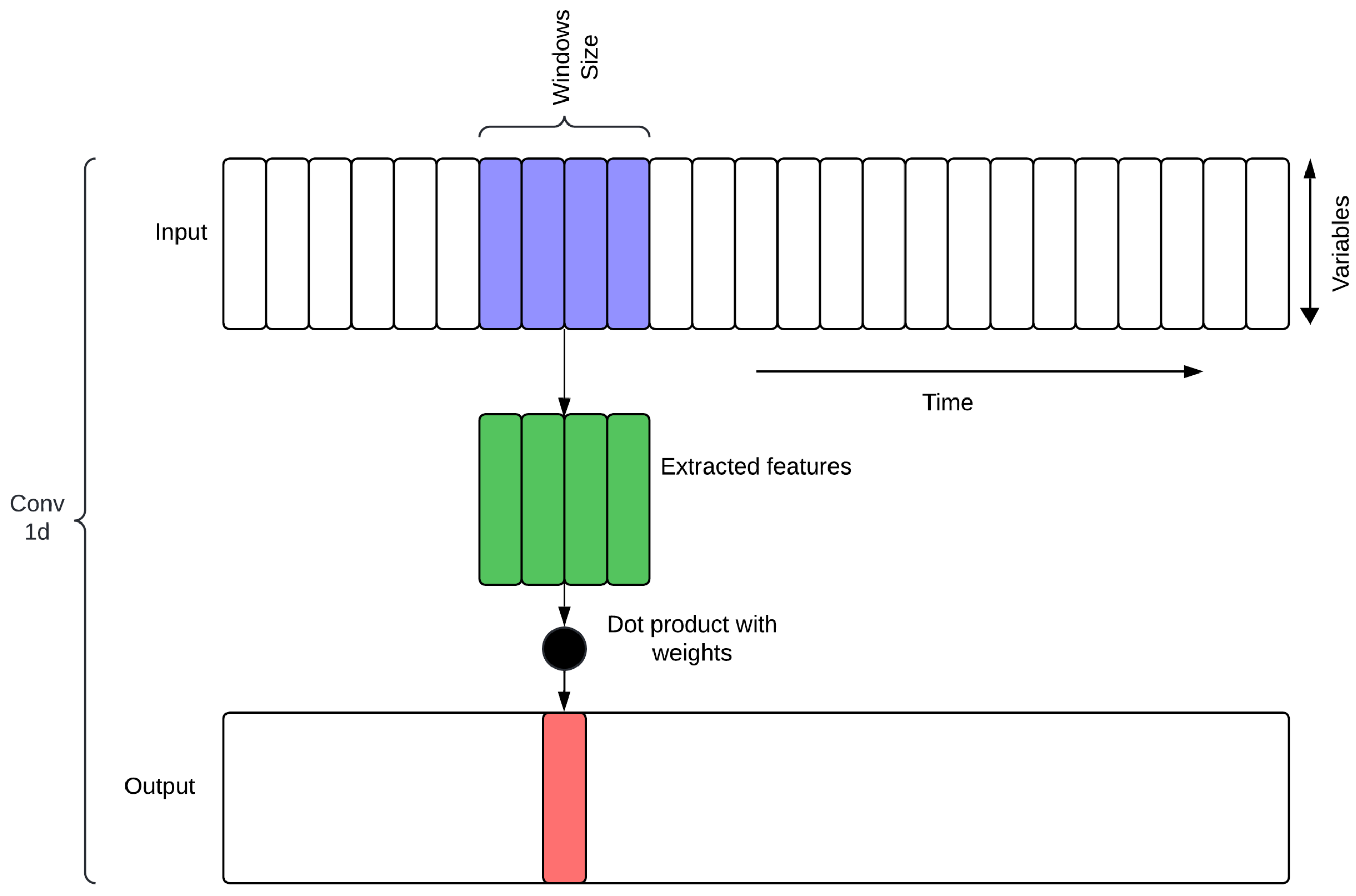
CNN models are versatile and capable of handling multiple input data formats, including 1D, 2D, and nD, where data typically consists of 1 to n channels [48]. This study employed a 1D input data format within the proposed hybrid model (see Figure 5). For this purpose, the time series data were treated as a one-dimensional grid, where each variable is represented as a distinct channel, allowing the CNN to learn the spatial relationships between variables while preserving the temporal sequence. The sliding window size should ensure that the model effectively captures the temporal features encountered. Therefore, our CNN has three convolutional layers, kernel sizes of 3, and stride of 1, which were optimized to balance computational efficiency and the ability to learn hierarchical patterns. This enables the CNN to extract meaningful features that are passed on to downstream components in the hybrid encoder-decoder model, improving the overall predictive accuracy of the model.

The application of CNNs in this research follows that in the cited literature, which the authors have used to extract and identify patterns in meteorological variables to improve solar irradiance forecasting. We intend to take advantage of the ability of CNNs to automatically learn hierarchical features from raw input data, such that the model could effectively capture complex temporal dependencies and spatial correlations within the data. The integration of CNNs into the hybrid model can complement other components by providing complex feature extraction, improving the overall predictive accuracy of solar irradiance forecasts.

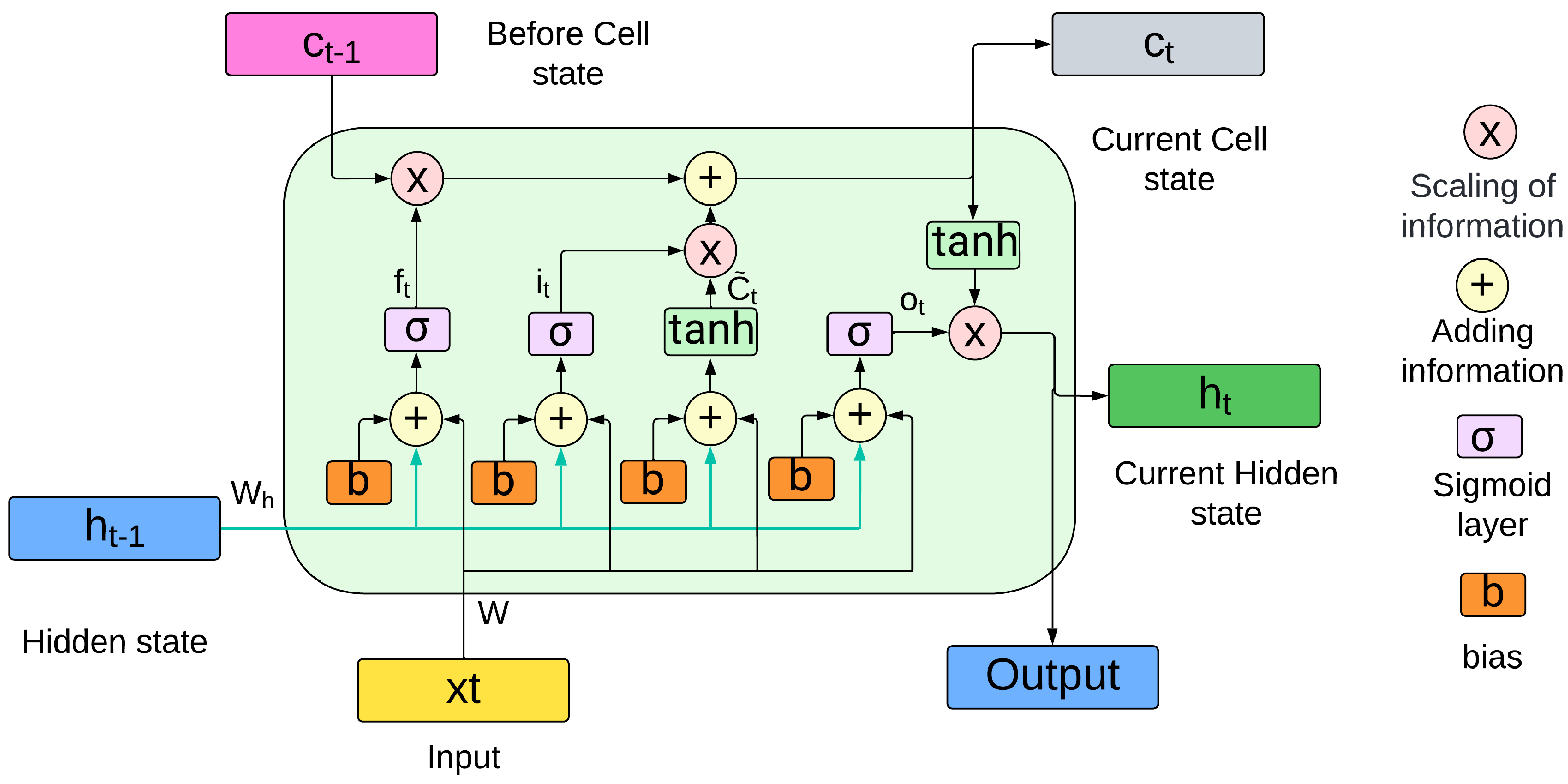
2.10. Long Short-Term Memory (LSTM)

The LSTMs depicted in Figure 6 are a variant of recurrent neural networks (RNNs). RNNs can process sequential data and maintain information over time, but basic RNNs need help with problems such as vanishing and gradient bursting, which complicate their ability to capture long-term dependencies [49,50]. Therefore, LSTMs were developed, which incorporate forget, input, and output gates, and an internal memory unit called the cell state. The forget gate is responsible for removing irrelevant information, the input gate updates the cell state with new information, and the output gate filters the current state to transmit the most important information. LSTMs has been shown in several papers to be highly effective for accurate forecasting in a variety of applications, including renewable energy.

The forget gate is calculated by the sigmoid function applied to the linear combination of the previous hidden state $h_{t-1}$ and the current input $x_t$, as shown in Equation (14).

$$\begin{array}{cc}\hfill f_t& =\sigma (W_f·[h_{t-1},x_t]+b_f)\hfill \end{array}$$

(14)

Next, the input gate is determined in a similar manner, as shown in Equation (15).

$$\begin{array}{cc}\hfill i_t& =\sigma (W_i·[h_{t-1},x_t]+b_i)\hfill \end{array}$$

(15)

The new candidate information for the memory cell is calculated using the hyperbolic tangent function (tanh), as shown in Equation (16).

$$\begin{array}{cc}\hfill {\tilde{C}}_t& =\tanh (W_C·[h_{t-1},x_t]+b_C)\hfill \end{array}$$

(16)

The state of cell $C_t$ is updated by combining the old information, modulated by the forgetting gate, with the new candidate information, weighted by the input gate, as described in Equation (17).

$$\begin{array}{cc}\hfill C_t& =f_t\ast C_{t-1}+i_t\ast {\tilde{C}}_t\hfill \end{array}$$

(17)

The output gate, which determines the part of the cell that should be passed to the next hidden state, is defined by Equation (18).

$$\begin{array}{cc}\hfill o_t& =\sigma (W_o·[h_{t-1},x_t]+b_o)\hfill \end{array}$$

(18)

Finally, the new hidden state $h_t$ is calculated by applying the function tanh to the cell state and multiplying by the gate output, as presented in Equation (19).

$$\begin{array}{cc}\hfill h_t& =o_t\ast \tanh \left(C_t\right)\hfill \end{array}$$

(19)

where, $W_f$, $W_i$, $W_C$, and $W_o$ are the weights associated with each gate, while $b_f$, $b_i$, $b_C$, and $b_o$ are the corresponding biases. The $\sigma$ function represents the sigmoid activation that regulates the flow of information in the gates, while tanh is used to generate the new memory units $C_t$ due to its ability to capture nonlinear relationships efficiently.

2.11. Multi-Head Attention Mechanism (ATT)

The ATT (see Figure 7) first presented by [51] was a new advance in DL architectures, especially in the transformer model. This mechanism has been used in several applications to improve learning capability [52]. This mechanism uses three main matrices: the query matrix Q, which represents the encoded temporal features to which attention is paid; the key matrix K, which represents the encoded features available for comparison; and the value matrix V, which contains the features used to compute the attention result. These matrices simultaneously focus on different parts of the input sequence, thus capturing a wide range of contextual information.

Mathematically, the ATT is defined as Equations (20) and (21).

$$\begin{array}{cc}\hfill \mathrm{MultiHead}(Q,K,V)& =\mathrm{Concat}({\mathrm{head}}_1,{\mathrm{head}}_2,\cdots ,{\mathrm{head}}_h)W^O\hfill \end{array}$$

(20)

$$\begin{array}{cc}\hfill {\mathrm{head}}_i& =\mathrm{Attention}(Q{W}_i^Q,K{W}_i^K,V{W}_i^V)\hfill \end{array}$$

(21)

where, Q, K, and V represent the query, key, and value matrices, respectively. The projection matrices $W_i^Q$, $W_i^K$, and $W_i^V$ correspond to each attention head i, and $W^O$ is the output projection matrix. The function Attention is defined as the scaled scalar product attention (see Equation (22)).

$$\begin{array}{cc}\hfill \mathrm{Attention}(Q,K,V)& =\mathrm{softmax}\left({\displaystyle \frac{Q{K}^T}{\sqrt{d_k}}}\right)V\hfill \end{array}$$

(22)

where $d_k$ denotes the dimensionality of the keys. The softmax function ensures that the attention weights are positive and their sum equals one, thus facilitating the effective weighting of values according to their relevance to queries.

We use this mechanism to improve the ability of our hybrid model to capture long-term dependencies and complex relationships in climate data. To this end, the ATT can identify hidden patterns and time-varying correlations. This results in more accurate and robust forecasts, especially for dynamic and seasonal features.

2.12. Positional Encoding and Embedding

Positional encoding is a technique that allows our hybrid model to incorporate temporal position information from the input sequences. This is useful to capture the sequentiality of time series data, which can be easily lost in ATT. On the other hand, the embedding layer maps the original input features, which represent variables such as irradiance, temperature and wind speed in a higher dimensional space, allowing the model to capture complex patterns and interactions between variables.

The embedding operation can be expressed as Equation (23).

$$\mathrm{Embedding}\_\mathrm{Out}=W_{embed}·Input+b_{embed}$$

(23)

where $Input$ represents the input feature vector, $W_{embed}$ is the embedding matrix, and $b_{embed}$ is the bias term.

Consequently, we add positional encoding so that we can add unique information about the time steps in the input sequence, with each position in the input sequence thus having a distinct time position. The positional encoding vector $PE$ of each time step is represented using sinusoidal functions (see Equations (24) and (25)).

$$P{E}_{(pos,2i)}=\sin \left({\displaystyle \frac{pos}{{10000}^{\frac{2i}{d_{model}}}}}\right)$$

(24)

$$P{E}_{(pos,2i+1)}=\cos \left({\displaystyle \frac{pos}{{10000}^{\frac{2i}{d_{model}}}}}\right)$$

(25)

where $pos$ is the position of the time step in the sequence, i represents the dimension, and $d_{model}$ is the dimensionality of the embedding space. Including of positional encoding allows the temporal structure of the data to be maintained, which is essential for the model to understand the temporal positions of the data in time-dependent problems, e.g., solar irradiance prediction.

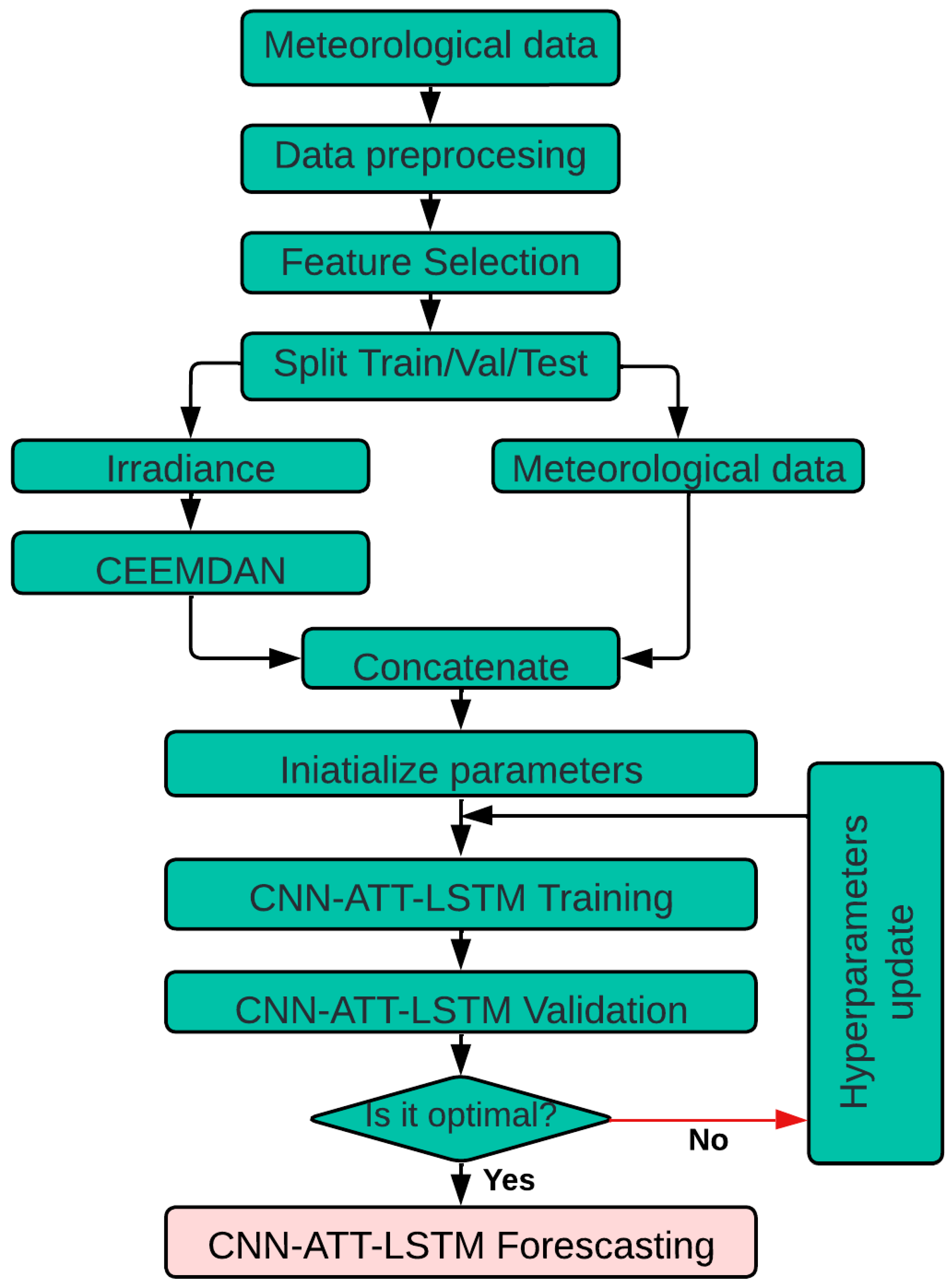
2.13. CEEMDAN-CNN-ATT-LSTM Model

Figure 8 presents a hybrid achitecture for solar radiance forecasting that combines CNNs, LSTM networks, and an ATT for solar irradiance forecasting. This combination leverages the strengths of each component: CNNs for spatial feature extraction, LSTMs to capture short-term temporal dependencies, and an ATT to extract long-term patterns from the input sequence.

Our proposed CEEMDAN-CNN-ATT-LSTM model employs a carefully designed architecture with specific hyperparameters to optimize its performance. The CNN encoder consists of three sequential 1D convolutional layers. The first convolutional layer has 256 filters, the second 128 filters, and the third 256 filters, each with a kernel size of 3 and a padding of 1 to preserve the input size. Batch normalization is introduced after each convolutional layer to stabilize and speed up training. In addition, dropout regularization with a specific probability is applied after each layer to avoid overfitting. After the last convolutional layer, a ReLU activation function is applied to introduce nonlinearity. The goal of this setup is to extract spatial features from the input data while maintaining local temporal dependencies.

The LSTM component includes two stacked LSTM layers with 256 hidden units each. A dropout regularization with a rate of 0.2 is applied between the layers to mitigate overfitting and improve generalization. The outputs of the LSTM layers are normalized using layer normalization to stabilize the training.

For ATT, eight attention heads were employed, each with a projection dimension of 64. This design allows the model to focus on different parts of the input sequence simultaneously, effectively capturing both short- and long-term dependencies. Positional coding is added to maintain temporal order within the input sequence, ensuring that the model correctly interprets the sequential nature of the data.

The final dense layer consists of 128 units, followed by a single output unit with a sigmoid trigger function to produce normalized forecasting. This ensures that the output is limited to a range suitable for forecasting solar irradiance.

The model input is the sequence of irradiance data preprocessed using the CEEMDAN decomposition. In addition to irradiance, variables such as temperature and air humidity are included. Mathematically, the input x is a tensor $x\in {\mathbb{R}}^{q\times n}$, where q is the sequence length (number of time points) and n is the number of features (in this case, 19 features). The input shape is $(batch\_size,q,n)$.

Three cascaded 1D convolutional layers are applied in the encoder, each using filters to extract local features from the input sequence. Each convolutional layer’s input x consists of the irradiance and other meteorological variables for each time step. The convolution operation is expressed in Equation (26).

$${\mathrm{Conv}\_\mathrm{Out}}_l=ReLU(W_{con{v}_l}\ast x+b_{con{v}_l})$$

(26)

where ${\mathrm{Conv}\_\mathrm{Out}}_l$ is the output of the l-th convolutional layer, $W_{con{v}_l}\in {\mathbb{R}}^{k\times n\times m}$ are the weights (with k being the kernel size, n the input feature dimension, and m the output feature dimension), $b_{con{v}_l}\in {\mathbb{R}}^m$ are the biases, and ∗ denotes the convolution operation. The ReLU activation function introduces non-linearity to the output, allowing the model to learn complex patterns in the data.

Following each convolutional layer, average pooling is applied to reduce the dimensionality of the feature maps and prevent overfitting. This operation is defined in Equation (27).

$${\mathrm{Pooled}\_\mathrm{Out}}_l={\displaystyle \frac{1}{n_{pool}}}\sum _{i=1}^{n_{pool}}{\mathrm{Conv}\_\mathrm{Out}}_{l,i}$$

(27)

where ${\mathrm{Pooled}\_\mathrm{Out}}_l$ is the pooled output from the l-th layer, and $n_{pool}$ is the pooling window size. After pooling, batch normalization is applied to standardize the outputs, as shown in Equation (28).

$${\mathrm{Normalized}\_\mathrm{Out}}_l={\displaystyle \frac{{\mathrm{Pooled}\_\mathrm{Out}}_l-{\mu }_l}{\sqrt{{\tau }_l^2+\psi }}}$$

(28)

where ${\mu }_l$ and ${\tau }_l^2$ are the mean and variance of the output from the l-th layer, and $\psi$ is a small constant for numerical stability.

The features extracted by the CNN are then passed through two LSTM layers. The input to each LSTM layer consists of the normalized outputs from the previous stage, which are data sequences representing features over time. The LSTM operation is given in Equation (29).

$$h_t=\mathrm{LayerNorm}\left(\mathrm{Dropout}\left(\mathrm{LSTM}\left({\mathrm{Normalized}\_\mathrm{Out}}_l\right)\right)\right)$$

(29)

where LayerNorm represents layer normalization, and Dropout is used to prevent overfitting. The hidden units in this LSTM layer are set to 256. The LSTM layer captures the temporal dependencies in the data, with $h_t$ being the output at time step t.

ATT is then applied to the outputs of the two LSTM layers and the positional encoding (see Equation (30)). The attention layer calculates the importance of each time step in the sequence, helping the model focus on the most relevant features for predicting solar irradiance. This is expressed in Equation (31).

$$h_{tpos}=\mathrm{Positional}\_\mathrm{Encoding}\left(h_t\right)$$

(30)

$${\mathrm{Attention}\_\mathrm{Out}\_\mathrm{enc}}_t=\mathrm{MultiHead}(h_{tpos},h_{tpos},h_{tpos})$$

(31)

Residual connections are then employed (see Equation (32)) to add the original input back to the output of the attention mechanism:

$$h{t}_{enc}={\mathrm{Attention}\_\mathrm{Out}\_\mathrm{enc}}_t+h_{tpos}$$

(32)

This technique helps to maintain the original input information, enhancing the stability and performance of the model.

Before applying the ATT in the decoder, the target history (i.e., historical irradiance data) is embedded to map the input features into a higher-dimensional space that can capture more complex patterns. The embedding operation is described in Equation (33).

$$\mathrm{Embedding}\_\mathrm{Out}=\mathrm{Embedding}\left(\mathrm{Target}\_\mathrm{History}\right)$$

(33)

where $\mathrm{Target}\_\mathrm{History}\in {\mathbb{R}}^q$ represents the sequence of past irradiance values, and Embedding is the operation that transforms these values into a higher-dimensional space $\mathrm{Embedding}\_\mathrm{Out}\in {\mathbb{R}}^{q\times d}$, where d is the embedding dimension.

To incorporate temporal information into the sequence, positional encoding is added to the embedded target history. This process is shown in Equation (34).

$$hi{s}_{pos}=\mathrm{Positional}\_\mathrm{Encoding}\left(\mathrm{Embedding}\_\mathrm{Out}\right)$$

(34)

The positional encoding allows the model to differentiate between the positions of time steps in the sequence, which is crucial for tasks involving sequential data.

A multi-head attention mechanism is then applied to the outputs of the encoder and the positional encoded target history. This is expressed in Equation (35).

$${\mathrm{Attention}\_\mathrm{Out}}_t=\mathrm{MultiHead}(hi{s}_{pos},h{t}_{enc},h{t}_{enc})$$

(35)

Then, residual connections are employed to add the original input back to the output of the ATT (See Equation (36)).

$$\mathrm{Residual}\_\mathrm{Out}=\mathrm{Positional}\_\mathrm{Encoded}\_\mathrm{Out}\left({\mathrm{Attention}\_\mathrm{Out}}_t\right)$$

(36)

The features extracted are then passed through two LSTM layers. The LSTM operation is given in Equation (37).

$$\mathrm{LSTM}\_\mathrm{Out}=\mathrm{LayerNorm}\left(\mathrm{Dropout}\left(\mathrm{LSTM}\left({\mathrm{Residual}\_\mathrm{Out}}_l\right)\right)\right)$$

(37)

The output from the LSTM is flattened into a one-dimensional vector, as shown in Equation (38).

$$\mathrm{Flatten}\_\mathrm{Out}=\mathrm{reshape}\left(\mathrm{LSTM}\_\mathrm{Out}\right)$$

(38)

This vector is then passed through a fully connected layer to produce the final prediction (See Equation (39)).

$$y_{pred}=W_{fc}·\mathrm{Flatten}\_\mathrm{Out}+b_{fc}$$

(39)

where $W_{fc}$ and $b_{fc}$ are the weights and biases of the fully connected layer, and $y_{pred}$ is the predicted solar irradiance value. The output is then passed through a sigmoid function to constrain the predictions (See Equation (40))

$$y_{final}=\sigma \left(y_{pred}\right)={\displaystyle \frac{1}{1+e^{-y_{pred}}}}$$

(40)

where $\sigma \left(y_{pred}\right)$ represents the sigmoid activation applied to the predicted value to ensure non-negative output.

Algorithms 1 and 2 describe the training and forecasting process of the hybrid model developed for this task. In the first phase, the model is iteratively trained on a dataset, adjusting its parameters to minimize a loss function represented as $\mathcal{L}$. During each epoch, the model is evaluated on a validation set to ensure that it learns from the training data and generalizes well to new data. The prediction phase, which follows training, uses the optimized model to generate predictions on test data.

Algorithm 1: Training and Prediction with CNN-LSTM-MultiHeadAttention Model

1: Input: Time series data $\mathbf{X}=[{\mathbf{x}}_1,{\mathbf{x}}_2,\dots ,{\mathbf{x}}_T]\in {\mathbb{R}}^{T\times v}$, where T is the time series length, v is the number of variables, and $\mathbf{h}$ is the history of irradiance. 2: Step 1: CEEMDAN Decomposition of Irradiance 3:    Initialize CEEMDAN parameters: trials, noise level, siftings 4:    Apply CEEMDAN to decompose the irradiance data $\mathbf{h}$ into Intrinsic Mode Functions (IMFs) and a residue 5:    Append IMFs and residue to the feature set $\mathbf{X}$ 6: Initialize: 7:     Load configuration parameters: hidden layers $hl$, batch size $bs$, epochs e, patience p 8:     Initialize model $M=model\left(hyperparameters\right)$ 9:     Apply weight initialization $M.apply(initialize\_weights)$ and move model to device 10:    Define loss criterion $\mathcal{L}=\mathrm{L}1\mathrm{Loss}\left(\right)$ 11:    Define optimizer $O=\mathrm{Adam}(M.parameters(),lr=Lr)$ and scheduler 12:    Initialize variables: best_val_loss = ∞, patience_counter = 0 13:    Load $X_{training}$, $X_{test}$, $X_{val}$ and irradiance history h 14: Create DataLoader iterators for training, validation, and test data with batch size $bs$ 15: for each epoch e do 16:    Training Phase: 17:       Set model to training mode 18:       Initialize training loss to zero 19:    for each batch in $X_{training}$ do 20:         Zero the parameter gradients 21:         $output=M(inputs,h)$ 22:         Compute loss $\mathcal{L}=criterion(output,targets)$ 23:         Add L1 regularization ${\mathcal{L}}_{reg}=\mathcal{L}+\lambda ·L{1}_{norm}\left(params\right)$ 24:         Perform backpropagation ${\mathcal{L}}_{reg}.backward\left(\right)$ 25:         Clip gradients and update model parameters 26:         Accumulate training loss ${\mathcal{L}}_{train}+={\mathcal{L}}_{reg}$ 27:    end for 28:       Compute average training loss ${\mathcal{L}}_{train\_avg}={\mathcal{L}}_{train}/\mathrm{number}\mathrm{of}\mathrm{batches}$ 29:    Validation Phase: 30:       Set model to evaluation mode 31:       Initialize validation loss to zero 32:    for each batch in $X_{val}$ do 33:         Disable gradient computation 34:         $outpu{t}_{val}=M(val\_inputs,val\_history)$ 35:         Compute loss ${\mathcal{L}}_{val}=criterion(outpu{t}_{val},val\_targets)$ 36:         Accumulate validation loss ${\mathcal{L}}_{val}+={\mathcal{L}}_{val}$ 37:    end for 38:       Compute average validation loss ${\mathcal{L}}_{val\_avg}={\mathcal{L}}_{val}/\mathrm{number}\mathrm{of}\mathrm{batches}$ 39:    Early Stopping: 40:    if ${\mathcal{L}}_{val\_avg}<$ best_val_loss then 41:         Update best_val_loss $={\mathcal{L}}_{val\_avg}$ 42:         Save model parameters and reset patience_counter $=0$ 43:    else 44:         Increment patience_counter $+=1$ 45:    end if 46:    if patience_counter $>p$ then 47:         Break training loop early 48:    end if 49: end for

Algorithm 2: Prediction with CNN-LSTM-MultiHeadAttention Model

1: Test the model using $X_{test}$ 2:    Set model to evaluation mode 3:    Initialize test loss to zero 4:    Initialize lists for predictions, actual values, and dates 5: for each batch in $X_{test}$ do 6:       Disable gradient computation 7:       $outpu{t}_{test}=M(test\_inputs,test\_history)$ 8:       Compute test loss ${\mathcal{L}}_{test}=criterion(outpu{t}_{test},test\_targets)$ 9:       Accumulate test loss ${\mathcal{L}}_{test}+={\mathcal{L}}_{test}$ 10:      Store predictions and actual values for future analysis 11: end for 12:    Compute average test loss ${\mathcal{L}}_{test\_avg}={\mathcal{L}}_{test}/\mathrm{number}\mathrm{of}\mathrm{batches}$ 13:    Post-processing: 14:    Apply EWMA smoothing to the test loss 15:    Apply sliding window anomaly detection to identify possible faults 16:    Compute evaluation metrics: RMSE, MAE, R2, MAPE 17:    Save predictions, actual values, and metrics for reporting 18: Output: 19:    Final model performance metrics and saved model for deployment or further analysis

2.14. Data Splitting

The dataset was divided into two parts for the forecasting model’s input, taking into account the area’s specific climatic conditions, which have two distinct seasons: summer and winter. Since we have data for an entire year, different periods are used for the model’s training, validation, and testing.

For the winter season, data from December to May 2023 are used for training, January 2024 for validation, and February 2024 for testing the model with unseen data. As for the summer season, data from December to May 2023 are used for training, July 2024 for validation, and August 2024 for testing. This strategy considers seasonal variations, which can significantly affect the model’s accuracy.

2.15. Model Hyperparameters

Table 5. Hyperparameters used in CNN-ATT-LSTM.

Hyperparameter	Value
Sequence length	144
Length of prediction	4 (2 h), 24 (12 h)
Batch size	128
Hidden dimension (CNN LSTM & ATT)	256
Kernel Size (CNN)	3
Stride (CNN)	2
Padding (CNN)	1
Output dimension	1
Number of LSTM layers	3
Number of encoder/decoder layers	1
Attention mechanisms	8
Dropout probability	0.1
Learning rate	0.00001
Learning rate factor	0.25
Epochs with max learning rate	3
Total epochs	100
Patience for early stopping	10
Time resampling interval	10 min, 30 min and 1 h
Target variable	Solar irradiance (W/m2)

shows the hyperparameters used in the hybrid model. The hyperparameters shown in the table were selected because they obtained the best model performance. The sequence length and model prediction were set to 144, allowing the model to process data sequences of 144 units. A batch size 128 was used to balance computational efficiency and training stability. The model includes 2 LSTM layers, allowing temporal dependencies in the data to be more effectively captured. In addition, 8 attention mechanisms were implemented to improve the model’s ability to focus on relevant parts of the sequence. Finally, 3 convolutional layers were added to extract additional spatial features from the data.

2.16. Model Evaluation Metrics

We use different common error metrics in forecasting models to evaluate the proposed model. These metrics include the root mean square error (RMSE), the mean absolute error (MAE), the mean absolute percentage error (MAPE), and the coefficient of determination ($R^2$). In Equations (41)–(44) we define these metrics.

• Root mean square error (RMSE): RMSE calculates the square root of the mean of the squared differences between the predicted values (${\widehat{y}}_i$) and the actual values ($y_i$). It is highly sensitive to large errors, as these are squared before averaging. A lower RMSE indicates higher predictive accuracy, and a value of zero would represent a perfect model. RMSE is calculated as in Equation (41).

  $$\mathrm{RMSE}=\sqrt{{\displaystyle \frac{1}{n}}\sum _{i=1}^n{(y_i-{\widehat{y}}_i)}^2}$$

  (41)
• Mean absolute error (MAE): MAE is defined as in Equation (42). This metric calculates the mean of the absolute differences between predicted and actual values. In contrast to RMSE, MAE does not penalize large errors so heavily and so it is a good option when a metric that treats all errors equally is required. A lower MAE indicates better model performance.

  $$\mathrm{MAE}={\displaystyle \frac{1}{n}}\sum _{i=1}^n|y_i-{\widehat{y}}_i|$$

  (42)
• Mean absolute percentage error (MAPE): MAPE is the mean of the absolute percentage errors between the forecast and actual values. A lower MAPE indicates that the forecast is closer to the observed values. However, one disadvantage of MAPE is that when actual values tend toward zero, they typically become extremely large, leading to disproportionately large values. Its calculation is based on Equation (43).

  $$\mathrm{MAPE}={\displaystyle \frac{1}{n}}\sum _{i=1}^n\left|{\displaystyle \frac{y_i-{\widehat{y}}_i}{y_i}}\right|\times 100$$

  (43)
• Coefficient of determination ($R^2$): $R^2$, defined in Equation (44), measures the proportion of the variance in the dependent variable that is predictable from the independent variables. A value $R^2$ close to 1 indicates that the model accurately predicts the target variable. In contrast, a value $R^2$ close to 0 indicates that the model does no better than the mean of the target values.

  $$R^2=1-{\displaystyle \frac{{\sum }_{i=1}^n{(y_i-{\widehat{y}}_i)}^2}{{\sum }_{i=1}^n{(y_i-\overline{y})}^2}}$$

  (44)

In Equations (41)–(44), $y_i$ represents the actual values, ${\widehat{y}}_i$ represents the predicted values, n is the number of samples, and $\overline{y}$ is the mean value of $y_i$.

To conclude this section, the experiments were conducted using the Python programming language (version 3.11.11) in the PyTorch library (version 2.5.1+cu121) within a Google Colab environment. The environment comprised an Intel(R) Xeon(R) CPU @ 2.20 GHz (Intel, Santa Clara, CA, USA), 51.00 GB of RAM, a Tesla K80 accelerator (Tesla, Austin, TX, USA), and 12 GB of GDDR5 VRAM.

3. Results

This section presents the results for the winter and summer seasons, considering different forecasting time horizons at 1 h, 6 h, and 12 h. In addition, the analyses performed for different temporal resamples are included. The results are compared to the base models, providing an evaluation of the proposed model’s performance compared to traditional approaches.

Table 6. Losses and training time by epoch for each architecture component with 1 h resampling for 12 h forecast in summer.

Model	MAE	RMSE	${\mathit{R}}^2$	Train/Epoch (s)
Our model + CEEMDAN	110.43	141.27	0.63	2.71
Model + Wavelet	120.03	147.50	0.61	2.60
Model without attention mechanisms	126.36	145.32	0.60	2.42
Model without encoder-decoder and history	132.61	150.46	0.58	2.30
Baseline LSTM model	135.75	133.69	0.55	1.95

summarizes the losses obtained using various configurations of our solar radiation forecasting model, evaluated from 12 h forecasts. Our model shows an MAE of 110.43 and a $R^2$ of 0.63, indicating solid performance compared to the models without the proposed configurations. The “Model + Wavelet” configuration achieves an MAE of 120.03 and an $R^2$ of 0.61, demonstrating reasonable performance but falling short of the CEEMDAN-enhanced model, particularly in capturing intricate variability in solar irradiance data. The “Model without attention mechanisms” yields an MAE of 126.36 and an $R^2$ of 0.60, suggesting a slight reduction in accuracy when attention mechanisms are removed. The “Model without encoder-decoder and history” shows an MAE of 132.61 and an $R^2$ of 0.58, reflecting a further loss of accuracy when both historical data and the encoder-decoder structure are excluded. Finally, the “Baseline LSTM model” yields an MAE of 135.75 and an $R^2$ of 0.55, indicating a lower explanatory power than the other models.

The execution time of our proposed model was evaluated for 12 h forecasts using the hyperparameters outlined in Table 5 with a 1 h resampling interval. Figure 9 shows that the average iteration time was measured across different batch sizes. A batch size of 256 significantly increased iteration time due to processing more data, while a batch size of 64 reduced iteration time by handling fewer data points. However, it is worth noting that in this case, the larger the batch size, the less training time we obtain by sacrificing model accuracy. We selected a batch size of 128, as it balances computational efficiency and performance, particularly with eight attention heads. Analysis of dropout rates revealed that values of 0.01 and 0.3 exhibited similar iteration times (0.55 and 0.57 s, respectively). Regarding attention heads, configurations with four heads were slightly faster than those with eight heads. Larger hidden sizes increased iteration time compared to a hidden size of 128, reflecting the higher computational demands of more extensive representations. Similarly, increasing the number of layers led to longer training times due to more computations per iteration. The learning rate had minimal impact on run time, although it significantly affected model accuracy, as will be discussed later. In addition, longer sequence lengths resulted in more complex architectures and exponentially increased training time.ased training time.

Figure 10 presents the loss rates during training and validation across different hyperparameters, including the number of layers, sequence length, and learning rate. From these plots, it can be observed that, in some cases, the loss during training is slightly higher than during validation. This indicates that the model is effectively learning the underlying patterns in the data without overfitting, showcasing its robustness. Specifically, the model was tested with one, two, and three LSTM layers (see Figure 10a), with the best performance being achieved with three layers during both training and validation phases, establishing this configuration in our model. Subsequently, varying the sequence length between 10, 40, 72, and 144 time steps (see Figure 10b), we observed optimal performance with sequence lengths of 40 and 72, corresponding to 40 h (2 days) and 72 h (3 days), respectively. We selected a sequence length of 72 time steps, as it effectively represents a 3-day period. The learning rate (see Figure 10c) was also tuned, with values set at $1\times {10}^{-4}$, $1\times {10}^{-5}$, and $1\times {10}^{-6}$. It was observed that a learning rate of $1\times {10}^{-4}$ yielded better performance with appreciable improvements. Figure 10d, shows that increasing the number of attention heads improves the performance of the model; therefore, we selected a configuration with eight attention heads, achieving superior performance in both the training and validation phases. Figure 10e illustrates the evaluation of different dropout rates. Dropout values of 0.1 and 0.001 perform well during the training process, stabilizing to deliver optimal performance. On the other hand, a dropout rate of 0.3 results in highly erratic behavior, leading to suboptimal results. Consequently, we selected a dropout rate of 0.1 as the most suitable value for our model. In Figure 10f, we observe that batch sizes of 128 and 64 provide stable training performance, with the distinction that the training process is slower for a batch size of 64. Conversely, a batch size of 256, while faster, does not yield satisfactory results in terms of accuracy. Therefore, we selected a balanced approach with a batch size of 128. Additionally, Figure 10g highlights that hidden sizes of 128 and 256 provide stability for our model. While a hidden size of 512 shows potential for better performance, it requires significantly more time to train over 50 epochs. To achieve a balance between training efficiency and performance, we chose a hidden size of 256 for our final model configuration.

3.1. Forecasting at 1 h Ahead with Different Resampling for Winter and Summer

Figure 11 depicts the 1 h ahead predictions achieved for different resampling configurations in winter (left column) and summer (right column). In general, in comparison with winter, the model makes more accurate summer predictions, as inferred from the error metrics. For the 10 min resampling in winter (Figure 11a), the MAE equates to 111.31, the RMSE equals 148.62, and the $R^2$ is 0.50, while for the same configuration in summer (Figure 11b), it has increases. For the 30 min resampling, the model achieves an MAE of 109.64, an RMSE of 147.07, and an $R^2$ of 0.44 under winter conditions (Figure 11c). On the other hand, under summer conditions (Figure 11d), the model results are an MAE 114.45, an RMSE of 146.83, and an $R^2$ is 0.63. In winter (Figure 11e), the MAE is 116.47, the RMSE is 148.78, and the $R^2$ is 0.59, whereas in summer (Figure 11f), the MAE decreases to 100.22, the RMSE to 135.15, and the $R^2$ to 0.46. This suggests that the model is more accurate during summer in estimating solar irradiance, especially for larger resampling intervals, and remains reasonably accurate in winter.

3.2. Forecasting at 6 h Ahead with Different Resampling for Winter and Summer

Figure 12 represents the 6 h ahead predictions with different resampling configurations. The figures on the right represent the summer, and those on the left represent the winter. The results show how the model performs under these resampling configurations, considering the effect of seasonal variations. For the 10 min resampling in winter (Figure 12a), the MAE is 117.39, the RMSE is 169.62, and the $R^2$ is 0.35, indicating moderate performance for a 6 h prediction. The resampling in summer (Figure 12b) yields an MAE of 222.91, an RMSE of 275.98, and a negative $R^2$ of −0.17, reflecting lower prediction accuracy due to increased seasonal variability. During winter (Figure 12c), the RMSE is 151.30, the MAE is 107.95, and the $R^2$ improves to 0.42, showing enhanced accuracy with a larger resampling interval. During summer (Figure 12d), the RMSE is 161.69, the MAE is 119.14, and the $R^2$ improves to 0.55, indicating better prediction accuracy. In winter (Figure 12e), the MAE is 100.12, the RMSE is 134.13, and the $R^2$ is 0.48, reflecting better accuracy in long-term forecasts compared to smaller resampling intervals. In summer, the RMSE decreases to 141.15, the MAE to 110.43, and the $R^2$ reaches 0.64, reflecting the model’s ability to capture seasonal patterns in long-term predictions with larger resampling intervals.

3.3. Forecasting at 12 h Ahead with Different Resampling for Winter and Summer

Figure 13 presents the results of 12 h ahead forecasts with varying resampling intervals, comparing winter (left column) and summer (right column). For the 10 min resampled forecasts in winter (Figure 13a), the model achieves an MAE of 116.46, an RMSE of 173.08, and an $R^2$ of 0.33, indicating moderate accuracy. However, in summer (Figure 13b), the error increases significantly with an MAE of 218.22, an RMSE of 266.95, and a negative $R^2$ of −0.09, reflecting higher seasonal variability. The 30 min resampled results in winter (Figure 13c) improve slightly, with an MAE of 112.63, an RMSE of 154.51, and an $R^2$ of 0.39, showing better accuracy over longer intervals. For summer (Figure 13d), the model achieves an MAE of 128.85, an RMSE of 160.40, and an $R^2$ of 0.56, indicating an improvement in forecast precision compared to shorter resampling intervals. Finally, for the 1 h resampling, the winter predictions (Figure 13e) demonstrate a significant increase in accuracy, with an MAE of 99.89, an RMSE of 130.42, and an $R^2$ of 0.51, while the summer predictions (Figure 13f) also show improved results, with an MAE of 110.43, an RMSE of 141.15, and an $R^2$ of 0.64. These results show that larger resampling intervals improve forecast accuracy, especially over longer prediction horizons such as 12 h ahead.

Table 7. Comparison of metrics for irradiance prediction with different resampling and forecast horizons.

Resampled	Metric	Time Interval
		1 h	6 h	12 h
10 min (Winter)	MAE	111.31	117.39	116.46
	RMSE	148.62	169.62	173.08
	$R^2$	0.50	0.35	0.33
	MAPE	1,737,572.90	1,438,205.13	892,101.04
10 min (Summer)	MAE	116.10	222.91	218.22
	RMSE	147.68	275.98	266.95
	$R^2$	0.66	−0.17	−0.09
	MAPE	1,865,474.68	4,790,196.73	4,305,417.09
30 min (Winter)	MAE	109.64	107.95	112.63
	RMSE	147.07	151.30	154.51
	$R^2$	0.44	0.42	0.39
	MAPE	650.25	546.71	645.45
30 min (Summer)	MAE	114.45	119.14	128.85
	RMSE	146.83	161.69	160.40
	$R^2$	0.63	0.55	0.56
	MAPE	251.63	227.55	281.15
1 h (Winter)	MAE	116.47	100.12	99.89
	RMSE	148.78	134.13	130.42
	$R^2$	0.59	0.48	0.51
	MAPE	127.96	173.36	172.79
1 h (Summer)	MAE	100.22	110.30	110.43
	RMSE	135.16	146.13	141.15
	$R^2$	0.46	0.61	0.64
	MAPE	157.99	126.76	144.51

summarizes the performance metrics for irradiance prediction at different resampling intervals (10 min, 30 min, and 1 h) and forecast horizons (1 h, 6 h, and 12 h) for both winter and summer seasons. The metrics presented include the MAE, RMSE, $R^2$, and MAPE. The table shows that the model’s accuracy generally decreases with longer forecast horizons, especially in summer, where the higher seasonal variability leads to larger MAE and RMSE values. The best results are typically observed in the 1 h resampling, particularly for winter, where the MAE and RMSE values are the lowest for the 12 h ahead forecast. These results highlight the impact of both resampling intervals and forecast horizons on the overall prediction accuracy of the model, with winter predictions demonstrating higher accuracy than summer predictions across all time intervals.

Table 8. Comparison of metrics for 12 h ahead irradiance prediction in winter and summer with 1 h resampling.

Model	Metric	Season
		Winter	Summer
Our Model	MAE	116.47	110.43
	RMSE	148.78	135.16
	$R^2$	0.59	0.64
	MAPE	127.96	157.99
Baseline LSTM	MAE	120.52	115.32
	RMSE	151.89	140.21
	$R^2$	0.55	0.60
	MAPE	130.25	162.35
Autoencoder	MAE	118.73	112.57
	RMSE	150.03	137.98
	$R^2$	0.57	0.62
	MAPE	129.45	160.84
Transformer	MAE	118.00	113.50
	RMSE	148.50	140.75
	$R^2$	0.56	0.61
	MAPE	132.50	158.25

Note: In bold are the best results.

presents the performance metrics for forecasting irradiance 12 h in advance in winter and summer, with 1 h resampling intervals. The results compare the proposed model with a reference LSTM, an autoencoder, and a transformer-based model. The transformer model is configured with three encoder layers, three decoder layers, and eight attention heads. The proposed model outperforms the other approaches on MAE and $R^2$, showing higher accuracy, especially in summer, where it achieves an MAE of 110.43 and an $R^2$ of 0.64. The transformer model, while competitive, exhibits slightly higher MAE and RMSE values (118.00 and 148.50 in winter; 113.50 and 140.75 in summer) and a slightly lower $R^2$ (0.56 in winter and 0.61 in summer) compared to the proposed model. Both the reference LSTM and the autoencoder show slightly higher errors in both seasons, highlighting the proposed model’s greater efficiency for accurate irradiance forecasting under varying seasonal conditions. The RMSE and MAPE values confirm the proposed model’s robustness and performance compared to the alternatives, with the transformer model demonstrating robust performance, albeit with marginally higher error metrics.

Figure 14 shows two box plots illustrating the MAE distribution for solar irradiance forecasting at different horizons: 1 h, 6 h and 12 h. Figure 14a shows the summer forecast errors and Figure 14b the winter ones. Each box illustrates the MAE interquartile limits, and the red line within each box the MAE mean. The overall dispersion of the MAE is greater as the forecast horizon increases, as illustrated by the boxes for the 6 h and 12 h horizons. This, in turn, is consistent with expectations: longer forecast windows imply more significant uncertainty. However, despite this variability, the median MAE is reasonably stable over all horizons, including winter, which is reflective of the robustness of the model also for long-term forecasts. The difference in errors for the summer and winter seasons can be attributed to the seasonal effect, as summer tends to have a more compact error distribution than winter.

4. Conclusions

This research presents a novel methodology for forecasting solar irradiance in complex areas, combining advanced techniques such as a CEEMDAN, CNNs, attention mechanisms, and LSTM networks in a hybrid architecture. We integrated a CEEMDAN to decompose the solar irradiance variable into more interpretable components, which facilitated the identification of specific patterns in different time zones. The CEEMDAN proved effective in improving the accuracy of the forecasts in our model, providing a robust solution for integrating solar energy into the power grid and outperforming traditional approaches in terms of accuracy and generalization.

Our CEEMDAN-CNN-ATT-LSTM model demonstrated its ability to handle the variability and uncertain behavior of solar irradiance by combining the strengths of CNNs to capture spatial relationships between variables, the ability of LSTM networks to extract short-term temporal information, and the integrated attention mechanism to improve the ability to capture long-term spatial and temporal relationships by focusing on the most critical long-term features. This combination makes the model robust and allows it to generalize the time series to data with high variability, such as the high-altitude regions of southern Ecuador. In addition, the model is adaptable and can be applied to regions with more stable conditions.

Our model obtained an encouraging performance, with an MAE of 99.89 W/m² in winter and 110 W/m² in summer for a 12 h forecast, covering the entire diurnal solar cycle. The model was found to perform better when the time series was less variable, highlighting the importance of the resampling approach used in this study. Although our study obtained promising results, we found some limitations that we will address in the future, such as the dependence on the quality and quantity of the data used. In addition, the computational complexity of our hybrid model requires advanced hardware, such as GPU and sufficient RAM, which may cause problems in resource-constrained environments. Moreover, variations in the availability and quality of data from different regions or time periods can also affect the generalizability and performance of the model.

In the future, more advanced techniques will be adopted to optimize the speed and generalizability of the model, such as the use of transformer-like techniques. To this end, we will test its robustness in the case of stable and highly variable geographical regions and climatic conditions. In addition, we will include other related variables to increase the accuracy and reliability of the forecasting by adding weather forecasts and atmospheric parameters. Finally, such a model can be implemented within the operational structure, interfacing with real-time solar power generation systems, and be part of a grid connection with various performance optimization and adaptability options. Thus, the proposed approach will help the scientific community in the solar energy field to improve the methodological improvement of forecasting model building, with applicability in various scenarios to develop more accurate and efficient models in unpredictable and variable weather conditions.