Abstract
Branched horizontal wells are widely applied in oil and gas development. However, their complex structures make cuttings transport and deposition problems more pronounced. In this study, a three-dimensional branched wellbore model was established based on an intelligent drilling and completion simulation system. A computational fluid dynamics (CFD) approach, incorporating the Eulerian–Eulerian two-fluid model and the kinetic theory of granular flow, was employed to investigate the effects of wellbore diameter, eccentricity, curvature, flow rate, and rheological parameters on cuttings transport behavior. Results from the steady-state simulations indicate that increasing the wellbore diameter and eccentricity intensifies cuttings deposition at the connection section, with the lower-region concentration rising significantly as the eccentricity increases from 0% to 60%. A larger curvature enhances local flow disturbance but reduces the overall cuttings transport efficiency. Increasing the flow rate improves hole cleaning but may promote cuttings accumulation near the bottom of the main wellbore. As the flow behavior index increases from 0.4 to 0.8, the average cuttings concentration rises from 0.0996 to 0.1008, and the pressure drop increases from 1,010,894 Pa to 1,042,880 Pa, indicating improved transport capacity but higher energy consumption. Experimental results are consistent with the numerical simulation trends, confirming the model’s reliability. This study provides both theoretical and experimental support for optimizing complex wellbore structures and drilling fluid parameters.
1. Introduction
The drilling technology of multilateral wells was first applied by the former Soviet Union in the 1930s, when a turbine drilling assembly was used to drill a multilateral well with 10 laterals. After production, the oil output of this well was approximately 20 times that of a conventional well, laying the initial foundation for the practical application of multilateral well technology [1]. Entering the mid-to-late 1990s, the petroleum industry demanded higher development efficiency, and multilateral well technology further evolved on the basis of conventional horizontal wells, leading to the formation of multi-branch horizontal well technology [2]. A multilateral well refers to a wellbore structure in which two or more laterals are drilled from a single main borehole. When these laterals are oriented horizontally, the well is referred to as a horizontal multilateral well [3]. This technology significantly increases reservoir contact area and improves hydrocarbon flow paths by drilling multiple branches from the main borehole, thereby enhancing recovery efficiency, reducing development costs, and minimizing land use and environmental impacts. As a result, it has been recognized as one of the core technologies for oil and gas field development [4].
With the deeper application of multilateral well technology, higher requirements have been raised for drilling, hole cleaning, and stability under complex downhole conditions. Consequently, the establishment of surface wellbore simulation systems has become a research focus. As early as 1974, the United States developed a testing apparatus capable of simulating bottom-hole pressures at depths of up to 9100 m, though it could not simultaneously simulate temperature [5]. In 1986, the United Kingdom developed a system capable of simultaneously simulating both pressure and temperature conditions at a depth of 5000 m [6]. In China, the first downhole environment simulation device (ZM-35) was developed in 1989 by the Beijing Research Institute of Petroleum Exploration and Development, capable of simulating key variables such as formation pressure, pore pressure, and wellbore fluid column pressure [7]. This device has been widely applied in new bit testing, rock-breaking mechanism analysis, and drillability studies. The advancement of wellbore simulation technology not only improved experimental controllability of drilling processes but also provided a solid foundation for boundary condition settings and validation in CFD simulations.
Cuttings transport is essentially a complex solid–liquid two-phase flow process, and in-depth study of two-phase flow theory is therefore fundamental to understanding its mechanisms [8]. Two main approaches are commonly used to model two-phase flows: the Eulerian–Lagrangian method and the Eulerian–Eulerian method. The former solves the liquid phase using the time-averaged Navier–Stokes equations and determines the dispersed phase by tracking individual particle trajectories. The latter treats both the liquid and solid phases as interpenetrating continua, with the total volume fractions of the two phases summing to unity [9]. During drilling, cuttings transport in the wellbore is essentially a coupled solid–liquid two-phase flow process.
The processes of cuttings deposition, suspension, and transport are strongly influenced by flow field structure, particle properties, and wellbore geometry. According to Heshamudin et al. [10], the factors affecting cuttings transport can be categorized into three groups: (1) input parameters, such as well inclination, drilling fluid velocity, drillstring rotation speed, borehole size, and fluid rheology; (2) internal states, such as particle size, bed height, annular concentration, and eccentricity; and (3) output indicators, such as annular pressure drop and return fluid density. Existing studies classify two-phase flow in wellbores into four basic flow regimes: fixed cuttings bed flow, moving bed flow, dune flow, and dispersed cuttings flow [11]. Other researchers have further refined this classification into seven flow patterns based on suspension height and bed stability [12], as shown in Figure 1. These classification standards provide a reference for CFD modeling and lay a foundation for studying flow regime transition boundaries.

Figure 1.
Manifold schematic diagram12: (a) is the flow pattern in which all the solids are suspended in the flow, which is named suspended flow; (b) is the case in which some solids settled at the bottom and formed moving solids bed or dunes; (c) is the case in which some solids settled at the bottom and formed stationary solids bed or dunes; (d) is the pattern for a packed stationary solid bed below pure fluid flow; (e) is the pattern for moving bed or dunes below pure fluid flow; (f) is the pattern that has three layers, a solid–fluid mixture layer in the middle with a pure fluid layer above it and a moving solid bed layer below it; (g) is another pattern that has three layers, a solid–fluid mixture layer in the middle with a pure fluid layer above it and a stationary solid bed layer below it.
At present, research on cuttings transport is mainly based on empirical models, theoretical models, and computational fluid dynamics (CFD) models. In recent years, many scholars have carried out studies on cuttings transport [13,14]. Ghasemikafrudi and Hashemabadi [15] simulated liquid–solid two-phase flow in vertical wellbores and analyzed the effects of flow velocity, drillstring rotation speed, and eccentricity on pressure drop. Sun et al. [16] simulated the processes of cuttings transport and settling in wellbores and proposed a correlation formula for cuttings concentration based on dimensional analysis and infinite regression. Wang et al. [17] developed an unsteady solid–liquid coupling model and dynamically analyzed the influence of cuttings transport on pressure response. Zhu et al. [18] proposed a three-layer cuttings model and investigated the effect of drillstring rotation speed on cuttings transport efficiency. Sun et al. [19] simulated the transport of cuttings in wellbores using an Eulerian solid–liquid model with a standard turbulence closure and analyzed the impacts of drilling fluid velocity and other factors on cuttings migration and annular pressure drop.
In addition, the kinetic theory of granular flow [20] has been widely applied to model the behavior of cuttings at high concentrations. Xie et al. [21] and Roy et al. [22] validated flow behavior under different particle characteristics using the Eulerian–Eulerian two-fluid model. Peng [23], Hu [24], and others employed the CFD–DEM coupling method to study particle distribution, wear characteristics, and cuttings transport mechanisms. Zhu et al. [25] established a two-layer dynamic cuttings bed transport model to simulate cuttings transport under complex conditions in extended-reach wells. Sun Xiaofeng et al. [26] investigated the mechanism of axial drillstring movement on cuttings transport in horizontal wellbores through CFD simulations Moreover, efficient cuttings transport not only influences the flow stability in branched horizontal wellbores but also plays a crucial role in subsequent drill bit condition evaluation and real-time drilling decision-making. Previous studies have shown that drill bit diagnostics—based on downhole vibration, mechanical response, or video intelligence—can significantly enhance the accuracy of bit wear and condition assessment [27]. Within this context, the cuttings deposition patterns, settling behavior, and flow disturbances revealed in this study provide more realistic wellbore environmental inputs for drill bit diagnostics, thereby improving the reliability of real-time operational decisions.
Although numerous studies have focused on the hydrodynamic characteristics of cuttings transport, flow regime transitions, and pressure drop prediction, CFD-based investigations specifically targeting cuttings transport in branched horizontal wellbores remain limited. In particular, Fluent-based simulations and analyses for branched wellbore structures are scarce. Compared with straight or single-section wellbores, branched wellbores feature more complex geometries, stronger eccentric annulus effects, and more pronounced particle accumulation and backflow fluctuations, making their cuttings transport characteristics considerably more complicated. Therefore, in this study, a three-dimensional branched wellbore model was constructed within an experimental system, and Fluent 2024 R2 software (version 24.2.0.3796) was employed to perform liquid–solid two-phase flow simulations. The effects of structural parameters such as wellbore diameter and eccentricity on cuttings transport, deposition, and pressure drop were systematically analyzed, providing theoretical insights and simulation-based references for improving hole-cleaning efficiency and optimizing structural design in horizontal branched wellbores.
2. Intelligent Drilling and Completion Simulation System
2.1. Research Objectives
With the continuous development of oil and gas resources and the increasing complexity of reservoir structures, conventional drilling and completion technologies are facing growing challenges in terms of efficiency, adaptability, and safety [28]. There is an urgent need to establish an intelligent drilling simulation system capable of reproducing real downhole environments, in order to provide a research foundation for validating new technologies, developing new methods, and designing novel tools in the field of drilling and completion.
In this study, a “Downhole Robot Intelligent Drilling and Completion Experimental System” is employed to conduct flow field simulations focused on cuttings transport in branched wellbores. The objective is to investigate the influence of wellbore diameter, eccentricity, rate of penetration, drilling fluid flow rate, drilling fluid viscosity, and branch well curvature on cuttings transport behavior in the annulus.
2.2. Experimental System
The experimental system consists of three major components: hardware, functional modules, and a transmission and control subsystem. It enables in situ sensing of downhole parameters, real-time transmission of wellbore signals, and intelligent decision-making for surface commands. The structural composition of the system is illustrated in Figure 2. The branch wellbore apparatus used in the experiment is composed of 5½″ and 9⅝″ steel casings, flanges, and cross joints. The main components are made of high-strength alloy steel with a yield strength of approximately 550–600 MPa, an elastic modulus of about 2.1 × 10⁵ MPa, and a Poisson’s ratio of around 0.3. The inner wall of the casing is mechanically polished and coated with an anti-corrosion layer to minimize the effects of flow resistance and surface roughness on cuttings transport. The drilling tools and sensors are constructed from stainless steel and tungsten–carbide composites to ensure mechanical integrity and measurement stability under high-pressure, high-temperature, and multilateral-flow conditions.
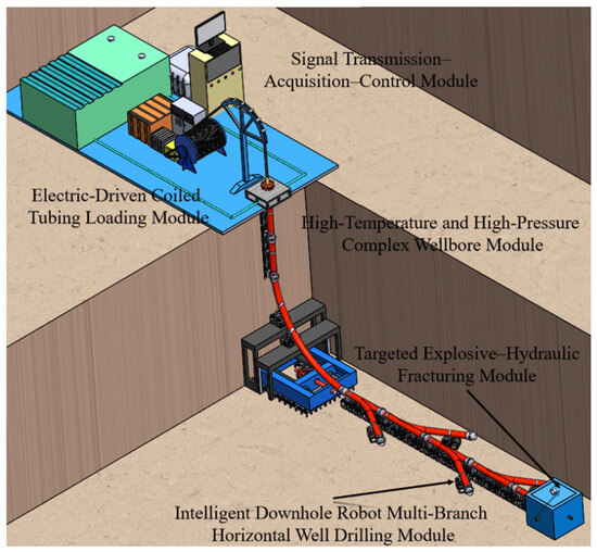
Figure 2.
Intelligent drilling and completion experimental system.
2.2.1. Hardware Section
The hardware section consists of an electrically driven coiled tubing loading module, a simulated wellbore module, a large-scale downhole core sample loading module, and other auxiliary facilities.
Electrically driven coiled tubing loading module: This serves as the power unit for the tubular string. It includes a fluid supply system that provides high-pressure workover fluid for drilling and fracturing. The supply system operates in coordination with rollers, guides, an injector head, and a wellhead device to simulate the deployment and retrieval of coiled tubing inside the wellbore.
Simulated wellbore module: This module consists of vertical, curved, and horizontal sections, constructed using 51/2″ and 95/8″ casings, flanges, and cross joints. The wellbore provides the operating environment and hardware conditions for functional modules, serves as the carrier for the layout of transmission devices within the control system, and forms the main pathway for data acquisition and transmission. It also functions as a connection module, linking the surface coiled tubing loading module with the downhole large-scale core loading module, and can simulate drilling environments under different pressure and temperature conditions.
Large-scale downhole core sample loading module: This module is designed for robotic drilling and combined explosive-hydraulic fracturing processes. It accommodates cubic rock samples ranging from 600 mm to 800 mm, and is equipped with acoustic emission probes to monitor the fracturing process while simulating high-temperature and high-pressure reservoir conditions.
2.2.2. Functional Module
The functional module consists of two main parts: the drilling assembly module and the downhole robot module.
- (1)
- Drilling assembly module: This module comprises an intelligent drill bit, power tools, a real-time communication device, the drilling robot, directional tools, and drill rods. Power is delivered from the surface through the electrically driven coiled tubing module, while the downhole drilling robot provides forward traction underground.
- (2)
- Downhole robot module: This module is designed to perform combined explosive–hydraulic fracturing. The traction robot drags the tubular string to deliver explosives to the branch wellbore. After the string is pulled back to a safe position, detonation is initiated, followed by hydraulic fracturing operations at the explosion site. This enables efficient fracturing of multilateral wells.
2.2.3. Transmission and Control System
The transmission and control system, also referred to as the intelligent real-time sensing and decision-making system, not only coordinates the interaction between the hardware and functional sections, but also provides real-time data acquisition in the wellbore, efficient bidirectional communication between downhole and surface, and intelligent decision-making for surface command execution.
The intelligent real-time sensing and decision-making system is composed of three subsystems: a sensing-detection subsystem, a communication subsystem, and a centralized control subsystem. The sensing-detection subsystem collects equipment parameters and transmits them to the centralized control subsystem through the communication subsystem. The centralized control subsystem makes intelligent decisions, which are then transmitted back to the hardware and functional modules via the communication subsystem.
The sensing-detection subsystem includes parameter measurement devices and sensors. Data collected by the sensors are transmitted to the centralized control subsystem through embedded gateway components and cables within the hardware section. The parameter measurement device can also transmit data wirelessly to the centralized control subsystem via a wireless communication module. The centralized control subsystem subsequently performs intelligent decision-making and sends control instructions through the communication subsystem for execution. The communication subsystem is the only pathway for two-way transmission of downhole data and surface commands. The centralized control subsystem, composed of central control software and a database, provides dynamic display of experimental system data.
2.3. Flow Field Simulation in Horizontal Branched Wellbores
Within the intelligent drilling and completion experimental system, the horizontal branched wellbore structure, due to its geometric asymmetry, annular eccentricity, and variable flow channels, often becomes the most unstable region for cuttings transport efficiency and the most prone to cuttings accumulation. Traditional experimental methods are limited by measurement capabilities and visualization constraints, making it difficult to accurately capture microscopic processes such as cuttings migration, settling, and retention inside the wellbore. Therefore, it is of great significance to apply computational fluid dynamics to simulate liquid–solid two-phase flow in branched wellbores.
Such simulation studies allow the identification of potential risk zones during the surface experimental stage, providing theoretical foundations for wellbore design and cuttings transport strategies in complex multilateral wells during field operations. Consequently, conducting flow field simulations of cuttings transport in branched wellbores within this experimental system framework not only enhances the completeness of the system’s functions, but also contributes theoretical models and optimization pathways for the advancement of intelligent drilling and completion technologies under realistic operating conditions.
3. Numerical Simulation Model
3.1. Mathematical Model
In this study, the liquid–solid two-phase flow is described using the Eulerian–Eulerian two-fluid model, combined with the kinetic theory of granular flow [20], to account for the interactions between drilling fluid and cuttings particles. The governing equations include the continuity equation, momentum conservation equation, and energy conservation equation.
3.1.1. Continuity Equations
The liquid-phase continuity equation reflects the fundamental principle of local mass conservation during the liquid flow process. In other words, the rate of change in liquid mass per unit volume equals the net mass flux through the control surface. It can be expressed as follows:
where is the liquid volume fraction, %; is the liquid density, kg/m3; and is the liquid velocity vector, m/s.
The solid-phase continuity equation describes the conservation of mass for the solid phase within the flow system. It is analogous to the liquid-phase continuity equation, indicating that the solid mass cannot be created or lost within the control volume. The expression is as follows:
where is the solid volume fraction ( + = 1), %; is the solid density, kg/m3; and is the solid velocity vector, m/s.
3.1.2. Momentum Equations
The liquid-phase momentum equation describes that during the flow process, the rate of change in momentum per unit volume of liquid originates from the pressure gradient, and the viscous stress within the liquid, gravitational forces, and the interactions between liquid and solid particles. In other words, it illustrates the motion behavior of the liquid phase under the influence of these forces, and is expressed as follows:
where p is the pressure, N/m2; τₗ is the liquid stress tensor, Pa; g is the gravitational acceleration vector, m/s2; is the interaction force between the liquid and solid phases, N/m3; is the molecular viscosity, Pa·s; is the turbulent viscosity, Pa·s.
The solid-phase momentum equation describes that within the flow system, the rate of change in momentum per unit volume of particles originates from the pressure exerted by the fluid, particle–particle stress, gravitational forces, and the action of the fluid on the particles. In other words, it represents the motion behavior of solid particles under the combined action of various forces in the liquid environment, and can be written as follows:
where is the solid stress tensor, Pa; is the interaction force of the liquid phase on the solid phase ( = −, the interaction forces between the two phases follow Newton’s third law), N/m3; is the solid pressure, Pa.
3.1.3. Stress Tensor Equations
The liquid-phase stress tensor is expressed as follows:
where
The solid-phase stress tensor is given as follows:
where
where I is the unit tensor, N/m2; is the solid shear stress tensor, N/m2; is the granular temperature (a measure of particle kinetic energy), m2/s2; e is the coefficient of restitution for particle collisions; is the total solid shear viscosity, Pa·s.
3.1.4. Solid Shear Stress Model
The solid-phase shear viscosity equation is used to characterize the ability of the solid particle layer to resist shear deformation during flow. Its core concept is the momentum exchange and drag interactions between particles. This equation decomposes the solid-phase viscosity into three physical mechanisms: the collisional contribution, which represents the momentum transfer during short-time elastic collisions of particles; the kinetic contribution, which denotes the shear effect caused by the free motion of particles in dilute regions; the frictional contribution, which describes the shear resistance induced by continuous contacts among particles in dense regions. The expression is given as follows [29,30]:
where
where is the collisional shear viscosity, Pa·s; is the kinetic shear viscosity, Pa·s; is the frictional shear viscosity, Pa·s; is the particle diameter, m; is the radial distribution function; is the internal friction angle, rad; is the local shear rate, 1/s; is the critical concentration.
3.1.5. Liquid–Solid Interphase Drag Model
In the Euler–Euler model, the momentum exchange between the liquid and solid phases is represented by a drag force source term . The choice of the drag coefficient directly affects the prediction of particle acceleration, settling, and pressure drop. In this study, a hybrid drag model combining the Gidaspow model [31], Ergun model [32], and Wen-Yu model [33] is adopted. The governing equations are as follows:
when >0.2 (dense regime):
when ≤0.2 (dilute regime):
where the drag coefficient is given by [34]
and the particle Reynolds number is defined as
where is the interphase drag coefficient, kg/m3·s; is the particle drag coefficient [34]; is the particle Reynolds number.
3.2. Geometric Model
In this study, a three-dimensional horizontal wellbore structure based on a Cartesian coordinate system was established using SOLIDWORKS 2025 software (version 33.0.0.5050) to simulate the transport behavior of drilling fluid carrying cuttings within the wellbore. The inlet, outlet, and flow direction of the drilling fluid are shown in Figure 3.
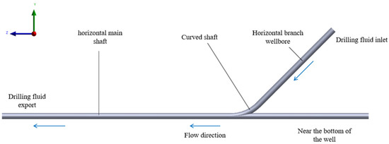
Figure 3.
Schematic of the horizontal branched wellbore model.
The horizontal branched wellbore consists of a section of horizontal main wellbore, a branched wellbore, and a curved section connecting them. The figure presents a top view, with the coordinate system established with the center point of the main wellbore outlet as the origin. The X-axis is defined as the vertical direction, with the negative direction pointing toward gravity (vertically downward) and the positive direction pointing vertically upward, representing the buoyancy direction of the fluid.
The Y-axis is defined as the direction in the horizontal plane perpendicular to the Z-axis, which corresponds to the normal expansion direction of the drilling fluid entering from the branched wellbore. The Z-axis is defined as the extension direction of the main wellbore in the horizontal plane, with the positive direction of the Z-axis representing the main flow path of the drilling fluid, as shown in Figure 3.
The drilling fluid enters the system from the right-hand side of the figure, flowing along the Z–Y plane in a curved manner and ultimately exiting the system in the positive direction of the Z-axis at the main wellbore outlet. The geometric relationships between the branched wellbore, curved wellbore, and horizontal main wellbore are defined according to this coordinate system.
The length of the main wellbore is set to 5000 mm, and the length of the branched wellbore is 2300 mm, with an angle of 45° corresponding to the curve to better simulate the flow diversion characteristics in the branched wellbore structure. The model has simplified the structure of the wellbore wall and joints for simplicity and reduced the influence of small-scale boundary movements.
In this paper, a comprehensive consideration of both the calculation resources and the practical situation of the wellbore model is taken. The model parameters used are shown in Table 1.

Table 1.
Simulation parameters.
As shown in Figure 4, when performing mesh generation using ANSYS Fluent 2024 R2 Meshing software (version 24.2.0.3796), the structural particularities and detailed features must be fully considered. Due to the complex internal flow structure of the wellbore, with local curvature changes and eccentric narrow gap regions, a hybrid mesh strategy combining structured and unstructured grids is used to improve simulation accuracy and computational stability.
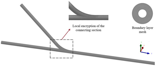
Figure 4.
Grid division of the model.
The main wellbore and the branched wellbore are meshed using hexahedral grid combinations, while the curved sections use unstructured grids with local refinement. The outer and inner walls are treated with expansion, and the mesh growth rate is set to 1.2 to ensure overall mesh accuracy.
3.3. Grid Independence Analysis
To minimize the influence of mesh quantity on the simulation results and accurately capture the reverse circulation behavior and cuttings transport characteristics within the branched horizontal wellbore, a wellbore model with an outer diameter of 139.7 mm, an eccentricity of 0%, and a curvature of 2°/30 m was selected for mesh independence verification.
The average pressure at the cross-section connecting the horizontal and curved sections is used as the evaluation parameter. Figure 5 presents the pressure variation curves obtained under different mesh densities. As shown in Figure 5, the simulated pressure values gradually stabilize as the number of cells increases. When the mesh count exceeds 500,000, the average cell size is 0.1 m, while the average cell size in the locally refined regions is 0.01 m. Further refinement yields negligible improvement in accuracy. Therefore, a mesh size of approximately 500,000 elements was adopted for the numerical simulations in this study.
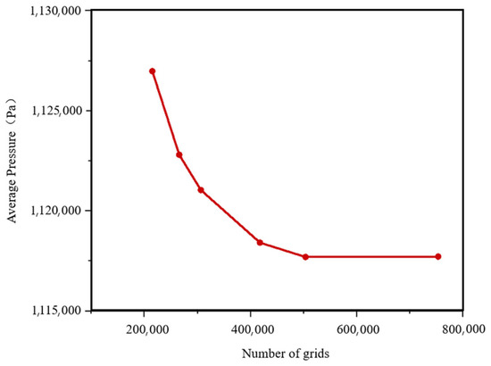
Figure 5.
Pressure drop curves under different grid numbers.
3.4. Boundary Conditions
In the numerical simulation conducted using ANSYS Fluent 2024 R2, software (24.2.0.3796) the wall boundary was set as a fixed no-slip condition with the standard wall function model applied. The turbulence model adopted is the RNG k-ε model, which converges faster than the standard k-ε model and is more effective in analyzing turbulent flows with high strain rates and pronounced curvature [35]. For the discretization of convection terms, the second-order upwind scheme is used due to its higher accuracy and suitability for complex fluid–structure coupling scenarios [36]. The SIMPLE pressure–velocity coupling algorithm, a pressure-based segregated approach, is employed for the solution process, as it is well suited for low-speed, incompressible flows and has demonstrated strong performance in complex problems such as combustion and multiphase flow [37].
At the computational domain inlet, the boundary condition is defined as a velocity inlet, with the liquid phase inlet velocity set to 2.8 m/s and the solid phase inlet velocity set to be identical to that of the liquid phase. At the outlet, a pressure outlet boundary condition is applied, with the pressure specified as 1 MPa. To better match field conditions, the Euler–Euler two-fluid model is adopted, in which both the solid and liquid phases are treated as pseudo-continuous media that exist independently yet interpenetrate with each other.
4. Transient Simulation Analysis
To further verify the accuracy of the simulation in depicting the transport of cuttings in the horizontal wellbore under actual operating conditions, this section conducts a transient simulation to analyze the dynamic behavior of cuttings transport over time. The goal is to study the transient transport characteristics of cuttings and identify any deviations in the flow pattern over time, based on real-world operational conditions. This analysis not only captures the transient characteristics of cuttings movement but also helps optimize the management of such transport behaviors during well operations.
4.1. Simulation Parameters and Boundary Conditions
The model setup for the transient simulations follows the same basic parameters used in the previous steady-state models. The wellbore geometry consists of a main wellbore with a diameter of 139.7 mm, an eccentricity of 0%, and a curvature of 2°/30 m. The drilling fluid flow rate is set to 30 L/s, with a total length of 5000 mm for the wellbore, and the mesh is refined to ensure precision in the transient simulation. The grid size is selected to be approximately 500,000 cells to ensure that the results reflect realistic fluid behavior and cuttings transport in the wellbore, considering the complexities of both the geometry and the transient flow conditions.
4.2. Transient Process Results
The transient simulation results of the cuttings volume fraction distribution are shown in Figure 6, where cuttings are primarily deposited near the bottom end of the main wellbore. As illustrated in Figure 7, when viewed from a bottom-up perspective, the transient simulation reveals the dynamic behavior of cuttings transport. It can be clearly observed that as the drilling fluid flows from the horizontal branch wellbore into the main wellbore, a noticeable backflow occurs at the junction between the curved and main sections. This backflow causes part of the cuttings to be carried and subsequently deposited at the lower region near the bottom end of the main wellbore.
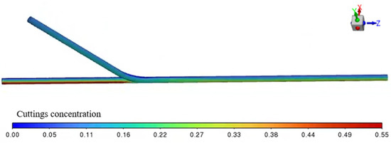
Figure 6.
Transient simulation results of cuttings volume fraction cloud diagram.
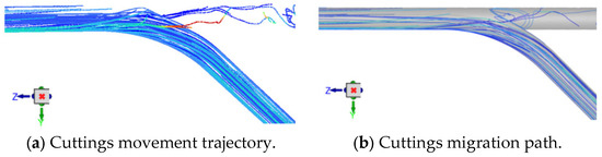
Figure 7.
Transient simulation of cuttings transport.
Through the analysis of the temporal evolution of particle volume fraction, the transient simulation clearly reveals the overall migration path and time-dependent characteristics of the cuttings. As shown in Figure 8, at the early stage of 5 s, particles are carried into the annulus by the drilling fluid flowing through the horizontal branch wellbore. The overall concentration of cuttings within the wellbore is relatively low, and although most particles gradually settle at the bottom of the main wellbore and near its lower end, the variation in concentration along the wellbore remains minor.
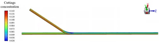
Figure 8.
Cuttings distribution cloud map at 5 s.
As shown in Figure 9, when the simulation time reaches 10 s, cuttings begin to aggregate and deposit noticeably at the junction between the branch and main wellbores. Local fluid disturbances induce partial recirculation zones, causing particles to swirl and accumulate in these regions. By 20 s, as illustrated in Figure 10, the continuous buildup of cuttings and the persistent backflow near the connection section led to gradual deposition along the lower part of the main wellbore, especially near its bottom end, where cuttings accumulation becomes more pronounced.
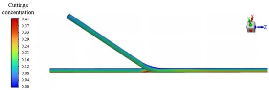
Figure 9.
Cuttings distribution cloud map at 10 s.
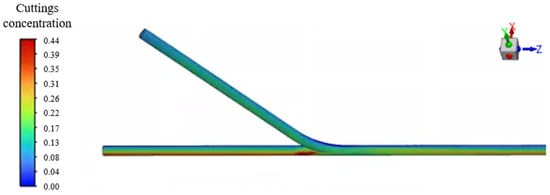
Figure 10.
Cuttings distribution cloud map at 20 s.
As shown in Figure 11, at the later stage of 50 s, the particle volume fraction field gradually reaches a stable state. Some particles are carried by the drilling fluid into the main wellbore and settle along its lower section, while most particles accumulate near the bottom end of the main wellbore where the local flow velocity is extremely low. During the backflow induced in the curved section, these particles gradually migrate backward and ultimately concentrate at the bottom of the main wellbore near its lower end.

Figure 11.
Cuttings distribution cloud map at 50 s.
4.3. Comparison with Steady-State Simulation Results
The results of the transient simulation are consistent with previous studies [38]. To verify the accuracy of the steady-state simulation results, the volume fraction field obtained from the later stage of the transient simulation is compared with the results from the steady-state calculation. It is found that both results showed similar particle accumulation areas, sedimentation trends, and distribution patterns, indicating that the steady-state results demonstrate good convergence and representativeness in terms of particle transport characteristics. The transient simulation, however, dynamically revealed the particle deposition process, which enhanced the physical plausibility of the steady-state calculations.
The transient simulation introduced in this section effectively supplements the time-evolution process of cuttings transport, validating the reliability of the particle distribution results from the steady-state calculation. Particularly in the junction area of the branched wellbore, the particle accumulation and sedimentation process further supports the credibility of the steady-state simulation results. This transient analysis provides an important dynamic foundation for subsequent comparisons and optimization under different operating conditions.
5. Influencing Factors on Cuttings Transport in the Annulus
5.1. Effect of Wellbore Diameter
Under the conditions of an eccentricity of 0%, a branch well curvature of 2°/30 m, a flow rate of 30 L/s, a consistency index k = 0.5 Pa·sn, and a flow behavior index n = 0.6, simulations were conducted by varying the wellbore outer diameter to investigate its influence on cuttings transport behavior. In the model, Position 1 is located 2 m from the drilling fluid outlet, Position 2 is 5 m from the outlet at the junction between the curved and straight sections, Position 3 is at the junction between the branch and curved sections, and Position 4 is 6.5 m from the outlet near the lower end of the main wellbore. These positions are presented in Figure 12.
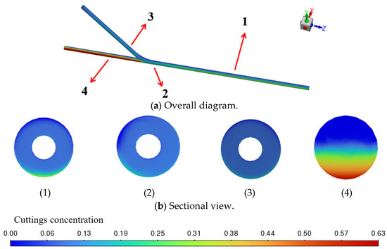
Figure 12.
Cuttings volume fraction cloud map with wellbore diameter of 139.7 mm.
Figure 12 shows the cuttings volume fraction distribution when the wellbore outer diameter is 139.7 mm. As illustrated in Figure 12a, the cuttings are relatively uniformly distributed within the annulus, and apart from the region near the lower end of the main wellbore, no significant accumulation occurs elsewhere, indicating that the drilling fluid exhibits strong cuttings-carrying capability under this diameter condition. At Position 2, the average cuttings concentration is 10.01%, which is relatively low, forming a continuous and stable low-concentration zone that reflects effective local transport by the flow field. In contrast, at Position 4, a distinct high-concentration deposition band appears, concentrated in the lower section of the wellbore, with an average concentration as high as 17.94%, indicating severe cuttings accumulation in this confined region.
Figure 13 presents the cuttings volume fraction distribution for a wellbore with an outer diameter of 177.8 mm. As shown in Figure 13a, the overall cuttings concentration distribution is more complex than that in Figure 12a, with noticeably higher concentrations appearing in the curved and confluence regions. At Position 2, the average cuttings concentration reaches 10.17%, indicating that as the outer diameter increases, the local fluid’s ability to suspend cuttings weakens, making the particles more prone to retention. At Position 4, although significant deposition remains, the overall concentration decreases to 14.81%, and the extent of high-concentration regions becomes smaller than that in Figure 12. This demonstrates that a larger wellbore diameter helps to disperse the local flow field, thereby alleviating cuttings accumulation near the lower end of the main wellbore.
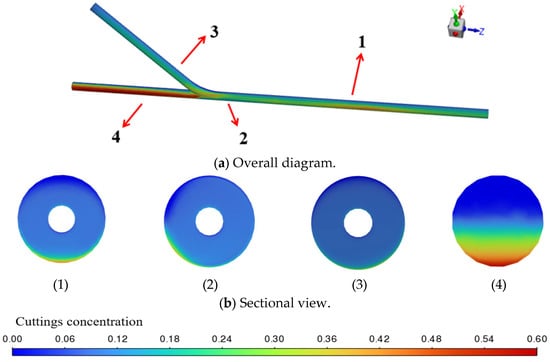
Figure 13.
Cuttings volume fraction cloud map with wellbore diameter of 177.8 mm.
Figure 14 shows the cuttings volume fraction cloud plot for a wellbore diameter of 244.5 mm. As shown in Figure 14a, the overall color is darker, with high-concentration distributions observed in most areas of the wellbore. This indicates that as the wellbore diameter further increases, cuttings are more likely to accumulate within the annular region. At location 2, the average concentration rises to 10.28%, and the red-orange regions expand further, demonstrating a continued decrease in the fluid’s ability to carry the cuttings. However, at location 4, the extent of cuttings deposition is significantly reduced compared to the previous two cases. The average concentration decreases to 12.65%, and the cloud plot shows that the low-concentration region expands, indicating that the fluid’s diffusion effect effectively dispersed the local cuttings accumulation.
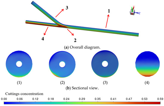
Figure 14.
Cuttings volume fraction cloud map with wellbore diameter of 244.5 mm.
Based on the results shown in Figure 12, Figure 13 and Figure 14, the influence of wellbore outer diameter on cuttings transport exhibits a dual characteristic. In most regions of the annulus, except near the lower end of the main wellbore, the cuttings concentration increases with larger diameters, indicating a gradual decline in cuttings-carrying efficiency. Conversely, at the lower end of the main wellbore, an increase in outer diameter helps reduce local cuttings concentration, thereby alleviating deposition.
Overall, the maximum cuttings concentration decreases as the wellbore diameter increases. Smaller diameters are more effective in maintaining clean flow within the branch, curved, and straight sections, while larger diameters are advantageous for mitigating accumulation near the bottom of the main wellbore. This suggests that the design of the wellbore diameter should balance cuttings transport characteristics across different regions.
5.2. Effect of Eccentricity
Under the conditions of a wellbore outer diameter of 139.7 mm, a branch well curvature of 2°/30 m, a flow rate of 30 L/s, a consistency index k = 0.5 Pa·sn, and a flow behavior index n = 0.6, simulations were conducted by varying the eccentricity to investigate its influence on cuttings transport behavior. Figure 15, Figure 16 and Figure 17, respectively, illustrate the cuttings volume fraction distributions under different eccentricities, the cross-sectional volume fraction profiles at various distances from the drilling fluid outlet, and the corresponding velocity field distributions.
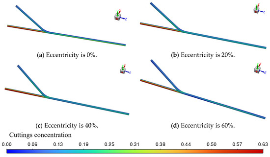
Figure 15.
Cuttings volume fraction cloud maps under different eccentricities.
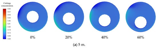
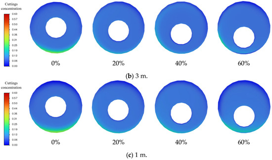
Figure 16.
Cross-sectional cuttings concentration cloud maps under different eccentricities.
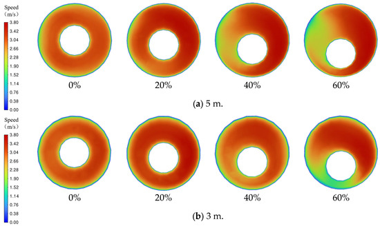

Figure 17.
Cross-sectional flow velocity cloud maps under different eccentricities.
As shown in Figure 15, when the eccentricity is 0%, cuttings are uniformly distributed along the lower section of the main wellbore, with an overall low concentration, and deposition occurs mainly at the bottom near the lower end of the main wellbore. As the eccentricity increases to 20%, 40%, and 60%, cuttings progressively migrate toward the lower side of the annulus, showing a clear accumulation trend. At higher eccentricities, localized regions of elevated concentration appear in the lower annulus, forming distinct zones prone to cuttings deposition. Moreover, with increasing eccentricity, both the local concentration near the bottom of the main wellbore and the overall maximum cuttings volume fraction rise significantly.
Three typical cross-sections at distances of 1 m, 3 m, and 5 m from the main wellbore outlet are extracted to compare the cuttings volume fraction and transport velocity distributions under different eccentricity conditions, as shown in Figure 16 and Figure 17. The perspective in the figures is from the main wellbore outlet, looking inward along the centerline direction of the wellbore, with the cross-sectional plane perpendicular to the main wellbore axis.
From the cuttings volume fraction cloud maps in Figure 16a–c, it can be observed that at 5 m, where the branched wellbore connects to the main wellbore, the drilling fluid carrying cuttings enters the main wellbore from the positive half of the Y-axis. As a result, the cuttings concentration near the branched wellbore side is significantly higher than on the side far from the branched wellbore. As the drilling fluid transports the cuttings from 5 m to 3 m and 1 m, the distribution of the cuttings concentration gradually returns to a more typical pattern, with the bottom concentration being notably higher than at the upper part.
As the eccentricity increases, the degree of cuttings deposition in the lower annulus progressively intensifies, especially at 1 m, where the effect is most pronounced. At 60% eccentricity, a significant accumulation of cuttings is observed at the bottom of the wellbore, forming a crescent-shaped high-concentration sedimentation zone, with the volume fraction peak being significantly higher than at lower eccentricities. Overall, increasing eccentricity significantly enhances the asymmetry of the annular space, leading to an uneven distribution of cuttings in the cross-section, thereby reducing the efficiency of cuttings transport.
Correspondingly, the cuttings transport velocity cloud plots at different locations shown in Figure 17 demonstrate that eccentricity also has a significant impact on the velocity distribution. At 5 m, where the branched wellbore connects to the main wellbore, the velocity near the branched wellbore is significantly lower than that far from the branched wellbore. As eccentricity increases, this trend becomes more pronounced. From the velocity cross-sectional cloud plots at 5 m, 3 m, and 1 m from the outlet, it can be observed that the cuttings transport velocity in the lower annular region near the wellbore wall decreases significantly, and the high-velocity region gradually shifts upward in the wellbore, showing a distinct shift in the flow field.
This asymmetric change in velocity distribution exacerbates the unevenness of cuttings deposition, especially by creating a stagnation zone in the lower part where the velocity is extremely low, further promoting cuttings accumulation and deposition in this region.
In summary, the higher the eccentricity is, the more apparent the instability of cuttings transport in the annulus is. Increased eccentricity intensifies the velocity asymmetry, reinforcing the deposition mechanism, making it one of the key factors affecting cuttings deposition. The higher the eccentricity, the more severe the cuttings deposition in the lower wellbore, with higher concentration and lower velocity, leading to reduced cuttings transport efficiency.
5.3. Influence of Branch Wellbore Curvature
Keeping all other parameters constant, the wellbore outer diameter of 139.7 mm, eccentricity of 0%, a flow rate of 30 L/s, a consistency index k = 0.5 Pa·sn, and a flow behavior index n = 0.6. This section investigates the influence of branch wellbore curvature on cuttings transport characteristics. The branch curvature was set to 1.5°/30 m, 2°/30 m, 2.5°/30 m, and 3°/30 m, corresponding to curvature radii of 1145.92 mm, 859.44 mm, 687.55 mm, and 572.96 mm, respectively.
As shown in Figure 18, the cuttings volume fraction distributions and corresponding average value curves at a cross-section located 6 m from the main wellbore outlet (i.e., near the lower end of the main wellbore) reveal that the cuttings accumulation area in the middle of the cross-section gradually expands with increasing curvature. The cuttings volume fraction also rises, and the overall distribution becomes less uniform. When the curvature is 1.5°/30 m, cuttings mainly concentrate in the lower region of the wellbore, with relatively low volume fractions. As the curvature increases to 3°/30 m, the average cuttings volume fraction rises from approximately 14.8% to 15.9%, indicating that greater curvature significantly enhances particle settling near the bottom of the main wellbore.
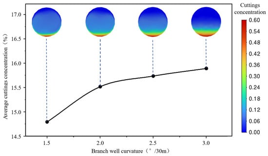
Figure 18.
Cuttings volume fraction distribution curves under different branch wellbore curvatures.
This behavior can be attributed to the intensified bending of the fluid flow path caused by higher curvature, which drives the cuttings downward under centrifugal force, leading to a distinct accumulation layer near the bottom. Moreover, larger curvature results in stronger flow disturbances at the junction between the branch and main wellbores, further promoting particle enrichment in the lower region.
To further analyze the variation trend of cuttings transport capacity, Figure 19 presents the annular velocity distribution contours and corresponding average velocity curves at the junction between the branch and main wellbores under different curvature conditions. The results indicate that as the wellbore curvature increases, the overall flow velocity at the junction slightly rises, with the cross-sectional average velocity increasing from 2.794 m/s to 2.808 m/s. This demonstrates that greater curvature intensifies local flow velocity and strengthens the flow field.
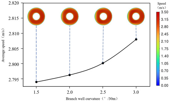
Figure 19.
Annular velocity distribution under different branch wellbore curvatures.
The increase in velocity can be attributed, on one hand, to the enhanced inertial effects and pressure drop within the curved section, and on the other hand, to the improved local cuttings-carrying capacity induced by the strengthened flow. However, since the cuttings’ particle size and density remain constant and the flow rate is unchanged, the elevated local velocity cannot effectively remove deposited particles from low-velocity regions. Consequently, the overall cuttings concentration increases despite the localized flow intensification.
Therefore, it can be concluded that increasing the curvature of the branch wellbore enhances local flow disturbances and velocity but does not effectively improve the overall cuttings-carrying performance. On the contrary, the curved geometry promotes greater particle retention in the lower part of the junction section, thereby intensifying the risk of accumulation near the lower end of the main wellbore.
This finding provides important insight for the optimization of branch wellbore design, suggesting that the curvature of the branch section should be carefully controlled to balance directional performance and flow stability. Maintaining a moderate curvature is recommended to reduce cuttings accumulation and minimize the risk of blockage in the junction and near-bottom regions.
In branch wells, flow disturbances at junctions and curved sections induce local recirculation and vortices, causing transient cuttings retention and release. This leads to deviations between downstream concentration measurements and actual transport efficiency. The mechanism is analogous to the wellbore storage effect in transient pressure analysis, where temporary fluid storage causes signal delay and distortion. Similarly, the junction region acts as a “cuttings storage unit”, introducing phase lag and filtering effects that may result in the apparent misjudgment of transport efficiency.
5.4. Influence of Flow Rate
With other conditions kept constant, including a wellbore diameter of 139.7 mm, eccentricity of 0%, branch wellbore curvature of 2°/30 m, consistency index k = 0.5 Pa·sn, and flow behavior index n = 0.6, this section investigates the effect of different flow rates on cuttings transport in horizontal branch wellbores. Four flow rates were considered: 25 L/s, 30 L/s, 35 L/s, and 40 L/s. The analysis focuses on variations in the cuttings volume fraction distribution along radial positions at the outlet, the concentration distribution at the cross-section of the branch and main wellbore junction, and the evolution of the annular velocity field.
As shown in Figure 20, within the 0~5 m section of the main wellbore, the cuttings concentration exhibits a slightly decreasing trend with increasing radial distance from the outlet, regardless of the flow rate. Overall, larger flow rates correspond to lower average cuttings concentrations in this region. At 5 m, corresponding to the junction between the curved and straight wellbore sections, a sharp increase in cuttings volume fraction is observed, indicating that this location is a critical area prone to plugging, where cuttings tend to accumulate. In the 5~8 m range, corresponding to the lower end of the main wellbore, the cuttings concentration increases progressively with distance from the outlet. Unlike the upstream section, this region shows the opposite trend: as the flow rate increases, the average cuttings concentration also rises, suggesting that higher flow rates intensify recirculation and promote particle deposition near the wellbore bottom.
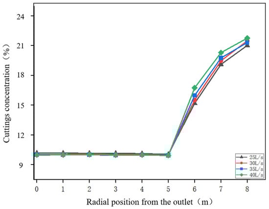
Figure 20.
Cuttings volume fraction curves under different flow rates.
From the cuttings concentration contour maps at the junction of the curved and straight wellbore sections under different flow rates shown in Figure 21, it can be observed that increasing the flow rate significantly alleviates cuttings accumulation in the lower part of the wellbore. The cross-sectional average cuttings volume fractions at flow rates of 25 L/s, 30 L/s, 35 L/s, and 40 L/s are 10.04867%, 10.00945%, 9.993403%, and 9.967008%, respectively. Although the overall reduction in average concentration is relatively small, the area of high-concentration regions decreases and the concentration gradient becomes smoother with higher flow rates, indicating an improved cuttings transport effect. In particular, at 35 L/s and 40 L/s, the cuttings distribution is more uniform and the overall concentration is reduced, demonstrating the enhanced carrying efficiency at larger flow rates.
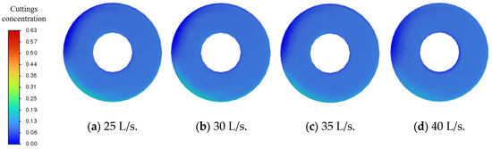
Figure 21.
Cuttings volume fraction cloud maps under different flow rates.
Further analysis of Figure 22 shows that increasing the flow rate markedly elevates the annular velocity at the junction, with the cross-sectional average rising from 2.33 m/s to 3.73 m/s. The velocity contours also indicate a pronounced shrinkage of low-velocity zones and a more uniform velocity distribution across the section. While higher velocities enhance momentum transfer and help sweep cuttings out of low-speed deposition regions, thereby reducing the likelihood of settling, high flow rates simultaneously intensify recirculation. As a result, despite improved cleaning of the upstream main wellbore, cuttings accumulation near the lower end of the main wellbore increases, leading to a higher local concentration in that region.
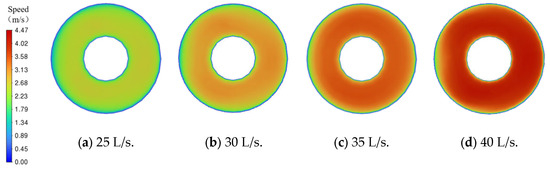
Figure 22.
Annular velocity cloud maps under different flow rates.
Based on the above analysis, under the present experimental conditions and model settings, increasing the drilling fluid flow rate effectively enhances the flow field strength and the cuttings-carrying capacity in the main wellbore section, suppressing particle accumulation at the junction and improving the overall cuttings transport performance in complex wellbore geometries. This enhancement contributes to higher hole-cleaning efficiency. However, in the lower end region of the main wellbore, the intensified recirculation associated with higher flow rates leads to an unexpected rise in the average cuttings concentration, resulting in more severe particle deposition along the wellbore bottom.
5.5. Influence of Rheological Parameters (k–n Values)
With other conditions kept constant, including a wellbore diameter of 139.7 mm, eccentricity of 0%, branch wellbore curvature of 2°/30 m, and flow rate of 30 L/s, this section further analyzes the influence of non-Newtonian fluid rheological parameters on cuttings transport within the wellbore. Figure 23 illustrates the effects of different flow behavior indices (n) on cuttings concentration, pressure, and velocity at 5 m from the drilling fluid outlet, corresponding to the junction between the branch and main wellbores, under the fixed condition of a consistency index (k) of 0.5 Pa·sn.

Figure 23.
Variation in parameters with flow behavior index.
As n increases from 0.4 to 0.8, the average cuttings volume fraction rises from 9.96% to 10.08%, showing a gradual upward trend, which indicates that as the shear-thinning property of the fluid weakens, cuttings in the annulus are more easily suspended and carried. Meanwhile, the wellbore pressure increases from 1,010,894 Pa to 1,042,880 Pa, reflecting a significant rise in pressure drop. The average velocity, however, decreases slightly from 2.801 m/s to 2.794 m/s. These results suggest that a larger flow behavior index enhances cuttings-carrying capacity, but at the expense of higher-pressure losses and a slight reduction in velocity.
Figure 24 presents the influence of different consistency indices (k) on cuttings transport in the wellbore under the fixed condition of a flow behavior index (n) of 0.6. As k increases from 0.2 Pa·sn to 0.8 Pa·sn, the average cuttings volume fraction gradually decreases from 10.13% to 9.99%. This indicates that a larger consistency index enhances the overall viscosity of the fluid, leading to a more uniform and stable distribution of cuttings, but at the expense of reduced suspension capacity. Meanwhile, the wellbore pressure rises significantly from 1,011,539 Pa to 1,022,134 Pa, reflecting a marked increase in flow resistance with higher k. The average velocity decreases slightly from 2.797 m/s to 2.795 m/s, showing only a minor change but with a clear downward trend.
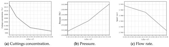
Figure 24.
Variation in parameters with consistency index.
In summary, the rheological parameters of non-Newtonian fluids exert a significant influence on the cuttings transport process. An increase in the flow behavior index (n) enhances the suspension and carrying capacity of cuttings but leads to greater annular pressure drops. Conversely, an increase in the consistency index (k) primarily manifests as elevated flow resistance and suppressed velocity, while the cuttings volume fraction shows a slight decrease.
6. Experimental Validation
6.1. Experimental Setup
To verify the rationality and reliability of the cuttings transport obtained from numerical simulations, a small-scale visualized experimental apparatus was constructed, as shown in Figure 25. The system consists of a storage tank, transparent plastic hoses, a pumping device, and a simulated wellbore model. The simulated wellbore includes a straight section, a curved section, a branch section, and a plugging section, allowing for the direct observation of cuttings distribution and deposition in different wellbore segments. Quartz sand particles were selected as substitutes for actual drill cuttings, given their comparable size and settling characteristics. The fluid circulation was driven by a pump to ensure continuous particle movement within the wellbore, thereby maintaining stable supply and recovery of the experimental medium and reducing the influence of external conditions on the results. The power unit employed a hand-drill driven miniature pump, which drew a water and sand mixture from the storage tank into the wellbore and returned it back to the tank at the outlet, forming a closed circulation loop. The parameters of the experimental equipment and materials are shown in Table 2.
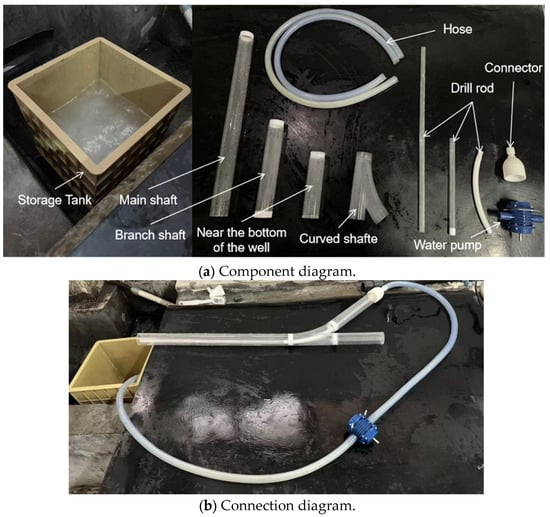
Figure 25.
Experimental setup diagram.
Table 2.
Experimental parameters of the physical model.
6.2. Experimental Procedure
6.2.1. Preparation and Assembly
During the initial preparation stage, all components required for the experiment were connected and inspected, with the fluid circulation path shown in Figure 26. All interfaces were carefully sealed, and sealing tape was applied at the joints of the simulated wellbore to prevent leakage. Clear water was then injected into the storage tank, and the water pump was operated at low speed to circulate the water through the system, entering the wellbore and flowing back to the storage tank. The system was checked for leaks, and air was expelled until no visible bubbles remained in the system. Once the setup was complete, quartz sand was mixed with clear water and stirred thoroughly to prepare a sand–water suspension with a specific volume fraction.
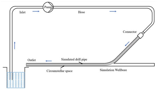
Figure 26.
Experimental pipeline setup.
6.2.2. Stable Circulation
During the experiment, the fluid in the storage tank was continuously stirred at a constant speed to ensure that the quartz sand remained uniformly suspended in the water, forming a mixture with an initial concentration of 0.1 kg/m3. The sand–water suspension was then continuously injected into the branch wellbore inlet. Driven by the pump, the sand-laden fluid entered the wellbore, gradually establishing a stable cuttings transport state. As time progressed, visual cuttings distribution and deposition patterns began to form in the curved section, main wellbore, and near the lower end of the main wellbore. Through the transparent wellbore wall, the settling and suspension of particles at different locations could be directly observed.
6.2.3. Completion and Observation
As shown in Figure 27 and Figure 28, by observing the overall wellbore as well as the localized cuttings deposition patterns at the curved section, junction, and near the lower end of the main wellbore, the distribution patterns of cuttings at different locations can be directly compared. This provides necessary experimental support and trend verification for the numerical simulation results.
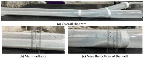
Figure 27.
Condition of rock cuttings transport at the 10th minute of the experiment.
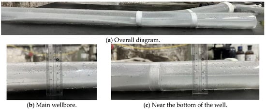
Figure 28.
Condition of rock cuttings transport at the 20th minute of the experiment.
After completing the experiment, the addition of the sand–water suspension was gradually stopped, and only clean water was circulated for a period of time to flush out any residual sand particles in the wellbore, restoring the system to a cleaner state. The residual fluid in the wellbore and piping was then drained, and the experimental setup was dismantled and organized.
6.3. Experimental Results
This experiment primarily investigates the migration and deposition evolution of cuttings under steady-state conditions. The observed results reveal a clear pattern in the spatial distribution of cuttings at different positions. As shown in Figure 27, at 10 min, the cuttings bed height in the main wellbore section (b) is approximately 1.4 cm. Although the cuttings are relatively evenly distributed along the main wellbore, the central region exhibits a noticeably higher accumulation compared to both sides. At the near-bottom end of the main wellbore (section c), the cuttings bed reaches 1.9 cm, forming a distinct “single-peak” mound with only a small amount of trailing sediment behind it. By 20 min, the cuttings bed in section (b) slightly decreases to 1.35 cm, with the central region still higher than the sides, while the near-bottom end (section c) decreases from 1.9 cm to 1.3 cm. However, the deposition pattern transitions from a localized peak to a more uniformly “spread” layer across the entire near-bottom section. This indicates that continuous fluid erosion effectively clears part of the central main wellbore, while the cuttings at the near-bottom end evolve from a concentrated pile into a thinner and more extended stable sediment layer.
Combined with the numerical simulation, the early formation of localized backflow and inertial deviation at the branch and main wellbore junction promotes the initial peak accumulation near the bottom end. As steady circulation continues, this peak gradually diminishes and diffuses downstream and laterally, forming a broader, thinner sediment layer. The experimentally measured reduction in cuttings bed height from 1.9 cm to 1.3 cm, along with the expanded coverage, together confirm that under the geometric and steady-flow conditions of a branched horizontal wellbore, cuttings continuously migrate toward and ultimately accumulate at the near-bottom section of the main wellbore. From the perspective of the deposition trend, transport pattern, and accumulation position, the experimental results show a high degree of consistency with the numerical simulation, demonstrating that the CFD model developed in this study accurately captures the fundamental mechanisms of cuttings transport in branched horizontal wellbores and validates the reliability and effectiveness of the simulation results.
7. Conclusions
Based on the intelligent drilling and completion simulation system, a three-dimensional flow field model of a branched horizontal wellbore was developed. Using the Eulerian–Eulerian two-fluid model coupled with the kinetic theory of granular flow, the effects of wellbore diameter, eccentricity, curvature, flow rate, and rheological parameters on cuttings transport were systematically investigated. The results were further validated through visualized experiments. The main conclusions are as follows:
- (1)
- Wellbore geometry strongly influences cuttings transport behavior. Increasing wellbore diameter and eccentricity intensifies cuttings deposition at the curved and junction sections, while a larger diameter helps alleviate accumulation near the lower end of the main wellbore. Greater curvature enhances local flow disturbance and centrifugal settling but reduces overall carrying efficiency, promoting particle retention in the near-bottom region.
- (2)
- Flow rate and rheological parameters significantly affect carrying capacity. Higher flow rates improve hole-cleaning performance in the main wellbore but also enhance backflow near the lower end, promoting redeposition. When the flow behavior index n increases from 0.4 to 0.8, the average cuttings concentration rises from 9.96% to 10.08% and the pressure loss increases from 1,010,894 Pa to 1,042,880 Pa, indicating enhanced transport but higher energy loss. Increasing the consistency index k raises viscosity and pressure loss, slightly reducing overall transport efficiency.
- (3)
- Experimental results show strong consistency with simulations. The measured cuttings bed height decreased from 1.9 cm to 1.3 cm, transitioning from a localized mound to a uniform layer along the near-bottom end of the main wellbore. This matches the simulated migration and deposition trends, confirming the validity and accuracy of the CFD model.
- (4)
- The combined numerical and experimental approach effectively elucidates the mechanisms of cuttings migration, deposition, and redistribution within branched horizontal wellbores, providing both theoretical guidance and experimental support for optimizing complex wellbore structures, drilling fluid design, and hole-cleaning efficiency.
Author Contributions
Conceptualization, X.W.; methodology, B.H. and X.W.; software, B.H. and X.W.; validation, Q.W. and Z.X.; formal analysis, B.H.; investigation, B.H.; resources, X.W.; data curation, Q.W.; writing—original draft, B.H. and X.W.; writing—review and editing, Q.W.; visualization, B.H. and Z.X.; supervision, X.W.; project administration, X.W. and Q.W., funding acquisition, X.W. All authors have read and agreed to the published version of the manuscript.
Funding
This work was funded by the National Natural Science Foundation of China (Grants Nos. 52204006, 52327803), the China Postdoctoral Science Foundation (Grants No. 2022M723399), and the Tianfu Yongxing Laboratory Organized Research Project Funding (Grants No. 2023KJGG13).
Data Availability Statement
The raw data supporting the conclusions of this article will be made available by the authors on request.
Acknowledgments
The authors would like to express their sincere gratitude to the Li Zhang at the Key Laboratory of Fluid and Power Machinery, Ministry of Education, Xihua University, for their assistance and discussions.
Conflicts of Interest
The authors declare no conflict of interest.
Nomenclature
| Liquid volume fraction (%) | |
| Liquid density (kg/m3) | |
| Liquid velocity vector (m/s) | |
| Solid volume fraction (, %) | |
| Solid density (kg/m3) | |
| Solid velocity vector (m/s) | |
| p | Pressure (N/m2) |
| Liquid-phase stress tensor (Pa) | |
| g | Gravitational acceleration vector (m/s2) |
| Interaction force between liquid and solid phases (N/m3) | |
| Molecular viscosity (Pa·s) | |
| Turbulent viscosity (Pa·s) | |
| Solid-phase stress tensor (Pa) | |
| Force exerted by the liquid on the solid particles (= −, consistent with Newton’s third law, N/m3) | |
| Solid-phase pressure (Pa) | |
| Effective viscosity of the liquid phase (Pa·s) | |
| Unit tensor (N/m2) | |
| Deviatoric stress tensor of the solid phase (N/m2) | |
| Θs | Granular temperature (a measure of particle kinetic energy, m2/s2) |
| e | Restitution coefficient of particle collisions |
| Total solid-phase shear viscosity (Pa·s) | |
| Collisional shear viscosity (Pa·s) | |
| Kinetic shear viscosity (Pa·s) | |
| Frictional shear viscosity (Pa·s) | |
| Particle diameter (m) | |
| Radial distribution function | |
| Internal friction angle (rad) | |
| Local shear rate (1/s) | |
| Critical solid concentration | |
| Interphase drag coefficient (kg/(m3·s)) | |
| Particle drag coefficient | |
| Particle Reynolds number |
References
- Zhuang, L. Research and application of branched well drilling technology. China Pet. Chem. Stand. Qual. 2011, 31, 77. [Google Scholar]
- Hill, A.D.; Zhu, D.; Economides, M.J. Multilateral Wells; (Translated by Zeng, X.L.); Petroleum Industry Press: Beijing, China, 2015. [Google Scholar]
- Wang, Z.; Tang, Z.; Wang, M.; Wang, A. Drilling technology of the first domestic branched horizontal well. Pet. Drill. Technol. 2001, 29, 7–9. [Google Scholar]
- Huang, D. Research and application of potential tapping technology for multilateral horizontal wells. China Well Rock Salt 2023, 54, 16–19. [Google Scholar]
- Wei, K.; Xiao, D.; Xi, C.; Wu, D.; Liao, H. Numerical simulation and analysis of holebottom pressure fluctuations during tripping operations in deep and complex wells. Phys. Fluids 2025, 37, 034105. [Google Scholar] [CrossRef]
- Hooker, P.R.; Brigham, W.E. Temperature and heat transfer along buried liquids pipelines. J. Pet. Technol. 1978, 30, 747–749. [Google Scholar] [CrossRef]
- Li, S.C. The first drilling simulation experimental device built in China. Pet. Drill. Prod. Technol. 1990, 3, 17. [Google Scholar]
- Lu, H.; Gidaspow, D.; Wang, S. Computational Fluid Dynamics and the Theory of Fluidization; Springer: Singapore, 2021. [Google Scholar]
- Cao, Y.; Li, X.; Yan, J.; Chi, Y.; Cen, K. Numerical simulation of gas–solid flow characteristics in the dense phase region of a tube-type fluidized bed. J. Zhejiang Univ. (Eng. Sci.) 2005, 39, 795–800. [Google Scholar]
- Heshamudin, N.S.K.; Katende, A.; Rashid, H.A.; Ismail, I.; Samsuri, A. Experimental investigation of the effect of drill pipe rotation on improving hole cleaning using water-based mud enriched with polypropylene beads in vertical and horizontal wellbores. J. Pet. Sci. Eng. 2019, 179, 1173–1185. [Google Scholar] [CrossRef]
- Wang, Q. Modeling and Analysis of Dynamic Cuttings Transport in Extended-Reach Wells. Master’s Thesis, Yangtze University, Jingzhou, China, 2020. [Google Scholar]
- Zhang, F.; Filippov, A.; Jia, X.; Lu, J.; Khoriakov, V. Transient solid–liquid two-phase flow modelling and its application in real-time drilling simulations. In Proceedings of the 10th North American Conference on Multiphase Technology, Banff, AB, Canada, 8–10 June 2016; pp. 17–32. [Google Scholar]
- Liu, C.W.; Li, Z.M. Research progress on cuttings transport models during drilling. Drill. Fluid Complet. Fluid 2019, 36, 663–671. [Google Scholar]
- Zhu, X.; Ling, Y.; Tong, H. Numerical simulation of gas–solid two-phase flow in air drilling with down-the-hole hammer. J. Cent. South Univ. (Sci. Technol.) 2011, 42, 3040–3047. [Google Scholar]
- Ghasemikafrudi, E.; Hashemabadi, S.H. Numerical study on cuttings transport in vertical wells with eccentric drillpipe. J. Pet. Sci. Eng. 2016, 140, 85–96. [Google Scholar] [CrossRef]
- Sun, B.; Xiang, H.; Li, H.; Li, X. Modeling of the critical deposition velocity of cuttings in an inclined slimhole annulus. SPE J. 2017, 22, 1213–1224. [Google Scholar] [CrossRef]
- Wang, Q.; Zhang, F.; Li, X.; Yang, G.; Wang, Y.; Wang, Y. Transient general solid–liquid two-phase flow model and its application in dynamic wellbore cleaning simulation. Chin. J. Appl. Mech. 2021, 38, 1044–1053. [Google Scholar]
- Zhu, X.; Shen, K.; Li, B.; Lv, Y. Cuttings transport using pulsed drilling fluid in the horizontal section of the slim-hole: An experimental and numerical simulation study. Energies 2019, 12, 3939. [Google Scholar] [CrossRef]
- Sun, S.; Feng, J.; Hou, Z.; Yu, G. Prediction of cuttings transport behavior under drill string rotation conditions in high-inclination section. Int. J. Pattern Recognit. Artif. Intell. 2020, 34, 23. [Google Scholar] [CrossRef]
- Ding, J.; Gidaspow, D. A bubbling fluidization model using kinetic theory of granular flow. AIChE J. 1990, 36, 523–538. [Google Scholar] [CrossRef]
- Xie, B.; Wang, L.; Li, H.; Huo, H.; Cui, C.; Sun, B.; Ma, Y.; Wang, J.; Yin, G.; Zuo, P. An interface-reinforced rhombohedral Prussian blue analogue in semi-solid state electrolyte for sodium-ion battery. Energy Storage Mater. 2021, 36, 99–107. [Google Scholar] [CrossRef]
- Roy, S.; Sai, P.S.T.; Jayanti, S. Numerical simulation of the hydrodynamics of a liquid–solid circulating fluidized bed. Powder Technol. 2014, 251, 61–70. [Google Scholar] [CrossRef]
- Peng, J.W.; Zhou, Q.; Geng, P.; Dong, F.; Sun, T.; Deng, W.; Li, S. Simulation analysis of wear characteristics in solid–liquid two-phase flow of high-discharge centrifugal pumps. Pet. Field Mach. 2025, 54, 44–52. [Google Scholar]
- Hu, J.; Zhang, G.; Li, J.; Chen, Y.; Yan, F. Numerical simulation of cuttings transport based on CFD–DEM coupled model. Fault-Block Oil Gas Field 2022, 29, 561–566. [Google Scholar]
- Zhu, N.; Huang, W.J.; Gao, D.L. Cuttings transport and parameter optimization for extended-reach wells under complex conditions. Pet. Mach. 2022, 50, 24–32. [Google Scholar]
- Sun, X.; Mao, N.; Ju, G.; Hu, Q.; Sun, M.; Yu, F. Cleaning efficiency of drill pipe axial movement on cuttings beds in horizontal well sections. Nat. Gas Ind. 2021, 41, 89–96. [Google Scholar]
- Ekeregbe, M.P.; Khalaf, M.S.; Samuel, R. Dull Bit Grading Using Video Intelligence. In Proceedings of the SPE Annual Technical Conference and Exhibition, Dubai, United Arab Emirates, 21–23 September 2021. [Google Scholar]
- Wang, H.; Huang, H.; Ji, G.; Chen, C.; Lv, Z.; Chen, W.; Bi, W.; Liu, L. Advances and challenges in drilling and completion technologies for deep, ultra-deep, and horizontal wells in China National Petroleum. China Pet. Explor. 2023, 28, 1–11. [Google Scholar]
- Brilliantov, N.V.; Pöschel, T. Rolling friction of a viscous sphere on a hard plane. Europhys. Lett. 1998, 42, 511. [Google Scholar] [CrossRef]
- Mathiesen, V.; Solberg, T.; Hjertager, B.H. Predictions of gas/particle flow with an Eulerian model including a realistic particle size distribution. Powder Technol. 2000, 112, 34–45. [Google Scholar] [CrossRef]
- Gidaspow, D.; Bezburuah, R.; Ding, J. Hydrodynamics of Circulating Fluidized Beds: Kinetic Theory Approach; No. CONF-920502-1; Illinois Institute of Technology: Chicago, IL, USA, 1990. [Google Scholar]
- Ergun, S. Fluid flow through packed columns. Chem. Eng. Prog. 1952, 48, 89–94. [Google Scholar]
- Wen, C.Y.; Yu, Y.H. A generalized method for predicting the minimum fluidization velocity. AIChE J. 1966, 12, 610–612. [Google Scholar] [CrossRef]
- Schiller, L.; Naumann, A. Über die grundlegenden Berechnungen beider Schwerkraftaufbereitung. Z. Des Vereines Dtsch. Ingenieure 1933, 77, 318–320. [Google Scholar]
- Hou, Q.F.; Zou, S. Comparison between standard and renormalization group k-ε models in numerical simulation of swirling flow tundish. ISIJ Int. 2005, 45, 325–330. [Google Scholar] [CrossRef]
- de Oliveira, M.; Puraca, R.C.; Carmo, B.S. A study on the influence of the numerical scheme on the accuracy of blade-resolved simulations employed to evaluate the performance of the NREL 5 MW wind turbine rotor in full scale. Energy 2023, 283, 128394. [Google Scholar] [CrossRef]
- Zhang, C.; Han, Z.; Ma, B.; Yang, Z.; Liu, Y.; Hu, Y.; Wang, Z.; Zhao, K. Coupling Changes in Pressure and Flow Velocity in Oil Pipelines Supported by Structures. Processes 2025, 13, 2932. [Google Scholar] [CrossRef]
- Wang, S.; Wang, Y.; Wang, R.; Yuan, Z.; Chen, Y.; Shao, B.; Ma, Y. Simulation study on cutting transport in a horizontal well with hydraulic pulsed jet technology. J. Pet. Sci. Eng. 2023, 224, 111429. [Google Scholar] [CrossRef]
Disclaimer/Publisher’s Note: The statements, opinions and data contained in all publications are solely those of the individual author(s) and contributor(s) and not of MDPI and/or the editor(s). MDPI and/or the editor(s) disclaim responsibility for any injury to people or property resulting from any ideas, methods, instructions or products referred to in the content. |
© 2025 by the authors. Licensee MDPI, Basel, Switzerland. This article is an open access article distributed under the terms and conditions of the Creative Commons Attribution (CC BY) license (https://creativecommons.org/licenses/by/4.0/).