A Physics-Constrained Method for the Precise Spatiotemporal Prediction of Rock-Damage Evolution

Abstract

Accurately predicting the spatiotemporal evolution of rock-damage zones is vital for underground engineering safety. Using three-dimensional data obtained from uniaxial compression–acoustic emission tests, this study addresses the key limitations of existing data-driven methods, which struggle with spatial heterogeneity and often yield predictions that deviate from fundamental fracture-mechanics principles. To overcome these challenges, we propose a physics-constrained spatiotemporal STConvLSTM framework that integrates a density-adaptive point cloud–voxel conversion mechanism for improved 3D representation, a composite loss incorporating structural and physics-based constraints, and a multi-level encoder–processor–decoder architecture enhanced by 3D convolutions, attention modules, and residual connections. Experimental results demonstrate superior accuracy and physical consistency, achieving 92.6% accuracy and an F1-score of 0.947, outperforming ConvLSTM and UNet3D baselines. The physics-aware constraints effectively suppress non-physical divergence and yield damage morphologies that better align with expected fracture-mechanics behavior. These findings show that coupling data-driven learning with physics-based regularization substantially enhances model reliability and interpretability. Overall, the proposed framework offers a robust and practical paradigm for 3D damage-evolution modeling, supporting more-dependable early-warning, stability assessment, and intelligent support-design applications in underground engineering.

1. Introduction

Accurately predicting the spatiotemporal evolution of three-dimensional rock-damage zones is fundamental for evaluating the long-term safety and durability of engineering structures. With the development of deep learning, data-driven approaches have shown strong potential in reducing prediction errors and improving computational efficiency. Meanwhile, advanced measurement techniques—LiDAR, synchrotron CT, and acoustic emission technology—provide a solid data foundation for high-precision modeling [1,2,3]. Recent studies have reported encouraging progress in areas such as deep models for surrounding-rock deformation in high-speed railway tunnels [4], hybrid constitutive modeling and deformation prediction for sandy limestone [5], transfer-learning-enhanced ConvLSTM for fracture evolution [6], LSTM-DCNN with transfer learning for mining-induced surface settlement [7], Newton–Raphson–BP prediction of rockburst intensity [8], and CNN–LSTM models under imbalanced data for rockburst grading [9]. In addition, for 3D structure learning from point cloud and voxel, VoxelNet and point–voxel fusion architectures have provided strong baselines [10,11,12], and recent surveys have systematically reviewed sparse 3D deep-learning paradigms in this field [13].

However, key bottlenecks remain for 3D damage-zone forecasting. (1) Data representation vs. fidelity: Damage point clouds are unstructured, sparse, and strongly heterogeneous; fixed-resolution voxelization easily loses details in critical areas, while pure point-based models (e.g., PointNet++) lack explicit temporal modeling [11,12]. Recent mixed point–voxel and sparse 3D backbones (PVCNN, submanifold sparse CNNs, Minkowski sparse ConvNets) markedly improve efficiency and fidelity on rock-like sparse geometries, motivating our density-adaptive voxelization design [14,15,16]. (2) Physics inconsistency: Purely data-driven predictors may generate results that deviate from fundamental fracture-mechanics principles, particularly when the training data underrepresent governing physical constraints. Physics-Informed Neural Networks (PINNs) address this issue by embedding governing PDEs as hard physical constraints, forcing the predictions to strictly satisfy mechanical laws. Phase-field and PINN-based fracture studies further demonstrate that incorporating energy-based criteria—such as Griffith-type formulations—can significantly enhance mechanical plausibility [17,18,19]. However, these hard-constraint approaches face challenges when applied to high-dimensional voxel or point cloud representations and discontinuous crack evolution, where strict PDE enforcement becomes computationally prohibitive or physically incompatible. In contrast, this study adopts a physics-constrained strategy based on soft mechanics-guided constraints, incorporating fracture-mechanics-inspired terms into the loss function to guide the model toward physically consistent damage evolution while retaining the flexibility of data-driven deep learning. This distinction between hard physics enforcement and soft physics-guided regularization is consistent with broader perspectives in physics-informed machine learning, where PINNs represent strong PDE-based constraints while alternative hybrid frameworks balance physical fidelity with data-driven flexibility [20]. (3) Spatiotemporal modeling limits: Standard ConvLSTM often relies on 2D convolutions and struggles with complex 3D topology. A 3D pathway remains essential—3D U-Net is a strong encoder–decoder baseline for volumetric context [21], and 3D-ConvLSTM has demonstrated superior forecasting of evolving volumetric structures in longitudinal medical data, motivating our 3D extension to rock-damage sequences [22].

To support the development of a reliable forecasting framework, this study builds upon the acoustic-emission-based regional correlation imaging technique proposed by Yao et al. [23] and their subsequent work on regionalized damage-structure evolution [24]. This approach enables efficient reconstruction of the initial state and dynamic point cloud sequences of three-dimensional damage zones during uniaxial compression, while related advances in 3D AE tomography and anisotropy-aware AE localization further enhance the reliability of internal imaging for rock specimens [25,26]. Motivated by the broader challenges of data heterogeneity, the need for physically consistent learning, and the modeling of complex 3D spatiotemporal patterns, this study aims to develop a deep-learning framework capable of accurately forecasting the three-dimensional evolution of rock-damage zones reconstructed from AE measurements.

The main contributions of this work are threefold. First, we design a spatiotemporal deep-learning framework tailored to sparse and evolving 3D damage representations. Second, we introduce mechanics-guided constraints to enhance physical plausibility without relying on hard PDE enforcement, thereby maintaining the flexibility of data-driven modeling. Third, we validate the proposed approach using laboratory uniaxial compression–AE data, demonstrating notable improvements in predictive accuracy, boundary fidelity, and mechanical consistency compared with conventional ConvLSTM and UNet3D baselines. These results highlight the method’s potential for early-warning, stability assessment, and intelligent support-design applications in underground engineering.

2. Materials and Methods

2.1. Data Source and Hyperparameter Setup

A time-series dataset of three-dimensional damage evolution was obtained from uniaxial compression–acoustic emission tests on rock specimens (Figure 1). The cube specimens had an edge length of 100 mm. The measurements, recorded over 18 time steps from initial damage to macroscopic failure, are stored as raw data on a 100 × 100 × 100 regular grid in .mat format. Damage regions were extracted from the velocity field using the fuzzy C-means (FCM) algorithm and converted into sequences of 3D point clouds (each record contains the velocity value and the corresponding XYZ coordinates). This dataset exhibits pronounced spatial heterogeneity and temporal evolution, making it suitable for evaluating the proposed method’s capabilities in representation, spatiotemporal modeling, and physical consistency. A sliding window with two consecutive time steps is used to construct each training sample. Specifically, the model receives the damage fields at time steps t − 1 and t as its input and learns the temporal transition reflected between these states. This learned transition is then used to estimate the damage field at the following time step t + 1. In this way, the two most recent states provide both the current condition and the immediate evolving trend required for predicting the next state.

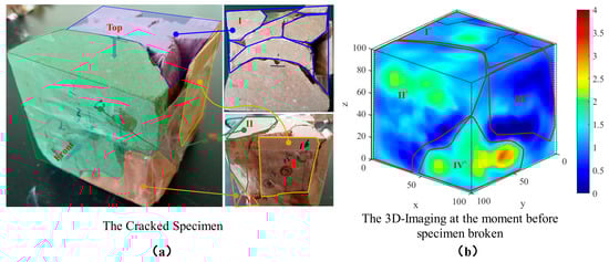
Figure 1. (a) The cracked specimen and (b) 3D imaging at the moment before the specimen is broken. The numbered regions I–IV and I*–IV* respectively denote the main fractured zones observed on the cracked specimen and their corresponding damage areas identified in the 3D imaging.

The selection of the window size 2 and other preprocessing parameters follows empirical evaluation. Several candidate configurations were tested in preliminary experiments, and the chosen values yielded the most stable prediction performance while preserving the temporal evolution pattern of the monitored damage fields. Similarly, the loss weighting coefficients listed in Table 1 were selected based on validation performance, ensuring a balanced contribution from both the data-driven and physics-guided components during training.

Table 1. Data preprocessing and training hyperparameters.

Hyperparameter	Value/Setting	Purpose
Base grid resolution for adaptive voxelization	100 × 100 × 100	Preserve spatial detail features
Input time step (sliding window)	2	Capture the recent evolutionary history
Hyperparameter	Value/Setting	Purpose
Prediction time step	1	Evaluate the accuracy of single-step predictions
Learning rate scheduling strategy	Cosine annealing	Stabilize and converge to the optimal solution
Optimizer	AdamW	Improve training stability
Composite loss weight ${\lambda }_{\mathrm{s}}$, ${\lambda }_{\mathrm{p}}$, ${\lambda }_o$	$\begin{array}{l}{\lambda }_{\mathrm{s}}=0.7\\ {\lambda }_{\mathrm{p}}=0.2\\ {\lambda }_o=0.1\end{array}$	Balance various optimization objectives

The rationale for the selected preprocessing and loss-weighting parameters is provided in Section 2.1.

2.2. Methods, Procedures, and Adaptive Voxelization

The pipeline steps are as follows: First, the global range of the dataset is analyzed, and the raw point cloud data are feature-normalized using a MinMaxScaler. Subsequently, temporal samples are constructed through a sliding-window mechanism. During the data-loading stage, adaptive voxelization based on K-nearest neighbor (KNN) density estimation accelerated by a KD-tree is performed on each time-step normalized point cloud to generate multi-resolution voxel representations. The encoder–processor–decoder STConvLSTM network with integrated CBAM3D attention modules is then employed for spatiotemporal modeling and prediction, while model parameters are optimized through a composite loss function combining structural perception loss and physical constraint loss. Finally, the predicted voxel fields are thresholded and converted back into point clouds, followed by inverse normalization to complete reconstruction and visualization evaluation.

This workflow, illustrated in Figure 2, achieves an end-to-end learning framework that synergistically integrates adaptive data representation, spatiotemporal modeling, and physical constraints, thereby substantially improving prediction accuracy while ensuring physical consistency.

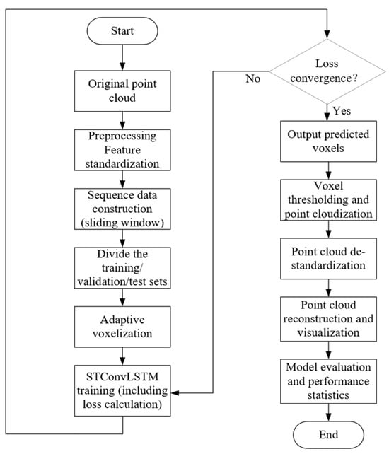
Figure 2. Method and procedures.

To enable efficient learning on regular grids while preserving critical structures, point clouds were converted to voxels via a bidirectional adaptive point cloud–voxel conversion mechanism. Local voxel granularity is dynamically adjusted according to point density: finer voxels are assigned to dense, structure-critical zones (detail preservation), whereas coarser voxels are used in sparse areas (efficiency). Figure 3 shows the adaptive voxelization process.

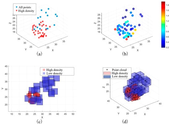
Figure 3. Adaptive voxelization process. (a) Original point cloud data. (b) Point cloud density heat map. (c) Adaptive voxelization result. (d) Comparison of point cloud and voxel data.

2.3. Physics-Constrained STConvLSTM Architecture

The network follows an encoder–processor–decoder design.

Encoder: three cascaded 3D convolutional blocks (3 × 3 × 3 kernels) with batch normalization and ReLU progressively downsample inputs into compact feature maps while increasing channels. A CBAM3D module (channel + spatial attention) is integrated after the initial feature extractor to enhance sensitivity to damage-relevant structures. CBAM3D variants have proved effective in volumetric segmentation and motivate our attention design [27,28]. Let the input voxel tensor be $V_t\in R^{C_0\times R_1\times R_1\times R_1}$, the output $E_l$ of the $l-th$ layer ($l=1,2,3$) in the encoder is computed as follows:

$$E_l=CBAM3D\left(F_l\right)$$

(1)

$$F_l=ReLU\left(BatchNorm3D\left(Conv3D_{k=3,s=n}^{\left(l\right)}\left(E_{l-1}\right)\right)\right)$$

(2)

where $E_0=V_t$ (input initialization), and $Conv3D_{k=3,s=n}^l$ denotes the 3D convolution layer of the $l$-th level with a kernel size of 3 × 3 × 3 and a stride n, which can be adjusted according to the dataset scale. In addition, the CBAM3D module in Equation (1) is further decomposed into two sequential steps—channel attention and spatial attention—as expressed by the following:

$$CBAM3D\left(F_l\right)=SpatialAtt3D\left(ChannelAtt3D\left(F_l\right)\right)$$

(3)

Here, $ChannelAtt3D\left(F_l\right)$ performs global pooling on $F_l$ followed by weighting through a multilayer perceptron (MLP), producing channel-attention weights that are multiplied with the input features. This mechanism mimics the human visual system’s selective attention to different feature channels, enabling the network to adaptively emphasize the channels relevant to rock-damage evolution while suppressing irrelevant or noisy ones. $SpatialAtt3D\left(·\right)$ then applies spatial pooling and a 7 × 7 × 7 convolution to the channel-weighted features, generating spatial-attention weights that emphasize important spatial locations. The large convolution kernel ensures a broad receptive field, effectively capturing contextual information of key structural regions in the rock-damage domain and guiding the model to focus on these spatially critical areas. Finally, $E_l$ serves as the input to the next layer, completing the effective integration of feature extraction and attention enhancement.

Spatiotemporal processor: a 3D ConvLSTM core replaces fully connected mappings with 3D convolutions in the gate transitions, enabling joint modeling in space and time and retaining path dependence of damage evolution.

Decoder: three transposed-convolution blocks (with batch normalization, ReLU, and CBAM3D) progressively restore resolution and produce the predicted damage field. The output feature of decoder can be expressed as follows:

$$D_l=CBAM3D\left(ConvTranspose3D\left(D_{l-1}\right)\right)$$

(4)

where $D_l$ denotes the output of the $l-th$ layer, and $ConvTranspose3D\left(·\right)$ represents the 3D-transposed convolution operation. To stabilize gradients and strengthen feature reuse, dual residual connections are adopted around the ConvLSTM outputs and subsequent nonlinear transforms; a lightweight spatial weighting predictor further emphasizes key regions and suppresses over-prediction at noncritical locations. The network structure is as follows (Figure 4):

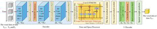
Figure 4. Network structure.

2.4. Composite Loss with Physical Constraints

The total objective combines a structure-aware term, a physics-constraint term, and an over-prediction penalty:

$$\mathrm{L}\_\mathrm{total}={\lambda }_s·\mathrm{L}\_\mathrm{structure}+{\lambda }_p·\mathrm{L}\_\mathrm{physical}+{\gamma }_o·\mathrm{L}\_\mathrm{overprediction}$$

(5)

Structure-aware loss prioritizes geometric fidelity at crack boundaries and preserves morphological continuity as follows:

$$\begin{array}{l}\mathrm{L}\_\mathrm{structure}=\alpha ·\mathrm{L}\_\mathrm{struct}+\beta ·\mathrm{L}\_\mathrm{reg}\\ \mathrm{L}\_\mathrm{struct}={\displaystyle \frac{1}{N}}{\displaystyle \sum _{i,j,k}{w}_{i,j,k}·\left|V^{pred}i,j,k-V^{t\arg et}i,j,k\right|}\\ \mathrm{L}\_\mathrm{reg}={\displaystyle \frac{1}{N}}{\displaystyle \sum _{i,j,k}\left|V^{pred}i,j,k-mean\left(V^{t\arg et}\right)\right|}\end{array}$$

(6)

where $w_{i,j,k}=1+\left|V^{pred}i,j,k-V^{t\arg et}i,j,k\right|$ represents the adaptive weight, which enables the model to pay more attention to the areas that are difficult to predict. $\mathrm{L}\_\mathrm{reg}$ maintains the structural regularity of the prediction.

The physical constraint loss is designed to incorporate classical rock mechanics theories, ensuring spatial continuity and smoothness. Specifically, the mathematical formulation of the continuity and smoothness constraints can be analogized to the Griffith energy criterion $G>2{\gamma }_s$. By constraining the spatial variation of the damage zone, the model indirectly regulates the energy release process during damage evolution. The edge-distribution constraint draws on the physical meaning of the stress intensity factor $K_I$, which suppresses abnormal distributions along the damage-zone boundaries and prevents the occurrence of a local stress concentration. Furthermore, the weighted combination of all the loss components reflects the multi-field coupling characteristics of rock materials during deformation and fracture, ensuring that the prediction results are more consistent with the actual physical mechanisms of rock failure. Based on the Griffith energy criterion, the spatial distribution of the damage zone is represented by a voxel field $V_{i,j,k}$, whose spatial variation can be approximated using finite-difference gradients as follows:

$${\left|\nabla V\right|}^2\approx {\left(V_{i+1,j,k}-V_{i,j,k}\right)}^2+{\left(V_{i,j+1,k}-V_{i,j,k}\right)}^2+{\left(V_{i,j,k+1}-V_{i,j,k}\right)}^2$$

(7)

A smaller value of this term indicates that the spatial distribution of the damage zone is more continuous and that the energy release process is smoother. The spatial stability of the energy release rate can be approximated by constraining the first- and second-order derivatives of the voxel field. Specifically, the continuity loss $L_{continuity}$ corresponds to the sum of the squares of the first-order gradients of the voxel field, reflecting the spatial continuity of the energy release process. The smoothness loss $L_{smoothness}$ corresponds to the sum of the squares of the second-order derivatives, reflecting the spatial uniformity of energy release. Their mathematical expressions are as follows:

$$L_{continuity}~{\displaystyle {\int }_{\Omega }{\left|\nabla V\right|}^2}d\Omega , L_{smoothness}~{\displaystyle {\int }_{\Omega }{\left|\Delta V\right|}^2}d\Omega$$

(8)

The physical constraint loss consists of three core components, ensuring that the predicted results conform to rock-mechanical principles:

$$\begin{array}{l}{L}_{physical}={\lambda }_c·L_{continuity}+{\lambda }_s·L_{smooth}+{\lambda }_e·L_{edge}\\ L_{continuity}={\displaystyle \frac{1}{3}}\left(E\left[\left|V_{i,j,k}-V_{i+1,j,k}\right|\right]+E\left[\left|V_{i,j,k}-V_{i,j+1,k}\right|\right]+E\left[\left|V_{i,j,k}-V_{i,j,k+1}\right|\right]\right)\\ L_{smoothness}={\displaystyle \frac{1}{3}}\left(E\left[\left|V_{i-1,j,k}-2V_{i,j,k}+V_{i+1,j,k}\right|\right]+E\left[\left|V_{i,j-1,k}-2V_{i,j,k}+V_{i,j+1,k}\right|\right]+E\left[\left|V_{i,j,k-1}-2V_{i,j,k}+V_{i,j,k+1}\right|\right]\right)\\ L_{edge}=Var\left({\displaystyle \frac{1}{N}}{\displaystyle {\sum }_{i,j,k}I\left(V_{i,j,k}>\tau \right)}\right)\end{array}$$

(9)

where $E\left[·\right]$ denotes the expectation over all voxels; $I\left(·\right)$ is an indicator function, and $\tau$ is a threshold parameter. The continuity constraint ensures that the damage region varies continuously in space, preventing the appearance of abrupt or disconnected zones. The smoothness constraint controls curvature variation, avoiding unnatural sharp bending, while the edge-distribution constraint regulates the boundary characteristics to prevent overly concentrated or dispersed edge distributions.

The over-prediction penalty uses the ReLU function to implement a one-sided penalty that is activated only when the predicted damage volume exceeds the true volume. The penalty intensity increases linearly with the degree of over-prediction.

The composite loss function maintains high prediction accuracy while significantly improving the physical consistency and practical reliability of the results. Several combinations of the loss weighting coefficients were evaluated during preliminary experiments. The final values listed in Table 1 correspond to the combination that achieved the best trade-off between minimizing prediction error and maintaining the desired physical consistency.

2.5. Training Protocol and Evaluation Metrics

Model training uses a sliding window of two historical time steps to predict the next time step. Performance is assessed with accuracy, recall, F1-score (harmonic mean of accuracy and recall), and point cloud coverage (PC-Coverage), which quantifies the proportion of true damaged points covered by the predicted point cloud. These metrics jointly evaluate reliability (accuracy), detection ability (recall), balanced performance (F1), and spatial completeness (PC-Coverage).

Comparative studies against 3D CNN, ConvLSTM, and UNet3D are reported in the Section 3, together with ablation experiments isolating the contributions of adaptive voxelization and the composite loss.

$$Accuracy={\displaystyle \frac{TP}{TP+FP}}$$

(10)

$$\mathrm{Re}call={\displaystyle \frac{TP}{TP+FN}}$$

(11)

$$F1={\displaystyle \frac{2·Accuracy·\mathrm{Re}call}{Accuracy+\mathrm{Re}acll}}$$

(12)

$$PC-Coverage={\displaystyle \frac{\mathrm{The} \mathrm{actual} \mathrm{point} \mathrm{value} \mathrm{that} \mathrm{was} \mathrm{predicted} \mathrm{to} \mathrm{be} \mathrm{hit}}{\mathrm{The} \mathrm{actual} \mathrm{total} \mathrm{number}}}$$

(13)

where TP denotes the number of true positives; FP is the number of false positives, and FN is the number of false negatives.

3. Results

3.1. Visualization of Damage Evolution

Visualization serves as a key diagnostic to assess the model’s ability to capture spatial structures, temporal evolution, and mechanical consistency. Figure 5 presents eight consecutive stages of the clustered three-dimensional damage region corresponding to the damage core zone. As loading and stress increase, the damage area gradually expands in both size and morphological complexity, exhibiting branching and merging phenomena—characteristics consistent with physical damage accumulation processes.

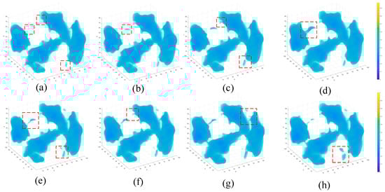
Figure 5. Eight consecutive stages. (a) Initial scattered damage clusters; (b) Upper damaged region becomes more concentrated; (c) Small upper branch appears; lower-right region slightly extends; (d) Upper damaged zone develops a more continuous shape; (e) Upper and lower damaged regions both expand; (f) Upper branch elongates along its growth direction; (g) Right-side damaged region enlarges noticeably; (h) Lower-right damaged zone thickens in the later stage. Red dashed squares mark the selected local areas for detailed observation.

3.2. Single-Step Prediction and Spatial Fidelity

A direct comparison between the true and predicted point clouds at one representative time step (Figure 6) demonstrates the high fidelity of the proposed STConvLSTM model. The overall structural similarity exceeds 90%, and the predicted accuracy reaches 92.6%, confirming that the model effectively reconstructs both the shape and extension trend of the actual damage zone.

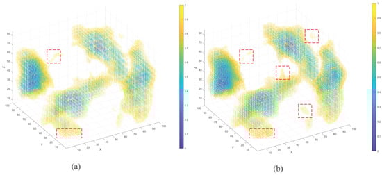
Figure 6. Comparison diagram: (a) real point cloud, (b) predicted point cloud. Red dashed squares mark the selected local areas for detailed observation.

Discrepancies, highlighted by red boxes in Figure 6, mainly occur near multi-damage intersections or along the damage boundaries—regions of high stress concentration and nonlinear deformation. This observation aligns with the known degradation of predictive accuracy in multi-damage interference zones, where local stress superposition and fracture bifurcation produce complex evolution paths.

3.3. Error Distribution Analysis

To further quantify prediction reliability, the spatial distribution of errors between the predicted and real data was analyzed (Figure 7). Most regions, especially the damage core, display low residuals close to zero, reflecting high overall accuracy and consistency with experimental data. The predicted results achieve an accuracy of 0.926, F1 = 0.947, and point cloud coverage = 0.975, indicating that nearly the entire damaged volume is captured. The structural similarity index (SSIM = 0.884) also supports excellent agreement in spatial topology.

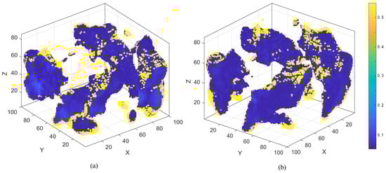
Figure 7. Relative error distribution: (a) front view, (b) perspective view after rotation by 180 degrees.

Higher errors at boundary areas result from temporal uncertainty propagation in multi-path evolution: although fine voxelization alleviates this issue, the temporal model tends to output conservative, probabilistic boundary predictions, leading to a slight overestimation of the damage extent.

A more detailed inspection of the error patterns in Figure 6 and Figure 7 reveals that the regions of higher deviation—primarily located at multi-damage intersections and along complex boundary morphologies—are closely linked to two intrinsic limitations of the current framework. First, although the physics-constrained loss effectively promotes continuity and smoothness, its soft-regularization nature cannot fully capture the abrupt changes in stress gradients or crack bifurcation events occurring in highly unstable boundary regions. This limitation partly explains the localized overestimation at branching or merging zones. Second, despite the use of density-adaptive voxelization, extremely intricate damage geometries may still exceed the effective spatial resolution achievable by the voxel grid. Fine-scale curvature and high-frequency morphological variations can thus be partially smoothed, leading to boundary blurring and slight spatial offsets between the predicted and true damage fronts. These findings highlight that the major sources of error lie not in the temporal modeling but in the difficulty of representing highly complex spatial–mechanical interactions, particularly under strong heterogeneity. Future improvements may incorporate curvature-aware constraints or multi-scale residual voxel refinement to mitigate these effects.

3.4. Cross-Sectional Validation

To visualize local prediction quality, cross-sections of error distribution at specific coordinates (X = 1, 21; Y = 1, 21; Z = 21, 41) were analyzed within the 100 × 100 × 100 voxel space (Figure 8). Most regions exhibit blue–green low-error zones, consistent with the high global similarity reported above. Red–yellow patches, representing larger deviations, appear mainly near complex geometric boundaries, implying potential improvement space for future boundary-refinement modules.

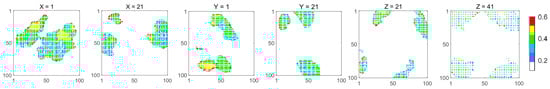
Figure 8. Error distribution cross-sectional chart.

3.5. Temporal-Step Prediction Verification

The model was also tested for multi-step temporal reasoning: using two historical time frames (t − 1, t) to predict the next one (t + 1). As shown in Figure 9, the predicted expansion trend matches the pattern observed in prior steps, with a spatial structure similarity exceeding 90%. Even without direct ground-truth comparison at this step, the consistency of propagation confirms that the model has learned stable spatiotemporal dynamics rather than memorizing static frames.

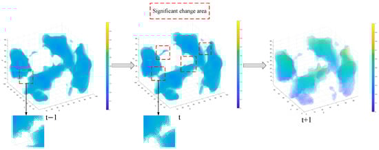
Figure 9. Verification, the two time steps ahead predict the next time step.

3.6. Comparative Study with Baseline Models

To evaluate overall performance, STConvLSTM was compared against 3D CNN [29], ConvLSTM [30], and UNet3D [31] baselines (Table 2). STConvLSTM achieved the highest accuracy (0.926) and F1-score (0.947), while maintaining competitive recall and coverage (0.975 each). ConvLSTM slightly exceeded STConvLSTM in recall due to its tendency to over-predict damaged zones, but this comes at the cost of precision. These results demonstrate that the proposed physics-constrained model effectively balances recall and precision, improving both numerical accuracy and physical consistency of the predicted evolution (Table 2). It is also noted that the numerical similarity between recall and PC-Coverage arises naturally from the voxel-wise prediction formulation, where both metrics measure the proportion of correctly identified damaged points (TP/(TP + FN)). PC-Coverage is nevertheless reported independently, because it emphasizes the spatial completeness of the reconstructed damage point cloud.

Table 2. Single-step prediction performance of different models on the test set (mean ± std over three independent runs).

Model Name	MSE	MAE	Accuracy	Recall	F1 Score	PC-Coverage
3D CNN	0.0181 ± 0.0017	0.0604 ± 0.0051	0.9122 ± 0.0041	0.9541 ± 0.0053	0.9332 ± 0.0043	0.9541 ± 0.0053
ConvLSTM	0.0152 ± 0.0013	0.0503 ± 0.0042	0.9030 ± 0.0049	0.9781 ± 0.0038	0.9391 ± 0.0037	0.9781 ± 0.0038
UNet3D	0.0301 ± 0.0022	0.1103 ± 0.0074	0.8420 ± 0.0062	0.8941 ± 0.0071	0.8670 ± 0.0064	0.8941 ± 0.0071
STConvLSTM	0.0121 ± 0.0011	0.0451 ± 0.0033	0.9261 ± 0.0034	0.9751 ± 0.0042	0.9470 ± 0.0035	0.9751 ± 0.0042

To further validate that the performance improvements of the proposed STConvLSTM model are not due to random variation, a statistical significance analysis was conducted on the metrics reported in Table 2. Each model was independently trained and evaluated over three randomized trials, and the resulting accuracy and F1-score values were subjected to a paired two-tailed Student’s t-test. The STConvLSTM achieved significantly higher accuracy and F1-score than the baseline models (3D CNN, ConvLSTM, and UNet3D), with p-values < 0.01 in all paired comparisons. These low p-values confirm that the observed performance gains are statistically significant rather than being attributable to random fluctuations in training. The inclusion of mean ± standard deviation in Table 2 further demonstrates the stability and reproducibility of the proposed method across repeated experiments.

3.7. Ablation Experiments

Ablation tests (Table 3) were designed to quantify the contributions of key modules:

Table 3. Ablation study results evaluating the contribution of adaptive voxelization and the composite loss function.

Model Configuration	Accuracy	Recall	F1 Score	PC-Coverage
STConvLSTM (Fixed Voxel + Composite Loss)	0.868	0.991	0.925	0.991
STConvLSTM (Adaptive Voxel + MSE Only)	0.853	0.996	0.906	0.966
STConvLSTM (Complete Model)	0.924	0.970	0.947	0.970

• Removing adaptive voxelization (fixed voxels + composite loss);
• Replacing the composite loss with simple MSE (adaptive voxels + MSE only);
• The complete model.

The complete model achieves the highest accuracy and F1-score. Compared with the MSE-only model, accuracy improves by 8.3% and F1-score by 4.5%; compared with the fixed-voxel model, accuracy improves by 6.5% and F1-score by 2.4%. While the simplified models achieve higher recall and coverage, this is a result of their tendency to over-predict the damaged area, which artificially inflates these metrics at the cost of precision. Such over-prediction reduces practical reliability, as excessive false positives can trigger unnecessary alerts or misallocate computational resources in real applications. Removing the composite loss leads to noticeably reduced physical consistency and accuracy, confirming that this module is essential for preserving physically plausible damage evolution. Removing adaptive voxelization causes detail loss and increases redundant computation in sparse regions. Together, the two modules act synergistically to produce the best overall performance.

The experimental findings show that boundary errors also arise from temporal uncertainty: when the predicted damage initiates slightly earlier or later than the ground truth, these subtle timing deviations propagate into visible spatial shifts along complex fracture fronts. Although such residual misalignments persist near intricate boundaries, the method remains robust and yields consistent performance in forecasting overall damage evolution. Future work will focus on refining boundary modeling and enhancing multi-physics coupling to further strengthen predictive reliability.

4. Discussion

In the context of performance, our model compares favorably against 3D CNN, ConvLSTM, and UNet3D baselines, achieving the highest accuracy (0.926) and F1-score (0.947) while maintaining competitive recall and point cloud coverage (0.975). ConvLSTM’s slight recall advantage stems from over-prediction, traded off against precision. These observations support that physics-aware regularization improves precision without sacrificing detectability. They are reinforced by our ablation tests showing that removing the composite loss or adaptive voxelization degrades accuracy/F1 or detail retention, respectively, confirming the necessity of both modules.

Regarding data representation, damage point clouds are sparse, and heterogeneous, fixed-resolution voxelization loses critical details. Our density-adaptive point cloud↔voxel conversion preserves fine structures in dense regions while keeping computation tractable, forming an effective interface to volumetric learners. This design choice is consistent with evidence that point–voxel fusion and sparse 3D convolutions (PVCNN, Submanifold Sparse Conv, Minkowski) enhance efficiency and fidelity in sparse 3D fields [14,15,16]. Together with a 3D encoder–decoder pathway—a proven volumetric baseline typified by 3D U-Net—it provides the spatial context that standard ConvLSTM lacks [21].

From the perspective of physical regularization, purely data-driven models can drift from mechanics, yielding torn or over-diffuse fronts [17,18]. Our composite loss introduces continuity and smoothness terms (Griffith-motivated) and an edge-distribution constraint related to the stress-intensity factor $K_I$, plus a one-sided over-prediction penalty. Collectively these steer predictions toward mechanically admissible morphologies and curb non-physical expansion. This approach aligns with theory-guided learning and recent phase-field/PINN fracture studies that embed energy consistency to improve plausibility [19].

In examining the error distribution, residuals cluster at multi-damage interference zones and along complex boundaries—regions of high stress concentration and multi-path evolution—precisely where temporal uncertainty propagates and models tend to output conservative, probabilistic fronts. Cross-sectional views confirm low error in cores but larger deviations near intricate geometries, indicating room for boundary-refinement modules.

From a practical application standpoint, given the strong accuracy/F1 and physically consistent morphologies, the method is well suited to early-warning and support-design scenarios in underground engineering, provided domain calibration is performed. This aligns with emerging multi-sensor early-warning frameworks (MS–AE–EMR), where deep learning improves risk assessment timeliness [32], and with the broader thrust of theory-guided data science in geomechanics [18].

Despite these promising results, several limitations point to clear directions for future improvement, including (1) boundary refinement via curvature-aware or energy-aware regularization (e.g., boundary/phase-field surrogates) to reduce local errors; (2) stronger volumetric saliency using boundary-focused attention; (3) multi-physics coupling (e.g., fusing AE with ultrasonic velocity/IR fields) to better constrain edge behavior under high stress gradients; (4) broader validation across lithologies, loading paths, and field heterogeneity for deployment readiness [19,32,33]. Our experiments and error maps suggest these steps are the most impactful next moves.

5. Conclusions

This study presents a physics-constrained spatiotemporal framework that effectively addresses the challenges of data heterogeneity and physical inconsistency commonly encountered in rock-damage prediction. By combining density-adaptive point cloud-to-voxel conversion with a composite loss function rooted in fracture mechanics, the proposed method achieves accurate and physically interpretable spatiotemporal forecasting of damage evolution under uniaxial compression.

The model attains a prediction accuracy of 92.6% and an F1-score of 0.947 on acoustic emission datasets, substantially outperforming conventional 3D CNN, ConvLSTM, and UNet3D baselines. Although the adaptive voxelization and physics-informed optimization introduce moderate additional computational overhead during training compared with purely data-driven counterparts, inference remains efficient and suitable for real-time monitoring. In safety-critical rock engineering applications such as mining and tunneling, the marked improvement in prediction precision and adherence to physical principles clearly justifies this modest increase in training cost.

Despite these advances, certain limitations persist, as discussed in Section 3.3 and Section 3.7, prediction errors are predominantly confined to regions featuring complex boundary morphologies, multi-damage intersections, and crack bifurcations. These arise from the challenge of capturing abrupt stress gradients and high-curvature features even with density-adaptive voxelization, as extremely intricate geometries can still push the limits of effective spatial resolution in the voxel representation, while minor temporal offsets further amplify spatial misalignment along delicate fracture fronts. Future work will address these issues by introducing curvature-aware constraints and multi-scale residual refinement, enhancing multi-physics coupling to improve temporal alignment, and validating the approach on in situ microseismic and full-scale field datasets to achieve higher boundary fidelity and broader practical applicability.

References

- Jiang, L.; Xiong, H.; Zeng, T.; Wang, J.; Xiao, S.; Yang, L. In-situ micro-CT damage analysis of carbon and carbon/glass hybrid laminates under tensile loading by image reconstruction and DVC technology. Compos. Part A Appl. Sci. Manuf. 2024, 176, 107844. [Google Scholar] [CrossRef]
- Tian, Y.; Li, H.; Wang, Y.; Ye, Q.; Guo, A. Gravity Gradient Inversion of Gravity Field and Steady-State Ocean Circulation Explorer Satellite Data for the Lithospheric Density Structure in the Qinghai–Tibet Plateau Region and the Surrounding Regions. J. Geophys. Res. Solid Earth 2021, 126, e2020JB021291. [Google Scholar] [CrossRef]
- Zhou, W.; Qin, R.; Han, K.N.; Wei, Z.Y.; Ma, L.H. Progressive damage visualization and tensile failure analysis of three-dimensional braided composites by acoustic emission and micro-CT. Polym. Test. 2021, 93, 106881. [Google Scholar] [CrossRef]
- Yang, Z.; Cheng, Z.; Wu, D. Deep learning driven prediction and comparative study of surrounding rock deformation in high speed railway tunnels. Sci. Rep. 2025, 15, 24104. [Google Scholar] [CrossRef]
- Shi, L.L.; Zhang, J.; Zhu, Q.Z.; Sun, H.H. Long-term and short-term constitutive model of rock based on deep learning and deformation prediction of sandy limestone. Rock Soil Mech. 2025, 46, 289–302. [Google Scholar] [CrossRef]
- Liu, R.; Wang, Z.; Zhang, Y.; Yao, X.; Yan, S.; Chen, Z.; Wang, S.; Li, H.; Wang, Q. Research on rock fracture evolution prediction model based on Adam-ConvLSTM and transfer learning. Discov. Appl. Sci. 2025, 7, 217. [Google Scholar] [CrossRef]
- Zhang, D.; Zhang, Y.; Jiao, S.; Zhao, Y.; Deng, W.; Xue, B.; Wen, X. Prediction Method for Surface Settlement during Underground Mining in Mines Based on LSTM-DCNN and Transfer Learning. Min. Res. Dev. 2025, 1–9. [Google Scholar] [CrossRef]
- Li, J.; Wang, Y.; Zhang, T.; Zhou, Y.; Luo, H.; Liu, X. Rockburst Intensity Prediction Model Based on Newton–Raphson Algorithm and BP Neural Network. Min. Res. Dev. 2025, 45, 127–133. [Google Scholar] [CrossRef]
- Zheng, L.; Liang, P.; Li, G.; Liu, Y.; Liu, T.; Wang, J. CNN-LSTM Rockburst Intensity Grade Prediction Model Based on Fusion Optimization Algorithm under Unbalanced Data. Min. Res. Dev. 2025, 45, 111–118. [Google Scholar] [CrossRef]
- Zhou, Y.; Tuzel, O. VoxelNet: End-to-End Learning for Point Cloud-Based 3D Object Detection. In Proceedings of the IEEE Conference on Computer Vision and Pattern Recognition (CVPR), Salt Lake City, UT, USA, 18–22 June 2018; pp. 4490–4499. [Google Scholar] [CrossRef]
- Qi, C.R.; Yi, L.; Su, H.; Guibas, L.J. PointNet++: Deep hierarchical feature learning on point sets in a metric space. In Proceedings of the Advances in Neural Information Processing Systems (NeurIPS), Long Beach, CA, USA, 4–9 December 2017; pp. 5099–5108. [Google Scholar] [CrossRef]
- Zhao, H.; Xiao, Z. PVLF: Point–Voxel Local Feature Fusion for 3D Detection. Discov. Artif. Intell. 2025, 5, 93. [Google Scholar] [CrossRef]
- Guo, Y.; Wang, H.; Hu, Q.; Liu, H.; Liu, L.; Bennamoun, M. Deep Learning for 3D Point Clouds: A Survey. IEEE Trans. Pattern Anal. Mach. Intell. 2021, 43, 4338–4364. [Google Scholar] [CrossRef]
- Liu, Z.; Tang, H.; Lin, Y.; Han, S. Point–Voxel CNN for Efficient 3D Deep Learning. In Proceedings of the Advances in Neural Information Processing Systems (NeurIPS), Vancouver, BC, Canada, 8–14 December 2019. [Google Scholar] [CrossRef]
- Graham, B.; van der Maaten, L. Submanifold Sparse Convolutional Networks. In Proceedings of the IEEE Conference on Computer Vision and Pattern Recognition (CVPR), Salt Lake City, UT, USA, 18–22 June 2018. [Google Scholar] [CrossRef]
- Choy, C.; Gwak, J.; Savarese, S. 4D Spatio-Temporal ConvNets: Minkowski Convolutional Neural Networks. In Proceedings of the IEEE Conference on Computer Vision and Pattern Recognition (CVPR), Long Beach, CA, USA, 15–20 June 2019. [Google Scholar] [CrossRef]
- Raissi, M.; Perdikaris, P.; Karniadakis, G.E. Physics-informed neural networks. J. Comput. Phys. 2019, 378, 686–707. [Google Scholar] [CrossRef]
- Karpatne, A.; Atluri, G.; Faghmous, J.H.; Steinbach, M.; Banerjee, A.; Ganguly, A.; Shekhar, S.; Samatova, N.; Kumar, V. Theory-Guided Data Science: A New Paradigm for Scientific Discovery from Data. IEEE Trans. Knowl. Data Eng. 2022, 34, 3924–3938. [Google Scholar] [CrossRef]
- Manav, M.; Molinaro, R.; Mishra, S.; De Lorenzis, L. Phase-field modeling of fracture with physics-informed deep learning. Comput. Methods Appl. Mech. Eng. 2024, 429, 117104. [Google Scholar] [CrossRef]
- Karniadakis, G.E.; Kevrekidis, I.G.; Lu, L.; Perdikaris, P.; Wang, S.; Yang, L. Physics-informed machine learning. Nat. Rev. Phys. 2021, 3, 422–440. [Google Scholar] [CrossRef]
- Çiçek, Ö.; Abdulkadir, A.; Lienkamp, S.S.; Brox, T.; Ronneberger, O. 3D U-Net: Learning dense volumetric segmentation from sparse annotationn. In Medical Image Computing and Computer-Assisted Intervention—MICCAI 2016, Proceedings of the 19th International Conference, Athens, Greece, 17–21 October 2016; Lecture Notes in Computer Science; Springer: Berlin/Heidelberg, Germany, 2016; Volume 9901, pp. 424–432. [Google Scholar] [CrossRef]
- Zhang, L.; Lu, L.; Wang, X.; Zhu, R.M.; Bagheri, M.; Summers, R.M.; Yao, J. Spatio-Temporal ConvLSTMs for Tumor Growth Prediction by Learning 4D Longitudinal Patient Data. arXiv 2019, arXiv:1902.08716. [Google Scholar] [CrossRef]
- Yao, X.; Zhang, Y.; Sun, L.; Yang, Z.; Liu, X.; Liang, P. Research on Rock Damage Acoustic Emission Detection and Imaging Method Based on Regional Correlation. Chin. J. Rock Mech. Eng. 2017, 36, 2113–2123. [Google Scholar] [CrossRef]
- Yao, X.; Liu, Z.; Zhang, Y.; Tao, Z.; Liang, P.; Zhao, J. Effect of regionalized structures on rock fracture process. Sci. Rep. 2024, 14, 10490. [Google Scholar] [CrossRef]
- Cheng, Y.; Hagan, P.; Mitra, R.; Wang, S.; Yang, H.-W. Experimental investigation of progressive failure using 3D acoustic emission tomography. Front. Earth Sci. 2021, 9, 765030. [Google Scholar] [CrossRef]
- Song, T.; Zhou, Y.; Yu, X. Three-Dimensional AE Source Localization for Layered Rock Considering Anisotropic P-Wave Velocity. Bull. Eng. Geol. Environ. 2024, 83, 185. [Google Scholar] [CrossRef]
- Woo, S.; Park, J.; Lee, J.-Y.; Kweon, I.S. CBAM: Convolutional Block Attention Module. In Proceedings of the European Conference on Computer Vision (ECCV), Munich, Germany, 8–14 September 2018. [Google Scholar] [CrossRef]
- Wang, J.; Yu, Z.; Luan, Z.; Ren, J.; Zhao, Y.; Yu, G. RDAU-Net: Residual CNN with DFP and CBAM for Brain Tumor Segmentation. Front. Oncol. 2022, 12, 805263. [Google Scholar] [CrossRef]
- Ji, S.; Xu, W.; Yang, M.; Yu, K. 3D convolutional neural networks for human action recognition. IEEE Trans. Pattern Anal. Mach. Intell. 2013, 35, 221–231. [Google Scholar] [CrossRef]
- Shi, X.; Chen, Z.; Wang, H.; Yeung, D.-Y.; Wong, W.-K.; Woo, W.-C. Convolutional LSTM network: A machine learning approach for precipitation nowcasting. In Proceedings of the Advances in Neural Information Processing Systems 28 (NeurIPS 2015, Montreal, QC, Canada, 7–12 December 2015; pp. 802–810. [Google Scholar]
- Yu, X.; Wu, Y.; Bai, Y.; Han, H.; Chen, L.; Gao, H.; Wei, H.; Wang, M. A lightweight 3D UNet model for glioma grading. Phys. Med. Biol. 2022, 67, 155006. [Google Scholar] [CrossRef]
- Di, Y.; Wang, E.; Li, Z.; Liu, X.; Huang, T.; Yao, J. Comprehensive early warning of rockburst from MS–AE–EMR signals via deep learning. Int. J. Rock Mech. Min. Sci. 2023, 170, 105519. [Google Scholar] [CrossRef]
- Kervadec, H.; Bouchtiba, J.; Desrosiers, C.; Granger, E.; Dolz, J.; Ben Ayed, I. Boundary loss for highly unbalanced segmentation. Med. Image Anal. 2021, 67, 101851. [Google Scholar] [CrossRef] [PubMed]
Disclaimer/Publisher’s Note: The statements, opinions and data contained in all publications are solely those of the individual author(s) and contributor(s) and not of MDPI and/or the editor(s). MDPI and/or the editor(s) disclaim responsibility for any injury to people or property resulting from any ideas, methods, instructions or products referred to in the content. |
© 2025 by the authors. Licensee MDPI, Basel, Switzerland. This article is an open access article distributed under the terms and conditions of the Creative Commons Attribution (CC BY) license (https://creativecommons.org/licenses/by/4.0/).