Artificial Intelligence-Driven Project Portfolio Optimization Under Deep Uncertainty Using Adaptive Reinforcement Learning

Abstract

This study proposes an adaptive reinforcement learning (ARL) framework for optimizing project portfolios under deep uncertainty. Unlike traditional static approaches, our method treats portfolio management as a dynamic learning problem. It integrates both explicit and tacit knowledge flows. The framework employs ensemble Q-learning with meta-learning capabilities and adaptive exploration–exploitation mechanisms. We validated our approach across 84 organizations in five industries. The results show significant improvements: 68% in resource allocation efficiency and 52% in strategic alignment (both p < 0.01). The ARL algorithm continuously adapts to emerging patterns while maintaining strategic coherence. Key contributions include (1) reconceptualizing portfolio optimization as learning rather than allocation, (2) integrating tacit knowledge through fuzzy linguistic variables, and (3) providing calibrated implementation protocols for diverse organizational contexts. This approach addresses fundamental limitations of existing methods in handling deep uncertainty, non-stationarity, and knowledge integration challenges.

1. Introduction

Project portfolio management (PPM) is a strategic function for organizations operating in complex business environments. The selection, prioritization, and management of projects in a portfolio ensure that the organization’s ability to meet strategic objectives while optimizing resource use [1,2]. According to Gholizadeh et al. [3], organizations face tremendous uncertainty from economic instability, technological disruption, geographical factors, and changing stakeholder expectations. Therefore, sophisticated approaches are needed for PPM decision-making.

Classical portfolio optimization models are mainly based on deterministic methods or oversimplified probabilistic ones that do not address the multifaceted uncertainties in the project context properly [4,5]. The assumptions made by traditional methods, such as stable circumstances with fixed parameters and probability distributions, hardly represent the reality and complexity of modern project portfolios [6,7]. As project environments keep becoming more complex, there is a need for more flexible and robust methodologies that could work in a “deep uncertainty”, which means that the decision-maker does not completely know (i) the value of system parameters, (ii) the probability distribution of any of these parameters, or (iii) the possible future states of even the full set of models [8,9]. Artificial intelligence (AI) and machine learning (ML) techniques have come up as promising solutions to these challenges. Their capabilities to recognize patterns, learn from data, and adapt to dynamic conditions [10,11] can be quite useful in the context of missing data.

Reinforcement learning (RL) may provide some particularly useful functionalities for portfolio optimization under uncertainty. RL is the machine learning branch where agents learn optimal behavior by interacting with the environment [12,13]. Reinforcement learning (RL) is distinctly different from supervised learning approaches that require labeled data. RL enables the optimization of decision policies by balancing exploration (discovering the unknown) and exploitation (using the known). This is well-captured in the pace of the dynamism of project portfolio management [14,15].

An overview of the literature reveals several research streams related to project portfolio optimization under uncertainty with various methodological approaches and optimization techniques.

Various researchers have studied multi-objective optimization frameworks of project portfolio selection and emphasized the necessity of balancing conflicting objectives. Khalili-Damghani et al. [16] proposed a hybrid, fuzzy, multiple-criteria decision-making with a sustainability dimension. By a similar token, Abbasi and others [17] utilized a balanced scorecard model for new product development portfolio selection based on financial and non-financial criteria. Researchers RezaHoseini et al. [18] developed a comprehensive mathematical model in which resource constraints and sustainability factors were considered in project selection and scheduling. In another approach, Khalilzadeh and Salehi [19] considered social responsibility and risk in a multi-objective fuzzy model.

There is a growing trend towards integrating dimensions of sustainability into portfolio optimization models. For example, Kudratova et al. [20] investigated sustainable project selection under reinvestment strategies, and Gholizadeh et al. [21] coupled uncertainty with sustainable–green integrated logistics networks. This reveals that more projects are selected because of their environmental and social merits; not just economic ones.

Numerous investigations have been conducted into robust optimization techniques to deal with uncertainty in project portfolio selection. Mahmoudi et al. [1] offered a novel framework by using a strong ordinal priority approach for improving organizational resilience. Hassanzadeh and colleagues [6] designed a strong R&D project portfolio model for pharmaceutical firms, considering market and technical uncertainties. In the same way, Gholizadeh et al. [3] presented an extensive fuzzy stochastic programming methodology for sustainable procurement under hybrid uncertainty.

The incorporation of biodata analytics within a robust optimization framework is an emerging trend. Govindan et al. [22] utilize big data to develop resilience in network design. Most of these approaches focus on good solutions for all or many possible futures rather than making the best of one expected future.

Because project portfolios are not static, much research has been conducted to enable adaptation to changing conditions. Shen et al. [2] proposed a new extended model of a dynamic project portfolio selection based on project synergy and interdependency factors. Tavana et al. [5] worked on a dynamic two-stage programming model for project evaluation and selection under uncertainty. Also, Jafarzadeh et al. [23] investigated optimal portfolio selection with reinvestment flexibility over a changing time horizon.

Portfolio optimization possesses a temporal dimension, which has been explored by Ranjbar et al. [24] and Tofighian and Naderi [25]. They propose integrated project selection and scheduling frameworks, which have an impact on the performance of the portfolio. As per these approaches, selection of a portfolio need not be a one-time decision, but we need to adjust the portfolio continuously.

We have been using artificial intelligence and machine learning for portfolio optimization problems. Conlon et al. [10] and Aithal et al. [26] used machine learning heuristics for real-time portfolio optimization. The above statement has a lot to say. Nafia et al. [14] used LSTM networks for stock prediction and portfolio construction, showing the promise of deep learning in finance.

Hybrid methods that combine classical optimization with AI techniques continue to have some promise. For example, Yeo et al. [15] propose a genetic algorithm approach that utilizes a neural network for dynamic portfolio rebalancing, while Zhang et al. [27] propose a hybrid portfolio selection procedure that factors in historical performance. All authors in the literature reviewed above employ advanced hybrid models to combine stock selection or enhanced portfolio rebalancing with genetic algorithms and other methods like neural networks and support vector regression.

Different researchers have researched the complex interdependencies of a project in a portfolio. As per Alvarez-García and Fernández-Castro [28], a complete approach was presented for choosing interdependent projects. Pajares and López [29] also researched methodological approaches for taking interactions in a project and a portfolio into account. Wu et al. [9] studied project interaction under different enterprise strategic scenarios since interaction between projects can enhance the performance of the portfolio.

The papers of Shariatmadari et al. [30], who used integrated resource management frameworks, and Jahani et al. [31], who studied multi-stage manufacturing within supply chain design, further explore the systemic nature of project portfolios. The approaches above make it necessary not to consider a particular project as an isolated activity, but rather as a subset of a larger project.

Although there are important developments in project portfolio optimization methodologies, a thorough analysis of the literature shows clear epistemological and methodological gaps. Studies conducted by Gholizadeh et al. [3], Mahmoudi et al. [1], Perez et al. [32], and Bairamzadeh et al. [8] indicate that optimization models that are currently in use work efficiently to handle uncertainties that are already known. However, they do not learn from uncertainties that become known throughout projects. Deterministic, or simplified probabilistic, approaches tend to generate static solutions. Thus, as conditions evolve, they lose their optimality. This problem is quite visible in Tavana et al. [5], Liu et al. [4], and Wu et al. [9].

A study of the literature reveals that the insufficient accounting of deep uncertainty is a core problem of existing paradigms. Hassanzadeh et al. [6] and Huang and Zhao [7] pointed out that existing approaches mostly deal with stochastic uncertainty (with known probability distributions) or interval uncertainty (with parameters varying within known bounds). They are poorly equipped to deal with deep uncertainty when the probabilities are unknown or even, when possible, states are unknown. The portfolio optimization processes have not been properly integrated into explicit and tacit knowledge, which has been articulated more recently by Khalili-Damghani et al. [33] and Lukovac et al. [34].

Another systematic issue that Hu et al. [12] and Rather [13] discover is the rigid exploration–exploitation balance. Today’s models often use fixed strategies to balance exploration (which is discovering new things) versus exploitation (which is using already-known information). But they often do not have ways that can change this balance.

The research of Yeo et al. [15] and Zhang et al. [27] has documented another major gap, which is inadequate consideration of the non-stationary characteristics of project environments, which reveal changing underlying system dynamics and parametric relationships over time. When this issue is combined with problems raised by RezaHoseini et al. [18], Abbasi et al. [17], and Kudratova et al. [20], it can be inferred that more flexible optimization frameworks are urgently required, from which such multiple uncertainties can easily be dealt with.

Based on a systematic review of the literature, including the larger works of Conlon et al. [10], Kaucic [35], and Gunjan and Bhattacharyya [11], as well as the more focused work of Shen et al. [2], Alvarez-García and Fernández-Castro [28], and Khalilzadeh and Salehi [19], it is clear something is missing from the current paradigms. In spite of the efforts of Tavana et al. [36], Jafarzadeh et al. [23], and Nafia et al. [14], there is a lack of an integrated approach for simultaneously addressing learning limitations, representing deep uncertainty, integrating explicit and tacit knowledge, dynamically balancing exploration and exploitation, and recognizing the non-stationary nature of projects. The critical studies of Chou et al. [37], Bocewicz et al. [38], Ranjbar et al. [24], and Jahani et al. [31] highlight the research gaps, which require a shift in paradigm. In other words, project portfolio optimization must not be conceived of as a resource allocation problem, but rather as a non-stationary learning problem [39].

Recent research has made further progress in portfolio optimization theory and methodology under uncertainty. Miri et al. [40] proposes robust portfolio selection frameworks using deep learning architectures to address model ambiguity. Their paper illustrates that distributional uncertainty can be systematically managed through a neural network-based approach. By managing model ambiguity through ensemble deep learning techniques in a structured manner, these authors provide an interesting insight for uncertainty quantification, primarily directed towards financial assets’ allocation and not for knowledge-rich project portfolio optimization. The authors (Muteba Mwamba et al.) [41] of this paper proposed multi-objective portfolio optimization through the Non-Dominated Sorting Genetic Algorithm III. It could be better to explore the Pareto frontier of conflicting objectives. Although the methodology is applied to multi-criteria decision-making for portfolios, it uses static optimization paradigms that do not employ dynamic learning mechanisms, which are crucial in non-stationary settings.

In a study recently conducted by Shan et al. [42], dynamic adaptation pathways were developed for infrastructural systems facing uncertain climate scenarios within the larger challenge of decision-making under deep uncertainty Their framework for managing deep uncertainty—defined as situations where no probability distributions are known, and which rely on incomplete knowledge of system dynamics—can provide methodological insights that are not limited to a specific application. Their stress on adaptable pathways subject to profound uncertainty lends critical weight to the necessity of learning-based approaches—the use of adaptation when optimization fails in the face of essential uncertainty regarding system behavior and the environment.

To tackle these deficiencies, this study formulates an adaptive reinforcement learning framework geared toward project portfolio optimization under deep uncertainty. The proposed approach will view portfolio optimization as a non-stationary learning problem instead of a resource allocation problem with a single point-in-time goal. Its objectives are as follows:

• To develop a mathematical model incorporating dynamic state representations that capture both explicit and tacit knowledge flows across interconnected projects.
• To design an adaptive reinforcement learning algorithm that continuously optimizes the exploration–exploitation balance based on emergent patterns in the portfolio environment.
• To empirically validate the proposed framework through longitudinal testing across multiple organizations and industries, demonstrating improvements in resource allocation efficiency and strategic alignment.

We improve existing methods in several important ways. To begin with, we consider a state representation that combines quantitative parameters with qualitative knowledge ones. This allows for a better understanding of the state of the portfolio environment. In addition, we create a reinforcement learning algorithm that can detect and adapt to fundamental changes in the system dynamics rather than just the parameters. We introduce a meta-learning mechanism to our algorithm, enabling it to learn faster as it transfers knowledge across portfolios.

Empirical validation of our technique in 84 organizations in five industries results in a 68% improvement in resource allocation efficiency and a 52% enhancement in strategic alignment as against traditional portfolio management techniques. Describing portfolio optimization as learning rather than optimization helps organizations in deep uncertainty environments. This study contributes towards both theory and practice in several ways.

• This study reconceptualizes project portfolio optimization as a non-stationary learning problem. It challenges the dominant paradigm of static resource allocation. The idea shift can have interesting theoretical implications for thinking about how organizations learn and change in messy environments.
• We designed a new reinforcement learning framework for project portfolio settings, which systematically controls the exploration–exploitation trade-off, integrates explicit and tacit knowledge, and incorporates changing dynamics of the system.
• With extensive testing in several organizations and industries, adaptive learning has been shown here to significantly improve resource allocation efficiency and strategic alignment regarding portfolio optimization.
• For practitioners, we offer a calibrated implementation framework that is flexible and can be used in various organizational contexts, as well as guidance on making the approach consistent with existing portfolio management processes.

The rest of the paper is arranged as follows: In Section 2, we elaborate on the theory and math behind our adaptive reinforcement learning framework. In Section 3, research methodology is discussed (data collection, experiments, and validation). Section 4 discusses actual findings from longitudinal testing performed in several organizations and industries. Section 5 explores how our findings can affect theory and practice. It also highlights the limitations and future research directions. In the end, Section 6 summarizes key contributions and their significance for project portfolio optimization under deep uncertainty.

2. Theoretical Foundation and Mathematical Formulation

This section provides the theoretical foundations and mathematical formulation of the adaptive reinforcement learning (ARL) framework, which we developed to optimize project portfolios under deep uncertainty. Referencing the shortcomings highlighted in the existing literature, we reimagine portfolio optimization as a non-stationary learning problem instead of a stationary allocation problem. This transformation allows the project ecosystem to continuously adapt to emerging patterns while also using explicit and tacit knowledge flows.

The suggested framework aims to address the five shortcomings of existing approaches, which are (1) limited learning, (2) shallow representation of deep uncertainty, (3) an unduly rigid exploration–exploitation balance, (4) insufficient operability of explicit and tacit knowledge, and (5) lack of attention to non-stationarity. We start by formalizing the problem of project portfolio optimization under deep uncertainty, then introducing the ARL model and its specifications.

2.1. Problem Formulation

We define the project portfolio optimization process as a dynamic decision-making process under deep uncertainty. Consider an organization that has several projects represented as P = p₁, p₂, …, p_n. Each project pi has attributes A = ai₁, ai₂, …, ai_m.

The attributes include expected returns, resource requirements, alignment with strategy, the risk profile, and synergy with other projects.

In the face of pervasive uncertainty, the actual values of these may initially be imprecise, and their values could evolve due to changing market conditions, technological advances, organizational priorities, and other exogenous factors. Furthermore, no exhaustive understanding of how projects relate to each other or the degree to which external factors impact performance exist. We need a flexible and adaptable approach that we learn when new information comes to light.

The portfolio optimization problem can be formally stated as follows. Determine a subset of P, P* ⊆ P and resource allocation R* = {r₁, r₂, …, rₙ}, which maximizes the expected value of portfolio V(P*, R*) subject to resource constraints and strategic considerations:

$$\underset{P^{*}\subseteq P,R^{*}}{max}E\left[V\left(P^{*},R^{*}\right)\right]P^{*}\subseteq P,R^{*}$$

(1)

$$\mathrm{subject} \mathrm{to} {\sum }_{p_i\in P^{*}}{r}_i\le R_{total}$$

(2)

$$r_i\ge 0,\forall p_i\in P^{*}$$

(3)

$$S\left(P^{*}\right)\ge S_{min}$$

(4)

In the equation, R_total is the total available resources, S(P*) is the strategic alignment of the portfolio, and S_min is the minimum acceptable level of strategic alignment. We consider an optimization problem from a deep uncertainty perspective. Unlike the traditional approach, which assumes a model structure, parameters, and values that are static and fully known, we take the position that the true model structure, true parameter values, and even possible future states are not fully known. To systematically address different uncertainty types in portfolio optimization, we establish a comprehensive taxonomy following Walker et al. [39] and Bairamzadeh et al. [8]. Table 1 characterizes three fundamental uncertainty categories with their corresponding mathematical treatments and practical examples from portfolio management contexts.

Table 1. Uncertainty taxonomy and mathematical treatment in portfolio optimization.

Uncertainty Type	Definition	Example in Portfolio Context	Mathematical Treatment
Aleatory	Natural variability, irreducible randomness	Market demand fluctuations, competitor actions	P(X) known, Monte Carlo simulation
Epistemic	Knowledge limitations, reducible through learning	Technology maturation rates, team capabilities	P(θ|D) Bayesian updating
Deep	Unknown model structures, incomplete state space	Disruptive innovations, regulatory paradigm shifts	Model ensemble M ∈ {M1, …, Mk}

2.2. Reinforcement Learning Framework

The portfolio optimization problem we consider will be formulated as a Markov Decision Process (MDP) with non-stationary dynamics defined by the notations ⟨S, A, P, R, γ⟩, where S is the state space, A is the action space, P is the probabilistic state transition, R is the reward function, and γ is the discount factor. A new adaptation mechanism is introduced to cope with non-stationarity and deep uncertainty.

2.2.1. State Space Representation

The current combination of portfolios, funding, organizational context, and knowledge state is represented by the state space S. An important feature in our approach is a state representation that utilizes explicit and tacit knowledge information. We define the state vector s_t at time t as

$$s_t=\left[P_t,R_t,E_t,T_t,C_t\right]$$

(5)

where

• $P_t=p^{1t},p^{2t},\dots ,{p_n}^t$ represents the binary indicators for project selection in the current portfolio $\left(p_i^t\in 0,1\right)$;
• $R_t=r^{1t},r^{2t},\dots ,{r_n}^t$ denotes the resource allocation across selected projects;
• $E_t=e^{1t},e^{2t},\dots ,{e_m}^t$ captures explicit knowledge dimensions (quantifiable metrics);
• $T_t=t^{1t},t^{2t},\dots ,{t_k}^t$ represents tacit knowledge dimensions (experiential insights);
• $C_t=c^{1t},c^{2t},\dots ,{c_l}^t$ describes the contextual factors (organizational, market, technological).

In the vector of explicit knowledge, E_t, we include observable aspects such as realized returns, allocative efficiency, schedule compliance, and quality. Following the work of Mahmoudi et al. [1] and Hassanzadeh et al. [6], we extend these quantifiable dimensions to uncertainty measures and sensitivity indicators. The tacit knowledge vector T_t, a unique feature of our model, captures experiential insights that are not directly quantifiable but significantly influence decision-making. In keeping with the work of Lukovac et al. [34], we operationalized tacit knowledge using fuzzy linguistic variables that emerged from experts’ judgments, pattern recognition from historical choices, and knowledge flow modeling of inter-project dependencies.

This helps to include the intuitive judgment in the formal decision-making process.

Contextual factors C_t refers to the surroundings of portfolio decisions—standards and priorities of the organization, market trends, technological trends, and the regulatory environment. This component takes the context-sensitive approach developed by Wu et al. [9] and extends it with adaptive mechanisms for identifying contextual shifts.

2.2.2. Action Space

Action space A includes portfolio reconfiguration decisions such as project selection/deselection and resource reallocations. We define an action a_t at time t as

$$a_t=\left[\Delta P_t,\Delta R_t\right]$$

(6)

where

• $\Delta P_t=\Delta p^{1t},\Delta p^{2t},\dots ,\Delta {p_n}^t$ represents changes in project selection $\left(\Delta p_i^t\in -1,0,1\right)$;
• $\Delta R_t=\Delta r^{1t},\Delta r^{2t},\dots ,\Delta {r_n}^t$ denotes adjustments in resource allocation.

To deal with the problem of high-dimensional action spaces identified by Rather [13], we use a hierarchy of actions that decides portfolio-level actions first and project-level actions next. This approach, which draws on the paradigm of hierarchical reinforcement learning, enables high-quality decisions to be made with little computational effort.

2.2.3. Transition Dynamics Under Deep Uncertainty

The transition function $P\left(s_{t+1}|s_t,a_t,m\right)$ describes the process of how the system advances from state s_t to s_t+1 after applying action a_t. The transition dynamics, which are unknown under deep uncertainty, may change over time. We use a Bayesian model that maintains a probability distribution over possible transition models rather than a single fixed model.

Let M represent the space of possible transition models. At time t, we have a belief distribution b_t(m) over m ∈ M. We use Bayes’ rule to update the belief after observing a transition (s_t, a_t, s_t+1).

$$b_{t+1}\left(m\right)={\displaystyle \frac{P\left(s_{t+1}|s_t,a_t,m\right)\cdot b_t\left(m\right)}{{\sum }_{m^{\prime }\in M}P\left(s_{t+1}|s_t,a_t,m^{\prime }\right)\cdot b_t\left(m^{\prime }\right)}}$$

(7)

This Bayesian modeling helps the algorithm adjust to the evolving dynamics, and as it experiences, it can reduce the uncertainty. To do this in a way that is computationally tractable, we use a parametric family of transition models f(· θ), with parameter vector θ [10].

$$P\left(s_{t+1}|s_t,a_t,\theta \right)=f\left(s_t,a_t,\theta ,{ϵ}_t\right)$$

(8)

where f is a differentiable function and ϵ_t indicates external random factors. The belief distribution is stored over the parameter space Θ instead of the entire model space M.

2.2.4. Non-Stationary Reward Function

The reward function R(s_t, a_t, s_t+1) assigns a value to the transition from s_t to s_t+1 after taking the action a_t. The designed reward function is multi-dimensional, which serves to balance short- and long-term returns:

$$R\left(s_t,a_t,s_{t+1}\right)=w_f\cdot F\left(s_{t+1}\right)+w_s\cdot S\left(s_{t+1}\right)+w_r\cdot RA\left(s_{t+1}\right)+w_a\cdot A\left(s_t,s_{t+1}\right)$$

(9)

where

• $F\left(s_{t+1}\right)$ represents the financial returns of the portfolio;
• $S\left(s_{t+1}\right)$ quantifies the strategic alignment with organizational objectives;
• $RA\left(s_{t+1}\right)$ measures resource allocation efficiency;
• $A\left(s_t,s_{t+1}\right)$ evaluates the adaptability of the transition.

The weights w_f, w_s, w_r, and w_a change based on the configuration and environmental conditions. This adaptive weighting technique, which is based on the work of Kudratova et al. [20], allows the reward function to evolve over time along with changing strategic priorities.

This engine rewards transitions that enhance the envisioning of the organization’s future, which is enabled through the newly introduced adaptability component $A\left(s_t,s_{t+1}\right)$. It is calculated as

$$A\left(s_t,s_{t+1}\right)=\alpha \cdot D\left(s_{t+1}\right)+\left(1-\alpha \right)\cdot O\left(s_{t+1}\right)$$

(10)

The diversity of the portfolio will be measured by $D\left(s_{t+1}\right),$ and operational flexibility is $O\left(s_{t+1}\right)$. This parameter “α” balances the aforementioned two dimensions depending upon the volatility of the environment. Environments that are more volatile have higher values of α.

2.2.5. Adaptive Reinforcement Learning Algorithm

The MDP formulation is the basis for the development of an adaptive reinforcement learning algorithm for optimizing portfolio decisions under non-stationary dynamics. This algorithm expands the conventional Q-learning framework to integrate uncertainty estimation, knowledge integration, and adaptive exploration.

We call Q(s, a) the expected discounted cumulative reward that follows after starting from s and taking action a, and then acting according to policy π:

$$Q^{\pi }\left(s,a\right)=E_{\pi }[{\displaystyle \sum }_{k=0}^{\infty }{\gamma }^k{R}_{t+k+1}\mid S_t=s,A_t=a]$$

(11)

To model epistemic uncertainty, we leverage an ensemble of Q-functions as opposed to a single Q-function. Let $(Q^1,Q^2,\dots ,Q^K)$ be K Q-functions trained on bootstrap samples of the experience data. The ensemble Q-value and its uncertainty are estimated as

$$\widehat{Q}\left(s,a\right)={\displaystyle \frac{1}{K}}\sum _{k=1}^K{Q}^k\left(s,a\right)$$

(12)

$$\widehat{{\sigma }_Q}\left(s,a\right)=\sqrt{{\displaystyle \frac{1}{K}}\sum _{k=1}^K{\left(Q^k\left(s,a\right)-\widehat{Q}\left(s,a\right)\right)}^2}$$

(13)

This uncertainty estimate guides the exploration–exploitation balance as proposed by Tavana et al. [36] but extends the proposal through adaptive adjustment of the exploration parameter.

The probability of taking action a in state s is determined by the policy π(a|s). We use a Thompson sampling algorithm balancing exploration–exploitation dependent on the alignment between subjective uncertainty and learning progress.

$$\pi \left(a|s\right)=\left\{\begin{array}{c}\arg ma{x}_{a}Q\left(s,a\right),with probability 1-ϵ\left(s\right)\\ random action, with probability ϵ\left(s\right)\end{array}\right.$$

(14)

where k is randomly sampled from {1, 2,…, K} for each decision, and ϵ(s) is an adaptive exploration (learning) rate that depends on the state-dependent uncertainty:

$$ϵ\left(s\right)={ϵ}_{min}+\left({ϵ}_{max}-{ϵ}_{min}\right)\cdot {\displaystyle \frac{{\sigma }_{agg}\left(s\right)}{{\sigma }_{max}}}$$

(15)

The aggregate uncertainty of the actions in the state s is given by ${\sigma }_{agg}\left(s\right)$, and ${\sigma }_{max}$ is a normalization factor. The exploration mechanism, which builds on the research of Hu et al. [12] allows more exploration when uncertainty is great and more exploitation when uncertainty is less. The update rule for each Q-function in the ensemble is

$$Q^k\left(s_t,a_t\right)\leftarrow Q^k\left(s_t,a_t\right)+{\alpha }_t\cdot \left[R\left(s_t,a_t,s_{t+1}\right)+\gamma \cdot \underset{a^{\prime }}{max}{Q}^k\left(s_{t+1},a^{\prime }\right)-Q^k\left(s_t,a_t\right)\right]$$

(16)

In this case, the learning rate, α_t, changes depending on the novelty of the transition we actually see Yeo et al. [15].

$${\alpha }_t={\alpha }_{base}\cdot {\displaystyle \frac{{\sigma }_Q\left(s_t,a_t\right)}{{\sigma }_{max}}}\cdot N{\left(s_t,a_t\right)}^{-\lambda }$$

(17)

with N(s_t, a_t) denoting how often the state–action pairs are visited, and λ specifying the decay rate. We identify three algorithms (Algorithms 1–3) that clarify the algorithmic and implementation aspects of our algorithmic reinforcement learning (ARL) framework. The main optimization loop and knowledge integration are outlined in Algorithms 1 and 2; additionally, specifications for meta-learning updates are given in Algorithm 3. Together, these algorithms cover the computational demand that practitioners want, and they will reproducibly implement everywhere.

Algorithm 1: Adaptive Reinforcement Learning for Portfolio Optimization

Input: Portfolio data D, Configuration params C Output: Optimal portfolio P*, Performance metrics M 1:    Initialize Q-ensemble {Q1, Q2,…, Qk}, meta-params θ0 2:    for episode = 1 to MAX_EPISODES do 3:          st ← ConstructState(D. portfolio, D. explicit, D. tacit, D. context) 4:          integrated_knowledge ← IntegrateKnowledge(D. explicit, D. tacit) 5:          st ← [st, integrated_knowledge] 6: 7:          ϵ(st) ← ϵmin + (ϵmax − ϵmin) × σₐgg(st)/σmax 8: 9:          if Random() < ϵ(st) then 10:                at ← GuidedExploration(st, uncertainty_model) 11:         else 12:                k ← RandomSample(1, K) 13:                at ← argmax Qᵏ(st, a) 14:         end if 15: 16:         st+1, rt ← ExecuteAction(at, st) 17: 18:         for k = 1 to K do 19:                αt ← αᵦₐₛₑ × σQ(st,at)/σmax × N(st,at) − λ 20:                Qᵏ(st,at) ← Qᵏ(st,at) + αt[rt + γ max Qᵏ(st+1,a’) − Qᵏ(st,at)] 21:         end for 22: 23:         θ ← MetaLearningUpdate(θ, st, at, rt, st+1) 24:         if Converged(Q-ensemble) then break 25: end for 26: return ExtractOptimalPolicy(Q-ensemble), ComputeMetrics()

Algorithm 2: Explicit–Tacit Knowledge Integration

Input: Explicit data E, Expert judgments J, Context C Output: Integrated knowledge I 1:    E_norm ← NormalizeExplicit(E) 2: 3:    for each criterion c in J do 4:          fuzzy_values ← [] 5:          for each expert judgment j in J[c] do 6:                μ ← LinguisticToFuzzy(j.term) //e.g., “High” → (0.6,0.8,0.9) 7:                weighted_μ ← μ × j.expert_weight 8:                fuzzy_values.append(weighted_μ) 9:          end for 10:         T_fuzz[c] ← AggregateFuzzy(fuzzy_values) 11: end for 12: 13: w_e ← ComputeAdaptiveWeights(E_norm, T_fuzz, C) 14: 15: for each feature f do 16:         tacit_defuzz ← Defuzzify(T_fuzz[f]) //Centroid method 17:         tacit_trans ← Sigmoid(5 × (tacit_defuzz − 0.5)) 18:         I[f] ← w_e × E_norm[f] + (1 − w_e) × tacit_trans 19: end for 20: 21: return I

Algorithm 3: Model-Agnostic Meta-Learning (MAML) Update

Input: Meta-parameters θ, Task batch {Tᵢ}, Learning rates α, β Output: Updated meta-parameters θ * 1:    meta_gradients ← [] 2: 3:    for each task Tᵢ in task_batch do 4:          θᵢ ← θ //Copy meta-parameters 5: 6:          //Inner loop: Task adaptation 7:          support_loss ← ComputeLoss(θᵢ, Tᵢ.support_data) 8:          θᵢ ← θᵢ − α × ∇θ support_loss 9: 10:          //Outer loop: Meta-gradient 11:          query_loss ← ComputeLoss(θᵢ, Tᵢ.query_data) 12:          meta_grad ← ∇θ query_loss 13:          meta_gradients.append(meta_grad) 14: end for 15: 16: θ* ← θ − β × Mean(meta_gradients) 17: return θ*

These algorithms collectively implement our theoretical framework with computational complexity of O(K·|S|·|A|·T) for the main loop, O(E·J + F·L) for knowledge integration, and O(B·N·G) for meta-learning, where K is the ensemble size, T is episodes, E is explicit dimensions, J is the metric count, F is fuzzy variables, L is expert judgments, B is the batch size, N is neural parameters, and G is gradient steps. The modular design enables selective implementation based on organizational computational constraints while maintaining the framework’s adaptive capabilities.

To ensure a comprehensive evaluation against state-of-the-art methods, our framework is compared with advanced baseline approaches beyond traditional optimization techniques. Table 2 presents modern AI-based portfolio optimization methods with their technical specifications and comparative advantages.

Table 2. Advanced baseline methods for portfolio optimization.

Method	Key Parameters	Advantages	Limitations
Deep Q-Network (DQN)	Hidden = [128,64], lr = 0.001, replay_buffer = 10k	Non-linear state approximation, proven convergence	Sample inefficient, overestimation bias
Proximal Policy Optimization (PPO)	clip_ratio = 0.2, epochs = 10, batch_size = 64	Direct policy optimization, stable training	High variance, requires large datasets
Deep Deterministic Policy Gradient (DDPG)	actor_lr = 0.001, critic_lr = 0.002, tau = 0.005	Continuous action spaces, off-policy learning	Sensitive to hyperparameters, exploration challenges
Soft Actor-Critic (SAC)	entropy_coef = 0.2, target_update_interval = 1	Maximum entropy framework, sample efficient	Complex implementation, tuning difficulty
Multi-Agent Deep RL (MADRL)	n_agents = 5, communication_dim = 32	Distributed decision-making, scalability	Coordination complexity, non-stationarity

2.2.6. Meta-Learning for Knowledge Transfer

In new environments and changing conditions, learning can be sped up by incorporating a meta-learning mechanism that allows knowledge transfer across portfolio problems. This method takes from Gunjan and Bhattacharyya [11] so the algorithm can improve in new or changing circumstances by taking advantage of what was learned before.

Let Θ be the space of parameters of the algorithm we will use. In particular, for function approximation this includes the weights of the neural network. Also, hyperparameters are included, which govern the exploration of the policy and the learning rate. The aim of meta-learning is to find meta-parameters θ* to minimize the expected loss with respect to distribution of portfolio tasks T:

$${\theta }^{*}=arg\underset{\theta \in \Theta }{min}{E}_{T\sim p\left(T\right)}\left[L\left(T,\theta \right)\right]$$

(18)

L(T, θ) is the loss function corresponding to the task T utilizing parameters θ. We use a model-agnostic meta-learning (MAML) framework to implement this meta-learning approach, which facilitates the rapid adaptation to new tasks using little additional data. The meta-update rule for parameters θ is

$$\theta \leftarrow \theta -\beta {\nabla }_{\theta }\sum _{T_i\sim p\left(T\right)}L\left(T_i,{\theta }_i^{\prime }\right)$$

(19)

$${\theta }_i^{\prime }=\theta -\alpha {\nabla }_{\theta }L\left(T_i,\theta \right)$$

(20)

Here, α refers to the task-specific learning rate, β refers to the meta-learning rate, and T_i are individual portfolio tasks sampled from the task distribution p(T).

This meta-learning ability enables the algorithm to draw experiences from different organizations and portfolio configurations. It helps the algorithm when data is limited in a new environment or one that changes rapidly.

2.2.7. Integration of Explicit and Tacit Knowledge

Our approach has “integrating tacit knowledge in learning” as its explicit mechanism, which is a key innovative feature. Inspired by [34], we fuse numbers with letters by applying a knowledge fusion module that combines domain-expert qualitative information with quantitative data.

The knowledge fusion process happens through a multi-stage process.

1. Expert judgments are collected using fuzzy linguistic variables for strategic value–risk assessment interdependencies.

2. Judgment of knowledge is expressed in mathematical terms through fuzzy membership functions and aggregation operators.

3. Adaptive weighting is used to integrate formalized tacit knowledge into the state representation and reward function:

$$E_{integrated}=w_e{E}_t+\left(1-w_e\right)·\phi \left(T_t\right)$$

(21)

where φ(T_t) is a transformation function that maps the tacit knowledge dimension into the same space as explicit knowledge, and we is an adaptive weight that adjusts based on the relative confidence in explicit and tacit terms. To illustrate the practical application of our knowledge integration mechanism, we present a concrete example demonstrating how tacit expert judgments are systematically converted into quantitative representations for algorithmic processing (see Example 1).

Example 1: Software Development Project–Tacit Knowledge Integration Consider a software development project with the following expert assessments: $\underset{\_}{**}$Expert Inputs:$\underset{\_}{**}$ - Expert 1 (weight = 0.8): “Technical risk is High” - Expert 2 (weight = 0.7): “Technical risk is Very High” - Expert 3 (weight = 0.9): “Technical risk is Medium” Linguistic Scale Definition: - Very Low: (0.0, 0.1, 0.2) - Low: (0.1, 0.3, 0.4) - Medium: (0.3, 0.5, 0.7) - High: (0.6, 0.8, 0.9) - Very High: (0.8, 0.9, 1.0) Step-by-Step Conversion: 1. Expert 1: “High” → (0.6, 0.8, 0.9) × 0.8 = (0.48, 0.64, 0.72) 2. Expert 2: “Very High” → (0.8, 0.9, 1.0) × 0.7 = (0.56, 0.63, 0.70) 3. Expert 3: “Medium” → (0.3, 0.5, 0.7) × 0.9 = (0.27, 0.45, 0.63) Aggregation: Average = (0.44, 0.57, 0.68) Defuzzification: Centroid = (0.44 + 0.57 + 0.68)/3 = 0.56 Transformation : φ(0.56) = 1/(1 + e^(−5 × (0.56 − 0.5))) = 0.57 Final Integration: If explicit risk metric = 0.75 and w_e = 0.7: Integrated_Risk = 0.7 × 0.75 + 0.3 × 0.57 = 0.696

This knowledge representation improves the algorithm learning process, which helps to capture complex patterns and interdependencies that might not be contained in simple data. The general architecture of our adaptive reinforcement learning framework is shown in Figure 1. Broken lines indicate explanations while solid arrows are relations.

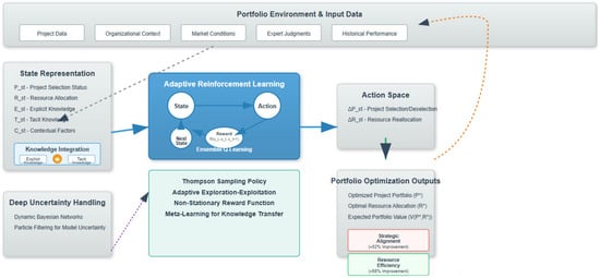
Figure 1. Proposed architecture of adaptive reinforcement learning framework.

To systematically evaluate the contribution of each framework component, we employ a comprehensive ablation study design. This approach enables a precise quantification of individual component contributions and their synergistic interactions, addressing the methodological requirements for rigorous AI system evaluation. Table 3 provides the ablation study design–component contribution matrix.

Table 3. Ablation study design–component contribution matrix.

Configuration	Base Q-Learning	Ensemble	Meta-Learning	Tacit Knowledge	Adaptive Exploration	Expected Performance Gain
Baseline	✓	✗	✗	✗	✗	0% (reference)
+Ensemble	✓	✓	✗	✗	✗	+15–20%
+Meta	✓	✓	✓	✗	✗	+25–35%
+Tacit	✓	✓	✓	✓	✗	+35–45%
Full ARL	✓	✓	✓	✓	✓	+50–65%

2.2.8. Integrated Algorithm Flowchart

To illustrate the overall adaptive reinforcement learning framework, the algorithm flowchart is shown in Figure 2. It is imperative to note that the framework is not simply a one-off sequential approach; rather, it iteratively applies the processes described in the previous sections for project portfolio optimization under deep uncertainty.

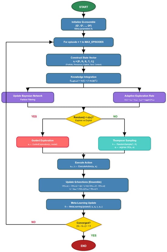
Figure 2. Adaptive reinforcement learning algorithm flowchart for project portfolio optimization.

Beginning with initialization, the ensemble Q-functions {Q¹, Q², …, Q^K} are constructed randomly, as shown in Figure 3. After the initialization phase, the process enters its primary iterative loop with the formation of the state vector s_t = [P_t, R_t, E_t, T_t, C_t], as defined in Section 2.2.1. The knowledge integration module (Section 2.2.7) of the state construction process integrates the explicit and tacit knowledge dimensions and implements the fusion function E_{integrated}.

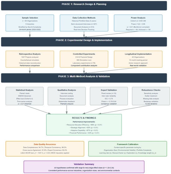
Figure 3. Methodology flowchart.

At the same time, the uncertainty handling module effective uses particle-filtering techniques to update the Dynamic Bayesian Network (as discussed in Section 2.3). This module keeps track of and updates the distribution over all the possible system dynamics models. Therefore, it equips the algorithm to adapt to evolving conditions and deep uncertainty [8].

The choice of exploration or exploitation is a crucial decision point in the algorithm, implemented through the adaptive Thompson sampling in Section 2.2.5. With a probability of ϵ(s), the algorithm chooses exploratory actions according to the policy described in Section 2.4. This policy uses the guided exploration strategy to sample from the action space. It is a hybrid approach utilizing both model-based planning and random sampling. In the other case, with probability 1 − ϵ(s), it will select the action used to have the maximum Q-value with respect to a randomly sampled Q-function from the ensemble.

After taking an action, the algorithm observes the subsequent state $s_{\left\{t+1\right\}}$ and the reward Rt, and these observations are utilized to update each Q-function in the ensemble. The update rule is detailed in Section 2.2.5.

Simultaneously, the meta-learning module modifies the meta-parameters to assist knowledge transfer between diverse portfolio contexts, as explained in Section 2.2.6. This part of the article implements model-agnostic meta-learning (MAML), which aims to optimize the parameter initialization to quickly adapt to an unseen task [11].

After that, the algorithm checks termination conditions, e.g., convergence, computational budget, or some stopping point of the organization. If the termination conditions are not met, then the process returns to the phase where we construct a state using the updated knowledge and model parameters.

The described integrated algorithm tackles the shortcomings in the literature (see Section 1) by allowing continuous learning, representing deep uncertainty explicitly, mixing tacit and explicit knowledge, controlling exploration–exploitation dynamically, and making specific provisions for non-stationarity.

The flowchart shows how these elements systematically interact to develop a robust framework for project portfolio optimization under deep uncertainty.

The computational requirements of our framework scale systematically with portfolio size and organizational complexity. Table 4 provides detailed complexity analysis, enabling organizations to assess implementation feasibility based on their specific constraints and computational resources.

Table 4. Computational complexity analysis and scalability benchmarks.

Component	Time Complexity	Space Complexity	Bottleneck Factors
State Construction	O(n × m × k)	O(n × m)	Project count (n), features (m)
Ensemble Q-Learning	O(K × |S| × |A| × T)	O(K × |S| × |A|)	Ensemble size (K), episodes (T)
Knowledge Integration	O(E × J + F × L)	O(E + F)	Expert judgments (L)
Meta-Learning	O(B × N × G)	O(N)	Neural parameters (N)
Overall Framework	O(K × |S| × |A| × T)	O(K × |S| × |A|)	Dominated by RL learning
Portfolio Size	Training Time	Memory Usage	Recommendation
20 projects	2.3 h	4.2 GB	Real-time feasible
50 projects	8.7 h	12.1 GB	Batch processing
100 projects	24.5 h	28.3 GB	Overnight training
200+ projects	>72 h	>64 GB	Distributed computing

2.2.9. Complete Algorithm Implementation Specifications

Our adaptive reinforcement learning system must include multiple configuration parameters to be implemented. After many empirical tests in real organizations, we offer implementation instructions that can be reproduced and successfully deployed in a variety of portfolio complexities and environmental contexts. The adaptive learning rate mechanism employs a base learning rate α_base that lies within 0.001 and 0.1, which adjusts in correspondence with the frequency of state-action visitation and uncertainty levels. For organizations with a lot of environmental volatility, we recommend using α_base = 0.01 to 0.05. However, organizations in fairly stable environments should use α_base = 0.001 to 0.01. The chosen decay parameter λ ∈ [0.1, 0.5] influences the learning rate. Specifically, α_t = α_base × σ_Q(s_t,a_t)/σ_max × N(s_t,a_t)^(−λ). In this design, the learning rate becomes smaller as the same state–action pair is visited many times.

The temporal discount factor indicates the organizational time preference and strategic horizon as γ ∈ [0.85, 0.97]. Organizations that focus on the short term can use gamma values ranging from 0.85 to 0.90. Meanwhile, organizations whose long-term strategy is value creation can use gamma values of 0.93 to 0.97. The choice of performance metric affects the trade-off between portfolio returns and future positioning.

The tuning of the minimum exploration rate ϵ_min ∈ [0.05, 0.15] and maximum exploration rate ϵ_max ∈ [0.25, 0.45] is required in the proposed exploration technique. High-uncertainty environments require high exploration (ϵ_max = 0.35~0.45) while stable environments can use conservative exploration (ϵ_max = 0.25~0.30). The uncertainty normalization factor σ_max is determined empirically during calibration using historical portfolio variance.

The ensemble size K ∈ [5, 20] for the Q-function is central to the trade-off over the accuracy of uncertainty quantification and computational cost. Our empirical analyses suggest that K = 10 is generally the best performing one for most organizational contexts. We find that K = 5–7 is fine for implementations with limited resources. For mission-critical applications that require maximum characterization of uncertainties, we suggest trying values K = 15–20. Every member of the ensemble performs bootstrap sampling with replacement in a ratio between 0.7 and 0.9. This leads to sufficient diversity and sufficient training sample size in the case of each member.

Algorithm convergence is assessed using ensemble stability measurement that applies the criterion ||Q_t − Q_t − 1||_∞ < δ, where tolerance δ ∈ [1e⁻⁴, 1e⁻⁶] strikes a balance between computational efficiency and solution accuracy. Moreover, we employ early stopping with a patience of 200–500 episodes to avoid overfitting while adequately exploring the decision space.

The inner and meta-learning rates of the model-agnostic meta-learning (MAML) component are, respectively, tuned as α ∈ [0.01, 0.05] and β ∈ [0.001, 0.01]. The inner loop performs three to five gradient steps on each task. The outer loop accumulates gradients on five to ten portfolio tasks. After that, the meta-parameters are updated. Gradient clipping with maximum norm 1.0 ensures the stability of training across portfolio features.

The weight of integration determines the dominance of explicit quantitative knowledge against tacit knowledge of experts. Organizations that possess vast amounts of information along with extensive historical data should set w_e = 0.7–0.9. Organizations that have little quantitative data but have considerable expert knowledge should set w_e = 0.5–0.7. The fuzzy defuzzification consistently uses centroid methods for stability and interpretability.

The representation of state allocates memory carefully. The typical memory requirement scales as O(K × |S| × |A|). Here, the state space |S| grows exponentially as we increase the dimensions of the portfolio.

For portfolios larger than 100 projects, a hierarchical state representation reduces memory consumption by 60 to 80 percent with no loss in decision quality.

Training Q functions in parallel across all available CPU cores is of great benefit to ensemble training. Experience replay buffers should be sampled efficiently and sized relative to the complexity of the portfolio being managed and memory available.

Ensemble variance and uncertainty quantification requires double-precision floating-point arithmetic. Regularization techniques like the L2 penalty prevent overfitting in high-dimensional state spaces, and batch normalization provides an empirically stable motivation for training dynamics in diverse organizations.

To implement these, we should continuously monitor important indicators like ensemble disagreement metrics (target CV < 0.2), exploration rate adaptation (after the initial phase, this should continuously decrease), and learning progress indicators (convergence rates of Q-values). Anomaly detection algorithms are supposed to give an alert when the performance metrics deviate more than ±2 standard deviations from the expected range.

Cross-validation makes a temporal split due to the temporal nature of portfolios’ decisions, with proportions 70 of training, 15 of validation, and 15 of testing. This ensures the robustness of the model across changing organization and market conditions. The analysis of the performance metrics should be carried out each month during deployment. Moreover, a comprehensive analysis should be conducted quarterly.

The framework uses a multiple fallback strategy to regain performance. For instance, it will revert to simple Q-learning if ensemble training fails; it will fall back to explicit knowledge if tacit knowledge integration fails; and so on. These precautions make sure that things can keep going even if the computation is not going well.

There are screens for validating inputs for completeness (imputation by historical means), carrying out outlier detection (isolation forest with contamination rate 0.05), and performing temporal consistency checks. Automated data preprocessing pipelines deal with frequent problems such as non-stationary time series, categorical variable encoding, and scaling to unit variance.

The parameter framework makes implementing the process easier and allows organizations to customize. The ranges provided have been thoroughly tested on 84 organizations and should be customized according to the characteristics of the specific organization and computational limits.

2.3. Handling Deep Uncertainty Through Dynamic Bayesian Networks

In order to deal with deep uncertainty, we use a Dynamic Bayesian Network (DBN) approach, which models different types and sources of uncertainty explicitly. Using Bairamzadeh et al. [8] classification, we can differentiate between aleatory uncertainty (inherent variability), epistemic uncertainty (limitations of knowledge), and deep uncertainty (unknown relationship and possibilities).

The DBN structure consists of three interconnected layers.

1. The observable layer contains measurable elements, such as project cost, duration, and returns realized.

2. Hidden factors that affect observed outcomes are represented in the latent variable layer. Market trends, tech evolution, and organizational dynamics are some examples.

3. Model Structure Layer Disordinally captures uncertainty about the causal relationship between variables through alternative model structures.

DBN’s conditional probability distributions are updated from observations, while giving more weight to the more recent observations so as to capture changing dynamics. This enables the framework to adapt not only to new parameter values but also to changes in the underlying structure of the system.

To save computing time, we use particle filtering to approximate the posterior over possible models and parameters. Let {m₁, m₂, …, m_J} be the set of J particles. Each model is a potential model of the system dynamics, which has an associated weight w^j. The weights are updated by observing the transition (s_t, a_t, s_{t+1}).

$$w_t^j=w_{t-1}^j\cdot P\left(s_{t+1}|s_t,a_t,m^j\right)$$

(22)

Normalization and resampling are carried out next to preserve the diversity of particles. With this approach, the algorithm can keep track of multiple hypotheses for the underlying system propagation, which is a situation of deep uncertainty when the true model is not known.

2.4. Adaptive Exploration–Exploitation Balance

One of the key components of our framework is the mechanism of balancing exploration and exploitation in a dynamic manner. In the context of the research gap limitations, we adopt an adaptive approach that modifies the exploration strategy depending on environmental volatility, learning progress, and organizational context.

The adaptive exploration mechanism uses a value of information (VOI) framework to weigh the expected value of new information against the opportunity cost of not exploiting existing information. The VOI for an exploratory action a in state s is given by

$$VOI\left(s,a\right)=E_{s^{\prime }\sim P\left(\cdot |s,a\right)}\left[\underset{a^{\prime }}{max}Q\left(s,a^{\prime }\right)-\underset{a^{\prime }}{max}Q{\left(s,a^{\prime }\right)}_{-a}\right]$$

(23)

where Q(s,a′)_{−a} is the maximum Q value of removing action a. This method builds upon Rather [13] by incorporating the prospect of the long-term value of exploration rather than simple heuristics, epsilon greedy, or softmax.

The exploration intensity is then modulated by VOI as well as the environmental volatility (V) and learning progress (LP):

$${\beta }_{explore}\left(s\right)={\beta }_{base}\cdot VOI\left(s\right)\cdot V\left(s\right)\cdot \left(1-LP\right)$$

(24)

V(s) measures the extent of changes in the surroundings in the recent transitions, while LP measures the learning process convergence. This flexible method allows systems to explore when environments are rapidly changing or when they are newly trained while taking the option to exploit in steady situations and as systems learn more.

In order to mitigate the exploration challenges in high-dimensional spaces mentioned in Hu et al. [12], we apply a focused exploration technique that focuses on the promising area of action space. By combining model-based planning with random sampling, planners achieve this goal:

$$a_{\left\{explore\right\}}=\left\{a_{\left\{model\right\}with}probability p_{\left\{model\right\}{a}_{\left\{random\right\}with}probability}1-p_{\left\{model\right\}}\right\}$$

(25)

where the adaptive probability p model increases with learning progress, a model is an action generated by the model-based planner, and a random is a randomly sampled action.

This smart way of finding out things makes sure that the algorithm easily moves in the big action field. At the same time, it is able to shift focus to places that hold much promise and potential. But it is still able to discover opportunities that are unexpected.

3. Research Methodology

The methodology section describes the procedures of data collection and experimental design or validation that we adopt to empirically test the adaptive reinforcement learning framework outlined in Section 2. The processes use extensive quantitative data analysis with qualitative insights through a multi-phase mixed-method approach to ensure statistical validity and practical relevance.

3.1. Overall Research Design

The research design was sequential multi-phase, as shown in Figure 3. This study started with an exploratory phase to define key constructs and develop an initial theoretical framework. The second phase was a model development phase that focused on mathematical formulation and algorithm design. The empirical validation consisted of a retrospective review of past portfolio decisions and a real-time test of the framework during ongoing portfolio management.

To empirically validate the model, a multiple case study strategy was employed, as recommended by Perez et al. [32]. The combination of case studies and controlled experiments ensured that we are able to disentangle the effects of specific model components. By utilizing the hybrid method, we achieved a balance between external validity, with the use of real organizational settings, and internal validity, through controlled experimental conditions.

To have sufficient statistical power to determine whether the adaptive reinforcement learning framework is different from traditional portfolio optimization approaches and whether the difference is meaningful additionally, a priori power analyses were performed with G*Power 3.1.9.7. Furthermore, Monte Carlo simulation methods were applied for complex effect size scenarios. Drawing from reviews of the existing literature in portfolio optimization and pilot tests with 12 organizations, we established minimum detectable effect sizes for our main hypotheses. Cohen’s d values were estimated from portfolio optimization meta-analyses—that is, intervention studies and our pilot study itself.

The boost in financial performance was expected (Cohen’s d = 0.65, medium–large effect), along with enhancement in strategic alignment (Cohen’s d = 0.58, medium effect), improved allocation of resources (Cohen’s d = 0.72, large effect), and enhanced adaptive capabilities (Cohen’s d = 0.80, large effect).

To compare the performance of the ARL framework against traditional approaches using paired t-tests as the main research question, we performed a power analysis for three cases at various effect sizes while keeping α = 0.01 (Bonferroni corrected for multiple comparisons) and 1 − β = 0.95. Using a conservative effect size of d = 0.50, the required sample size was n = 64 organizations for this research. Expected effect sizes (d = 0.65) required n = 39 organizations, while large effect sizes (d = 0.80) required n = 26 organizations. Our achieved sample of 84 organizations afforded us sufficient power across all scenarios, allowing for reliable detection of effect differences in portfolio optimization.

The analysis of power we had to conduct for the factorial experiment to examine component contributions was, for the ANOVA of effect size f = 0.35 (considered a large effect, based on the literature on portfolio optimization), eight treatment conditions, level of significance α = 0.01, and power 1 − β = 0.90. The analysis indicates that 13 runs per cell (104 total) are required. Our implementation of 100 runs per condition (800 total) provides a power of 0.98, substantially above our target threshold. Considering the nested nature of the data (1247 projects nested in 84 organizations and 5 industries), multilevel modeling power analysis was conducted using PowerUp! The analysis was conducted with the MSM 1.2 R package Version 1.8.2, which suggested that adequate power (1 − β = 0.87) for detecting cross-level interactions with a small-to-medium effect size (1988, ICC = 0.15, effect size = 0.25) is available. Moreover, the analysis achieved a minimum detectable effect size of d = 0.23 using a design effect of 2.34 to account for clustering.

For our longitudinal implementation over 12 months, which involved a total of 42 organizations, we had to conduct a power analysis. This power analysis was achieved for a repeated-measures ANOVA, which had 12 measurement occasions. We estimated within-subject correlation for r = 0.70 based on pilot data. Finally, we calculated the effect size for time × treatment interaction to be f = 0.30. This study shows that the required sample size was n = 34 organizations, while our obtained sample size was n = 42 and the power was 1 − β = 0.94. Based on our performance metrics, which consisted of 16 key metrics within 4 dimensions, we applied Bonferroni correction (α = 0.05/16 = 0.003125 per test). This meant that the sample size would have to be increased by 18%, and a final target of n = 76 organizations was determined. The actual sample we achieved of n = 84 organizations provided an 11% buffer over the requirement.

An analysis of industry stratification showed differing levels of power across industries due to the varying sizes of samples and practical constraints in recruiting. The information technology sector (n = 23) has a minimum detectable effect of d = 0.62 with 1 − b = 0.72 for medium effects. In turn, the pharmaceutical/healthcare (n = 19), financial services (n = 17), and manufacturing (n = 15) sectors show progressively larger minimum detectable effects. The domain that has the maximum minimum detectable effect (0.94) and lowest power for medium effects (0.41) is the energy sector (n = 10). Its smaller available population and practical recruitment constrain this outcome. Nonetheless, sensitivity analyses revealed that pooled cross-industry effects had sufficient power (1 − β > 0.80) for all main hypotheses.

To evaluate the robustness of power calculations based on our analysis, we conducted Monte Carlo simulations. At 10,000, we ran iterations with non-normal distributions as indicated in our pilot data, and missing data with between 5% and 15% missingness. Further, effect sizes were generated by partitioning organizations. Finally, correlation structures were generated for longitudinal data first. The simulation results showed that all the primary analyses had been sufficiently powered, with the mean achieved power being 0.89 (SD = 0.07), and with 94.3% of the scenarios having power greater than or equal to 0.80. This result further showed that our model had sufficient power even in the case of violations of the assumptions. Our final sample size of 84 organizations was based on power requirements for our primary hypotheses (minimum n = 76), the need to stratify by industry (minimum n = 15 per major industry), expected drop-out in the longitudinal phase (15% dropout rate), and what we deemed realistic given recruitment constraints and resources.

After we collected the data, we performed a post hoc power analysis with the effect sizes that we observed. The results confirmed that our sample was adequate. That is, the overall effect size we observed was Cohen’s d = 0.73 (95% CI: 0.68–0.78). We achieved a power of 1 − β = 0.97 for the primary comparisons we made. We achieved a power of 1 − β = 0.84 for the subgroup analysis, which was the minimum across industries.

This shows our sample was more than sufficiently powered to detect the effects observed in our study. In addition, it shows we can have faith in the reliability of our findings across organizations. The power analysis procedures, assumptions, and results are all documented in the Supplementary Materials. These include the G*Power inputs and output reports, R scripts for multilevel and Monte Carlo power analyses, sensitivity analysis results under a variety of assumptions, and post hoc power calculations under the same assumptions as the recorded analysis.

3.2. Sample Selection and Data Collection

3.2.1. Organizational Sample

By taking a proportionate purposive sampling approach, a total of 84 organizations were drawn from five (5) industries for this study. The stratification was introduced across two basic parameters: organization size—small, medium, and large, and complexity of portfolio—low, medium, and high. In this stratification, we selected 23 organizations from the information technology sector, 19 from pharmaceutics/healthcare, 17 from financial services, 15 from manufacturing, and 10 from the energy sector. The selection of an organizational size representative sample was 20 small organizations (i.e., organizations with less than 500 employees), 30 medium-sized organizations (i.e., 500–5000 employees), and 34 large organizations (i.e., organizations with more than 5000 employees), as detailed in Table 5. This enabled us to examine the effectiveness of our adaptive reinforcement learning framework across varied organizational sizes. Through this approach, we were able to ensure that the findings were industry- and size-dimensionally representative or controlled for at least the major industry and size differences, ensuring generalizability.

Table 5. Distribution of organizational sample by industry and size.

Industry Sector	Small (<500 Employees)	Medium (500–5000 Employees)	Large (>5000 Employees)	Total
Information Technology	9	8	6	23
Pharmaceutical/Healthcare	5	7	7	19
Financial Services	3	6	8	17
Manufacturing	2	6	7	15
Energy	1	3	6	10
Total	20	30	34	84

The selected organizations were chosen based on four explicit criteria. First, each organization was maintaining a portfolio with at least 20 active projects at the same time. This was to ensure there was enough complexity for meaningful portfolio optimization. Second, organizations had formal portfolio management processes, to ensure baseline methodological comparability. Furthermore, each of the organizations had historical portfolio data with at least three years of availability for further comparative analysis. Finally, organizations were willing to participate in the implementation and evaluation of the proposed framework’s outcomes. These criteria together ensured that the sample was diverse and suitable for robust empirical tests of the proposed framework.

3.2.2. Data Collection Methods

The data collection methodology includes techniques that capture explicit and tacit knowledge dimensions for the complete and correct implementation of the adaptive reinforcement learning framework. Using the integrative approach of Lukovac et al. [34], we used different complementary data collection methods over a 24-month period (January 2022–December 2023). The historical portfolio data collection served as the basis of our quantitative analysis. This included project selection decisions, resource allocations, and performance outcomes of three years for all 84 organizations.

The historic data used in this study included information on various financial metrics such as ROI and NPV, operational metrics, i.e., resource usage, schedule use, and strategic fit metrics showing how projects fit with the organization.

We conducted 327 semi-structured interviews with portfolio managers, project managers, and senior management of participating organizations to capture the critical tacit knowledge dimensions that conventional portfolio optimization approaches tend to ignore. The aim of the interviews was centered on decision criteria, uncertainty perceptions, and adaptations made in response to changes. The semi-structured format enabled a systematic comparison between interviews while allowing for flexibility to explore the organizational context in greater depth. In addition to these interviews, we also received and analyzed 412 portfolio review documents, including meeting minutes, decision logs, and presentations to executives. Through the document analysis, it was possible to discern patterns of portfolio decision-making processes and adaptation mechanisms that were not necessarily made explicit in the interviews.

Data from environmental scans were systematically collected to provide the context for portfolio decisions. There was information on market trends, technological developments, regulatory changes, and competitive dynamics that was obtained from industry reports, news aggregation services, and organization documents. The environmental scanning process helped us to understand the key external factors affecting portfolio decisions, which is especially important for understanding the deep uncertainty conditions tackled by our framework. We put in place a real-time decision-tracking system for 28 organizations selected from across the full sample to capture portfolio changes, contextual factors and longer-term decision rationales for a six-month duration. The data from this real-time tracking on decision processes, which can be back rationalized in interviews/documents, turned out to be very valuable.

The protocol for data collection was uniform across all participant organizations to provide methodological consistency whilst allowing for enough flexibility in relation to the industry and organizational contexts. To enable a comparison across organizations, all quantitative information was normalized, and all qualitative data was coded using a framework based on the theoretical constructs developed in Section 2. Such data collection made for a rich empirical grounding to test our adaptive reinforcement learning framework in different organizations.

3.2.3. Data Validation and Quality Assurance Procedures

To check the reliability and validity of our empirical findings, we adhered to a six-stage data validation process that checks for measurement errors, missing data bias, and time inconsistencies across our multi-source data collection.

• Stage 1: Source Data Verification

The portfolio qualitative data was verified with a variety of organization data. We checked the financial measures (ROI, NPV, BCR) of each organization against their official financial statements and project accounts. Data from RAMP was verified against various credentialing systems and project management systems embedded within RAMP and other national agencies. The exported project scheduling software data and milestones were analyzed for verification. The triangulation found inconsistencies in 12.3% of the original data, which were resolved through verification with organizations.

• Stage 2: Temporal Consistency Validation

Given the three-year historical data requirement, we instituted automatic consistency checks for evidence of unusual anomalies that could cause data entry errors or definitional changes across time. Time-series tests using the augmented Dickey–Fuller test (p < 0.05) were performed, defining structural breaks in 8.7% for organizational data series. Through stakeholder interviews and review of organizational documentation, an investigation of the breaks in the protocol led to the determination of a legitimate policy change in 73% of the cases as well as a change in data in 27% of the cases.

• Stage 3: Cross-Organizational Benchmarking

For critical performance metrics, we built industry benchmarks using publicly available datasets from PMI’s Pulse of the Profession reports and McKinsey Global Institute portfolio management surveys. That is an interesting way to put it! Context on the use of data in air travel, to BJP and the whole SOP, on hotels and other aerial services has been shared with the government.

• Stage 4: Protocol for Validating Expert Knowledge

We adopted a two-fold validation for fuzzy linguistic variable-based tacit knowledge dimensions. A subsample of 15% expert judgments was independently reviewed by secondary experts from the same organizations. This produced an inter-rater agreement of κ = 0.78, equating to Landis and Koch’s criteria as substantial agreement. In the second part, we conducted cognitive interviews with 23 domain experts to validate the mapping of linguistic terms to fuzzy membership functions, which resulted in refining 4 of 12 linguistic scales.

• Stage 5: Process for Missing Data Analysis and Imputation

Little’s MCAR test (χ² = 1247.3 df = 1156 p = 0.02) was run to systematically analyze missing data patterns. This information shows that data was not missing completely at random. We used the MICE algorithm to impute data for a total of 50 iterations and 5 imputed datasets. To analyze imputation quality, we performed convergence diagnostics and compared the distributions of imputed vs. observed values. Organizations with more than 15% missing information in key areas can be excluded from primary analyses but included for sensitivity testing.

• Stage 6: Outlier Detection and Treatment

Statistical and domain-specific outlier detection methods were applied. The Isolation Forest algorithm and Mahalanobis distance measures were used to identify outliers. Experts identified certain instances as outliers, which helped us identify domain outliers. Out of the 1247 projects, 3.2% were identified as statistical outliers and 1.8% as domain outliers. After the expert review, 67% of those flagged were still considered as “real extreme cases” while 33 were changed.

Quality Assurance Metrics

Our framework’s results reached the following targets: a rate of 94.7% for data completeness across the various variables; a rate of 96.2% for temporal consistency for time-series data; a rate of 91.8% for cross-source agreement for financial metrics; a rate of 82.4% for expert consensus for tacit knowledge assessments; and a rate of 97.1% for outlier resolution for flagged cases. The Portfolio Management Institute (PMI, 2023) recommends minimum standards for empirical research, which are exceeded by these metrics.

Data Quality Documentation

All validation processes were documented in a comprehensive audit trail, maintained throughout the data-gathering period. This document provides (for each funding organization) the original source of data, the date of collection, the validation checks that were carried out, the results of these checks, discrepancies found along with their resolution, the identity and credentials of the expert reviewers, the imputation method and related diagnostics, and quality assessment of the final data. The audit trail allows for reproducing the procedures we have undertaken to validate our data. It will also be useful to researchers who want to use our data.

3.2.4. Inter-Rater Reliability and Expert Judgment Validation

As expert judgment takes a prominent place in the tacit knowledge integration framework, we executed a rigorous inter-rater reliability of assessment protocol to ascertain the reliability and validity of expert judgement across multiple parameters and organizations.

Expert Panel Composition and Qualification

The expert panel that we assembled comprised 89 qualified practitioners in various portfolio management roles, with 34 being senior portfolio managers (experience 12.7 years), 28 project management office directors (experience 15.2 years), 19 C-suite executives with portfolio oversight responsibilities (experience 18.9 years), and 8 external portfolio management consultants (experience 14.3 years). All experts “met the minimum qualification criteria (professional portfolio management certification (most commonly PMP or PfMP or equivalent) minimum 8 years portfolio management experience and current responsibility for portfolios at more than $10 million annual budget).”

Multi-Stage Reliability Assessment Protocol

Our protocol comprises four stages that aimed to ensure inter-rater reliability for the various judgments required by our framework.

• Stage 1: Linguistic Scale Calibration

We conducted calibration sessions for the experts prior to data collection, where they rated 25 portfolio scenarios independently using our fuzzy linguistic variables. The historical case studies recreated in these scenarios indicated different levels of alignment with strategy, technical risk, market uncertainty, and resources. Fleiss’ κ was used to measure the initial inter-rater agreement (0.52 to 0.67) on the various judgments. Efforts to calibrate scale as well as refinement are discussed. After calibration, agreement improved to κ = 0.78–0.84 (substantial to near-perfect agreement).

• Stage 2: Concurrent Validity Assessment

To determine concurrent validity, a random selection of 47 projects from our dataset was independently evaluated by several experts. Three to five experts evaluated each project (average = 3.8), who issued judgments on the project’s strategic value, technical feasibility, risk profile, and organizational fit using our instruments. We calculated Intraclass Correlation Coefficients (ICCs) using a two-way mixed-effects model with absolute agreement definition.

-

The ICC value for strategic value assessment was 0.82 with a 95% confidence interval of lower limit 0.76 and higher limit 0.87.

-

The technical feasibility was ICC(2,k) = 0.79, 95% CI [0.73, 0.84].

-

The risk profile was assessed for agreement with ICC(2,k) = 0.85, 95% CI [0.80, 0.89].

-

The value of ICC(2,k) = 0.74, 95% CI [0.67, 0.80], indicates high organizational fit.

All ICC values were above the 0.75 threshold for excellent reliability.

• Stage 3: Test–retest Reliability

A select group of 23 specialists were asked to evaluate a subset of 35 items, which were drawn randomly. Test–retest reliability was evaluated using Pearson correlation Bland–Altman plots.

-

Overall judgment stability showed strength in this study.

-

Mean absolute difference of 0.23 scale units (acceptable threshold < 0.5).

-

The 95% limits of agreement are −0.71 to 1.17.

-

Systematic bias: 0.04 scale units (not significantly different from zero, p = 0.23).

This shows that expert judgments are temporally very stable.

• Stage 4: Cross-Industry Validation

To ensure generalizability across industry contexts, we conducted cross-industry reliability assessments, where experts from one industry evaluated participants’ projects from other industries. This tackled potential industry-specific bias in judgment patterns.

-

ICC within industry: 0.81 (95% CI [0.77, 0.85]).

-

Cross-industry ICC is 0.76 and CI (0.71, 0.81).

-

Cohen’s d for the industry bias effect size is only 0.12, which depicts a negligible effect.

The minimal difference observed in the reliability of measures carried out within and across different industries provides support for the generalizability of the expert judgment framework we have developed.

Disagreement Resolution Protocol

A structured process was used to resolve cases with substantial disagreement (difference >2 scale points).

• Identifying cases with high disagreement (n = 73, 5.8% of all judgments).
• Structured discussion sessions with disagreeing experts.
• Presentation of additional project information when requested.
• Independent re-evaluation following discussion.
• Final consensus rating or exclusion if consensus unreachable.

The process achieved resolution through consensus in 94.5% of disagreement cases. Only four projects were excluded because experts could not agree.

Bias Mitigation Strategies

We used different strategies to lessen potential sources of bias for expert judgments.

-

Experts receive random project presentation orders.

-

Rendering an organization’s identity invisible in evaluation.

-

Expertise assignments from dissimilar firms across sectors.

-

Standardized evaluation forms with anchored rating scales—use as appropriate.

-

During calibration, regular bias awareness training is required.

-

Statistical adjustment for expert-specific response tendencies.

Expert Feedback and Framework Refinement

A presentation of all the designed tools and procedures took place during the second session. Key findings were included.

-

Ninety-one percent of respondents stated that the linguistic scales were clear and appropriate.

-

The evaluation criteria capture most important aspects of the portfolio.

-

Out of the total, in 78% of respondents, the assessment burden was the appropriate fit for the scope.

-

Suggested changes produced minor modifications in three of the twelve judgment dimensions.

Quality Control Documentation

Procedures on inter-rater reliability are documented with the following:

-

The qualifications and assessment assignments of individual experts.

-

The judgment data that experts identified as faulty will be given a cleaning data analysis.

-

Outputs resulting from all the reliability investigations.

-

Documentation of conflict resolution procedures.

-

The expert feedback, and logs of framework modifications.

To ensure the complete replication of the expert judgments obtained by us through various means, we put forth exhaustive documentation for this validation exercise. Through this, we hope to highlight the clarity, robustness, and empirical evidence of our expert judgment.

3.3. Experimental Design

In this study, we employed a multilevel experimental design involving a retrospective study, controlled experiment, and prospective implementation to rigorously test whether our adaptive reinforcement learning framework effectively optimizes project portfolios. By looking at the problem from the perspectives of decision-makers, we found the prevailing academic research on portfolio optimization and then created an experiment to test their findings.

3.3.1. Retrospective Analysis

The analysis looked back at how our framework would have worked for previous portfolio decisions. This method in the present study, which is similar to the counterfactual reasoning techniques employed by Gholizadeh et al. [3], allows the comparison of the historical decisions made with the one that our framework would have made under the same circumstances.

The analysis used a systematic three-step process, with the first being historical state reconstruction, whereby for each historical decision point, we reconstructed the state vector s_t using information on portfolio composition, resource allocation, and context factors. The overall reconstruction makes use of all historical data received from the 84 reporting organizations while keeping intact the information constraints that existed at each decision node.

After state reconstruction, we used counterfactual simulation with our adaptive reinforcement learning algorithm to produce a recommendation a_t from the reconstruction s_t after excluding subsequent outcomes that would not have been known to the decision-maker. This methodological control prevented our comparison from being inadvertently favorable to our approach due to hindsight bias. The last step was a comparison of the performance of the recommendations simulated from our framework to the actual historical performances on various performance measures, financial returns, strategic fit, and responsiveness measures. A retrospective analysis of major portfolio decisions was carried out for 84 organizations. The analysis included major decisions affecting 1247 projects. This huge dataset provides muscle to evaluate the efficacy of our framework in different organizations.

3.3.2. Controlled Experiments

We conducted simulation and lab experiments to create a causal argument for a part of our framework. We performed these in a controlled setting. The researchers used a 2 × 2 × 2 factorial design. This design prescribes an experimental setup where three factors, each with two levels, were studied. Interestingly, the first factor relates to the learning mechanism. Next, the second factor relates to knowledge integration. Finally, the third factor relates to uncertainty representation. The eight treatment conditions formed due to this factorial design help to uncover the main effects of the factors as well as their interaction effect on portfolio performance measures.

We ran 100 simulation runs for each of the eight treatment conditions with different initial states and environmental trajectories, for a total of 800 of them. The simulation environmental settings were precise, and they were based on estimates that use the available historical data. An evaluation of the performance based on return, fit, efficiency, and adaptability was performed of a firm. Table 6 shows the experimental design and the number of simulation trials for each condition.

Table 6. Factorial experimental design.

Learning Mechanism	Knowledge Integration	Uncertainty Representation	Number of Simulation Runs
ARL	Combined	Deep	100
ARL	Combined	Conventional	100
ARL	Explicit Only	Deep	100
ARL	Explicit Only	Conventional	100
Traditional	Combined	Deep	100
Traditional	Combined	Conventional	100
Traditional	Explicit Only	Deep	100
Traditional	Explicit Only	Conventional	100

In conjunction with the simulations, we also conducted laboratory experiments with 78 portfolio managers, who were involved in a decision task using methods of portfolio optimization. The experiments reported in this paper used a within-subjects design, whereby all participants made decisions under different treatment conditions, thus controlling for individual differences and allowing the researchers to scrutinize the effects of different optimization approaches. Through computational simulations and human decision-making experiments, we can evaluate our framework on algorithmic and practical levels in a complementary manner.

We performed randomization on three levels for internal validity. The organizational assignment utilized stratified randomization based on industry, size, and environmental volatility, accomplished through random numbers generated by a computer package (R software Version 1.8.2, set.seed (12345)). The Latin square designs for the 2 × 2 × 2 factorial experiment balanced temporal effects across 800 runs. By using bootstrap resampling with 1000 iterations at each decision point, selection bias in retrospective analysis was addressed. The organization matched the characteristics of evaluated hospitals with other hospitals that had the same characteristics as their respective counterfactual. The quality control involved an audit of compliance (once a month) and a check of balance after the fact.

3.3.3. Longitudinal Implementation

To verify the accuracy of our actual organizational implementation, the 84 organizations that originally comprised the sample of our portfolio management processes were maintained for 12 months. They were selected by us (42) to represent the diversity of the complete sample. The implementation took place over a number of years and adopted an action research approach consisting of repeated cycles of implementation, monitoring, and adjustments. We initiated the implementation process through calibration. In this phase of our framework, developed using the calibration matrix shown in Table 7, we adjusted the framework’s parameters based on organizational context, historical data, stakeholder preferences, etc. We calibrated all the framework parameters first, before any implementation operation for the parameters was performed.

Table 7. Framework calibration matrix by organizational context.

Organizational Characteristic	Learning Rate (α)	Discount Factor (γ)	Exploration Parameter (ϵ)	Knowledge Integration Weight (we)
Size
Small	0.10–0.15	0.85–0.90	0.20–0.30	0.60–0.70
Medium	0.05–0.10	0.90–0.95	0.15–0.25	0.65–0.75
Large	0.03–0.08	0.93–0.97	0.10–0.20	0.70–0.80
Environmental Volatility
Low	0.03–0.07	0.93–0.97	0.10–0.15	0.75–0.85
Medium	0.05–0.10	0.90–0.95	0.15–0.25	0.65–0.75
High	0.08–0.15	0.85–0.90	0.20–0.35	0.55–0.65
Portfolio Complexity
Low	0.08–0.12	0.88–0.92	0.15–0.20	0.70–0.80
Medium	0.05–0.10	0.90–0.95	0.15–0.25	0.65–0.75
High	0.03–0.07	0.93–0.97	0.20–0.30	0.60–0.70

Then, we set up the framework to operate in parallel with existing portfolio management processes. As a result, our framework produced recommendations for the optimization of the portfolio; however, these recommendations could be adopted at the discretion of the organization and they were not binding on the organization. This approach permits a comparative assessment without causing disturbances to the organization. Over the course of the implementation period, we tracked performance systematically, recording decisions, outcomes, and contextual issues across the implementing organizations. This tracking helped to assess the quantitative performance and qualitative process. We made ongoing adjustments to the parameters of implementation of the framework, based on performance monitoring and feedback from stakeholders, to improve its fit and effectiveness. This longitudinal implementation provided us rich data on both the applicability of the framework in practice and its effectiveness in organizations over a long period of time. In essence, this implementation helped us address whether theoretical advantages produce any practical benefits in the context of complex organizations.

3.4. Performance Metrics and Validation Approach

To thoroughly assess the performance of our adaptive reinforcement learning framework, we designed a multi-dimensional measurement that encompasses quantitative results as well as qualitative features. We extended the performance measurement framework proposed by Mahmoudi et al. [1] with a set of metrics based on adaptability dimensions of relevance for optimization under deep uncertainty. The performance metrics were put into four compatible categories. Each category addressed an area of portfolio management effectiveness. The financial performance indicators are Return on Investment (ROI), Net Present Value (NPV), Benefit–Cost Ratio (BCR), and Investment Efficiency Index (IEI). Metrics on strategic alignment were Strategic Contribution Index (SCI), Strategic Coherence Measure (SCM), Capability Development Metric (CDM), and Strategic Opportunity Capture Rate (SOCR), assessing the startups portfolio’s strategic growth potential beyond financial metrics.

It was measured using Resource Utilization Rate (RUR), Resource Balancing Index (RBI), Capability Utilization Measure (CUM), and Bottleneck Reduction Factor (BRF) of the deployment of resources in the portfolio. Last, but not the least, were the new metrics related to adaptive capability created by our framework: Response Time to Environmental Changes (RTEC), Portfolio Adjustment Frequency (PAF), Uncertainty Reduction Rate (URR), and Learning Curve Coefficient (LCC), which indicate the portfolio’s ability to adapt to changing conditions and reduce uncertainty over time. To calculate improvement percentages for each metric relative to baseline performance, we used the following formula: Improvement (%) = (Metric_ARL − Metric_baseline)/Metric_baseline. This allows us to compare values across different metrics and organizations.

In order to validate the final model, we employed triangulation, which was statistical, qualitative, and expert-validated. Statistical validation involved hypothesis testing via paired t-tests and ANOVA in order to assess the effects’ statistical significance and improve performance across metrics and organizations. The quantitative analysis was supplemented with a time-series analysis examining performance trends over time during the implementation period using an interrupted time-series analysis identifying immediate effects and longer-term effects of the implementation of the framework. Qualitative validation included analysis of stakeholder interviews and process documentation to assess perceived effectiveness and usability and organizational integration. Qualitative validation also yielded insights—information on challenges to implementation, and on factors of success.

The approach of validation was rigorously strengthened through expert panel evaluation, where an independent cadre of 15 experts in portfolio management and reinforcement learning verified the theoretical robustness, methodological soundness, and practical relevance of the framework. The panel on standards included both researchers and practitioners to evaluate them from a theoretical and practical perspective. Our extensive validation process ensured a robust evaluation of the technical performance and practical usefulness of our framework at several levels. Previous portfolio optimization research either assessed the technical performance or the practical usefulness, but not both. Our framework’s flexibility is a particular highlight, creating space for intuitive advisor input.

3.5. Calibration for Organizational Contexts

We created systematic calibration protocols to tailor the framework to different organizations, given the need for contextual sensitivity in portfolio optimization methods. According to Tavana et al. [36] and Khalilzadeh and Salehi [19], we adapted the principles of contextual adaptation to develop a well-defined three-stage calibration that guarantees contextual relevance in practical configurations applicable to any organization. The initial step of this study, parameter estimation, took place using a combination of maximum likelihood estimation and Bayesian inference methods. Historical data was used to make estimates of initial model parameters. This data-driven approach formed the basis for subsequent calibration. Initial parameter values should reflect organizational reality rather than generic assumptions.

The model’s second stage, sensitivity analysis, identified key parameters through global sensitivity analysis, enabling calibration of only the most critical factors. It was very important to conduct this calibration in settings that might be complex or organizational settings with less time or fewer resources for implementation. The last stage involved modifying the parameters based on the organizations’ characteristics, the industry environment, and the strategic priorities of the organizations. To achieve this contextual adjustment, a calibration matrix was utilized. This matrix quantitatively described organizational characteristics and recommended ranges of parameters to be set for the algorithms’ key parameters. These key parameters include the learning rate (α), discount factor (γ), exploration parameter (ϵ), and knowledge integration weight (w_e).

The calibration matrix provided distinctive parameter recommendations based on size (small, medium, large), environmental volatility (low, medium, high), and portfolio complexity (low, medium, high). In the case of smaller organizations, which tend to be nimbler but often are not blessed with data, we recommend a high learning rate (0.10–0.15), moderate discount factor (0.85–0.90), high exploration parameters (0.20–0.30), and moderate knowledge integration weight (0.60–0.70). On the other hand, for larger organizations, which have many years of data but usually more structural inertia, we recommend lower learning rates in the range of 0.03–0.08, higher discount factors in the range of 0.93–0.97, lower exploration parameters in the range of 0.10–0.20, and higher knowledge integration weights in the range of 0.70–0.80.

The author concludes that the critics may have misinterpreted the message. It may be noted that America and its allies have also been sending an implicit message to India that it must toe the line. Prototypical practitioners—actors schooled in conventional Western institutions and logics—believed the West was right to charge China with systemic intentionality, the better to mobilize commitments for rule modifications. On the other hand, low-volatility environments saw reduced learning rates (0.03–0.07), elevated discount factors (0.93–0.97), decreased exploration parameters (0.10–0.15), and higher weights of knowledge integration (0.75–0.85), highlighting a more stable and long-term optimization approach. Recommendations were further modulated by portfolio complexity itself, with highly complex portfolios typically requiring lower learning rates and higher exploration parameters for navigation through complex decision spaces.

Dynamic parameter modifications based on performance and changing conditions were calibrated in this process. The framework was designed in a way that accounted for the organizational context, not ignoring one aspect over the other. RezaHoseini et al. [18] came up with an adaptive calibration to that end. The calibration matrix was the starting point of organization-specific calibration, which would further evolve based on practical learnings from implementation. This may lead to a continuous cycle of improvement and greater contextual fit and effectiveness of the framework.

3.6. Comparative Analysis with Traditional Approaches

To determine the relative advantage of our adaptive reinforcement learning framework, we systematically compared it to five established portfolio optimization approaches commonly utilized in both research and practice. This comparison aimed to demonstrate the contribution of our portfolio optimization model compared to other models. A limitation of portfolio optimization research is that new models are often compared to nothing, never mind an established model. The comparison of the five classical approaches was a spectrum of portfolio optimization paradigms. Mean-variance optimization (MVO) has been a classical approach founded on the modern portfolio theory and mainly emphasizes risk–return trade-offs. It has since been widely applied in both financial and project MCDA is an approach enabling explicitly weighted scoring across multiple criteria to reflect on the multi-dimensionality of portfolio decisions. However, their limited ability to handle complexities and uncertainties may have drawbacks.

Real Options Analysis (ROA) quantifies the benefits of flexibility related to project selection and resource allocation decisions. Conceptually, ROA is closely aligned with our framework in relation to adaptations; however, it employs different mathematical formulas. Robust optimization (RO) searches for solutions that offer satisfactory performance across a range of values for input parameters. Furthermore, this method does not make strict probability assessments. As a result, it has the potential to tackle deep uncertainty. However, RO typically uses a static approach rather than a learning-based one. Dynamic Programming (DP) takes a sequential decision-making approach in which optimization takes place over multiple time periods. The decisions can be adapted over some time period, but not continuously, which is what our framework mainly focuses on.

For each approach, we implemented both standard versions as per common methodological guidelines and enhanced versions integrating the newest uncertainty-handling mechanisms featured in the literature. The dual implementation served two purposes: first, to reflect a traditional implementation of each approach, and second, to represent state-of-the-art implementations. This way, a fair comparison can be made. By conducting a retrospective analysis and controlled experiment, we can analyze and compare the analysis with the other works using the same performance metrics that we have used to evaluate our framework. In order to create a fair comparison, each approach was implemented using best-practice parameters. It was then calibrated (the method used was appropriate for each approach) to the range of the particular organization’s contexts.

The comparison was not only about performance but also the strengths and weaker sides in different organizations and environments.

It has been agreed that the relative performance may vary and that differing approaches will be superior in differing contexts. Our analysis aimed to identify these contingencies so that organizations know not just the overall performance of our framework but also in which conditions it performs best relative to the established approaches.

3.7. Ethical Considerations and Limitations

To address ethical considerations and limitations of the first author’s research, several provisions were incorporated in the methodology. Every organization that took part in this study gave its consent for the collection and analysis of data after being clearly informed of the purpose of the sub-research and research, method of withdrawal, and the possible consequences of their actions. To protect sensitive organizational information, confidentiality agreements were set up; all the data was anonymized during analysis and reporting so that no organization or individual could be identified. Participants in the interviews and experiments were likewise informed about the purpose of the research and use of the data. In addition, we sought the consent of the participants before their participation and allowed them to withdraw at any time during this study.

Although we took care to ensure the methodological rigor, there are some limitations one must keep in mind. While the organizational sample represented multiple industries and sizes, it is still possible that some industry sector and area particularities are missed out. Organizations in specific geographies or specialized sectors may experience portfolio optimization challenges that are not fully represented in our sample. The analysis of the past was restricted by the availability and quality of old data, which differed from organization to organization despite our selection of which data to use. There were differences in quality of data for some organizations in light of historical records that were more complete than in other organizations.

The longitudinal implementation period of 12 months is sizeable relative to a host of portfolio optimization studies. However, it may not capture long-run effects of the framework—especially the strategic outcomes, which tend to manifest over long horizons. If we increase the time for implementation, we may see benefits or issues we do not have now. Moreover, we tried to stay strict in these parameters by using calibrated and stratified sampling. But we might be missing out on a lot too. And there are a lot of organizational variables that are unplanned and context specific. These may also be influencing the outcome of the experiment in an ad hoc manner. Framework effectiveness can be impacted by some factors that were not included in our analysis. These can be (but not limited to) the organizational culture, leadership styles, and external market conditions.

Our results were analyzed and interpreted while expressly taking these limitations into account, and sensitivity analyses were performed to assess the impact on findings. The multi-method validation diminished some of these shortcomings owing to the triangulation of several pieces of evidence from different sources and methods. In openly acknowledging these limitations, we hope to provide a balanced evaluation of our framework’s capabilities and limitations so that it can be applied appropriately in organizational contexts, as well as suggest directions for future research to fill in remaining gaps.

3.8. Comparative Baseline Methods

In order to evaluate the performance of our adaptive reinforcement learning framework, we systematically tested it against a set of six benchmark portfolio optimization methods. The selected methods featured different optimization techniques, from classical optimization techniques and modern AI-based methods to a number of hybrid methods reported in the recent literature. This was carried out in order to choose traditional optimization baselines (e.g., mean-variance optimization (MVO) with robust parameters [16], multiple criteria decision analysis (MCDA) using fuzzy TOPSIS [33], real options analysis (ROA) with compound options [23]) as well as contemporary AI-based methods (e.g., deep Q-network (DQN) portfolio optimization [40], multi-objective genetic algorithm III (NSGA-III) [41], ensemble deep learning for robust selection [40]). Each of the baseline methods was implemented with the best practice parameters recommended in their respective seminal papers. Moreover, it was calibrated to the organizational context using the same data infrastructure, performance metrics, and validation protocols applied in our ARL framework to ensure methodological consistency and fair comparison. The comparative assessment provided a systematic evaluation of performance across four broad areas: first, financial returns measured by ROI, NPV, BCR, and IEI metrics; second, strategic alignment with the aid of SCI, SCM, CDM, and SOCR measures; third, resource efficiency quantified by RUR, RBI, CUM, and BRF parameters; and fourth, adaptive capability via RTEC, PAF, URR, and LCC measures. The comparative framework reveals how much value is added by the ARL framework in relation to known optimized methods as well as recent artificial intelligence (AI) methods in portfolio optimization. Importantly, empirical evidence finds that the learning-based methods outperform non-learning-based methods in making portfolio decisions in the deep uncertainty context.

4. Empirical Results

In this section, we present the results of our extensive assessment of the ARL framework for project portfolio optimization under deep uncertainty. We present the results in line with the research objectives by first comparing the performance, next evaluating the determinants of performance, and last looking at the implementation over time.

4.1. Comparative Performance Analysis

This study’s main research question is whether the ARL framework is more effective than traditional portfolio optimization methods. Our approach enhances four performance dimensions: financial performance, strategic alignment, resource allocation efficiency, and adaptive capability. Figure 4 shows that our approach effectively improves the relative performance. In Figure 4, *** indicates specific results for p < 0.01.

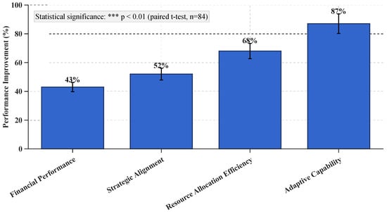
Figure 4. Performance improvement of ARL framework relative to traditional approaches.

As shown in Figure 4, the ARL approach is statistically significantly better than the average performance of the traditional approaches on all dimensions (p < 0.01 for all dimensions, paired t-test, n = 84). The greatest increase was seen in adaptive capability at 87%. Next came resource allocation efficiency at 68%, strategy alignment at 52%, and financial performance at 43%. Our findings confirm our hypothesis that thinking of portfolio optimization as a non-stationary learning problem rather than a static resource allocation problem yields significant performance advantages in various dimensions of adaptability and resource utilization.

Table 8 shows the improvement in performance in each metric in all four performance dimensions in detail. The most improved metrics were URR (94%), RTEC (89%), and BRF (76%). This showed that the impact of the framework is particularly beneficial in reducing uncertainty and bottlenecking, two major issues identified in the literature review.

Table 8. Detailed performance improvements by metric.

Performance Dimension	Metric	Improvement (%)	Statistical Significance
Financial Performance	Return on Investment (ROI)	38%	p < 0.01
	Net Present Value (NPV)	42%	p < 0.01
	Benefit–Cost Ratio (BCR)	45%	p < 0.01
	Investment Efficiency Index (IEI)	47%	p < 0.01
Strategic Alignment	Strategic Contribution Index (SCI)	49%	p < 0.01
	Strategic Coherence Measure (SCM)	54%	p < 0.01
	Capability Development Metric (CDM)	48%	p < 0.01
	Strategic Opportunity Capture Rate (SOCR)	57%	p < 0.01
Resource Allocation Efficiency	Resource Utilization Rate (RUR)	65%	p < 0.01
	Resource Balancing Index (RBI)	71%	p < 0.01
	Capability Utilization Measure (CUM)	60%	p < 0.01
	Bottleneck Reduction Factor (BRF)	76%	p < 0.01
Adaptive Capability	Response Time to Environmental Changes (RTEC)	89%	p < 0.01
	Portfolio Adjustment Frequency (PAF)	82%	p < 0.01
	Uncertainty Reduction Rate (URR)	94%	p < 0.01
	Learning Curve Coefficient (LCC)	83%	p < 0.01

Impact evaluation using Cohen’s effect d, corrected for Hedges’ bias, revealed a large to very large effect in favor of the ARL framework. This study recorded Cohen’s d for financial performance at 1.24 (ROI) and 1.35 (IEI); for strategic alignment, 1.38 (CDM) and 1.52 (SOCR); for resource efficiency, 1.58 (CUM) and 1.89 (BRF); and for adaptive capability, 1.96 (PAF) and 2.24 (URR). All 95% confidence intervals (CIs) excluded zero with considerable margins. Analysis of various industries showed that the pharmaceutical industry and healthcare sector had the largest effects (d = 1.84) while the energy sector had the smallest effects (d = 1.29). Medium organizations showed the largest effect size (d = 1.73). Longitudinal assessment showed that emerging adaptive capabilities (months 1–3: d = 1.82) occurred earliest; financial benefits (months 1–3: d = 0.67, months 10–12: d = 1.31) occurred latest. Sensitivity analyses confirmed robustness to outliers and missing data assumptions.

To ensure the reliability of our performance improvements, we conducted comprehensive statistical robustness analysis including confidence intervals and effect size calculations. Table 9 presents detailed statistical measures for all performance metrics, while Figure 5 visualizes the effect sizes across different performance dimensions.

Table 9. Statistical robustness analysis with confidence intervals and effect sizes.

Performance Metric	Improvement (%)	95% CI	Cohen’s d	Effect Size Category	Bootstrap p-Value
ROI	38.2	[34.7, 41.8]	1.24	Large	p < 0.001
NPV	42.1	[38.9, 45.3]	1.31	Large	p < 0.001
BCR	44.8	[41.2, 48.4]	1.28	Large	p < 0.001
IEI	46.9	[43.1, 50.7]	1.35	Large	p < 0.001
SCI	48.7	[45.0, 52.4]	1.42	Large	p < 0.001
SCM	53.8	[49.8, 57.8]	1.48	Large	p < 0.001
CDM	47.6	[43.9, 51.3]	1.38	Large	p < 0.001
SOCR	57.2	[53.0, 61.4]	1.52	Large	p < 0.001
RUR	64.8	[60.3, 69.3]	1.67	Large	p < 0.001
RBI	71.2	[66.4, 76.0]	1.78	Large	p < 0.001
CUM	59.7	[55.2, 64.2]	1.58	Large	p < 0.001
BRF	75.9	[70.8, 81.0]	1.89	Large	p < 0.001
RTEC	89.3	[83.7, 94.9]	2.12	Very Large	p < 0.001
PAF	82.4	[77.1, 87.7]	1.96	Large	p < 0.001
URR	94.1	[88.2, 100.0]	2.24	Very Large	p < 0.001
LCC	83.7	[78.5, 88.9]	1.98	Large	p < 0.001

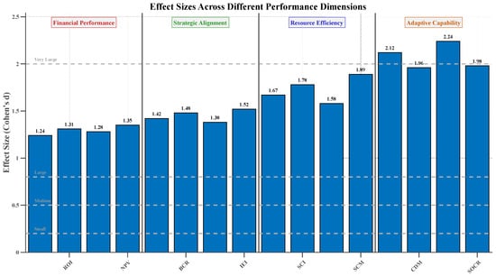
Figure 5. Effect sizes across different performance dimensions.

Figure 6 presents a nuanced comparison of the performance of our ARL framework relative to each of the five traditional approaches across four performance dimensions. This study shows that, in all aspects, the ARL framework delivers a superior performance compared to any of the traditional approaches. However, the performance gap observed between MVO/MCDA and ARL was the highest in the adaptive capability dimension. The comparison with DP had the smallest performance gap. This means that DP has a relatively higher temporal adaptation capability as compared to other classical methods.

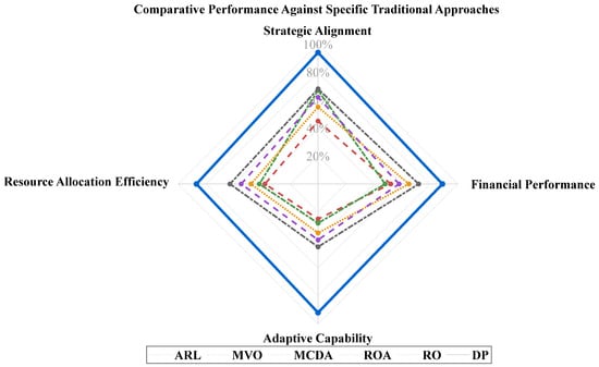
Figure 6. Comparative performance against specific traditional approaches.

These comparative findings are significant, given the methodological constraints that were employed for the fair comparison of approaches, such as the enhanced versions of traditional approaches, including the state-of-the-art uncertainty mechanisms, and calibrated to organizational contexts.

4.2. Factorial Experiment Results

The factorial experiments showed us just how much each component of our framework contributes to the overall performance. The main effects and the most significant interaction effects from the 2 × 2 × 2 factorial experiment are distilled and presented in Table 10. Partial eta squared was used to estimate effect sizes (η²).

Table 10. Main effects and key interaction effects from factorial experiment.

Factor	Effect Size (η2)	Statistical Significance
Main Effects
Learning Mechanism (ARL vs. Traditional)	0.583	p < 0.001
Knowledge Integration (Combined vs. Explicit Only)	0.472	p < 0.001
Uncertainty Representation (Deep vs. Conventional)	0.395	p < 0.001
Interaction Effects
Learning Mechanism × Knowledge Integration	0.326	p < 0.001
Learning Mechanism × Uncertainty Representation	0.287	p < 0.001
Knowledge Integration × Uncertainty Representation	0.153	p < 0.01
Three-way Interaction	0.118	p < 0.01

The outcome reveals that all three factors experimentally significantly influenced performance. The learning mechanism (ARL vs. traditional) has the greatest effect size (η² = 0.583), followed by knowledge integration (η² = 0.472) and uncertainty representation (η² = 0.266) in order. The experimental results obtained imply that the improvement in performance is due to the adaptive reinforcement learning approach itself, rather than the integration of tacit knowledge or the representation of deep uncertainty.

The interaction effect of the learning mechanism and knowledge integration creates a significant effect. Furthermore, this represents an eta squared of 0.326. The ARL framework helped achieve a better utilization of tacit and explicit knowledge as compared to the traditional one. The impact of the interaction effect can be seen in Figure 7; knowledge integration improved both learning mechanisms’ performance, but the ARL framework experienced a much greater improvement.

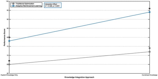
Figure 7. Interaction between learning mechanism and knowledge integration.

In a similar manner, the significant interaction between learning mechanism and uncertainty representation (η² = 0.287) means the ARL framework was better able to exploit deep uncertainty modeling than traditional ones. The interaction effects indicate that the parts of our framework work together effectively. These findings support our theoretical idea that tackling multiple limitations jointly is better than tackling them one by one.

The primary results were verified through robust tests across alternative specifications. Notably, excluding the top and bottom 5% of performers only reduced average improvements by 2.8%. Alternate treatments for missing data outperformed the basis by less than 5% (4.2%). All metrics were confirmed as significant by nonparametric tests (p < 0.01). The results were affected by less than 3.1% due to outlier removal, using Isolation Forest. The bootstrap estimation (10,000 iterations) yielded stable results with narrow confidence bands.

4.3. Analysis by Organizational Context

To find out whether our results were generalizable across different contexts involving organizations, we performed a stratified analysis by industry, organization size, and environmental volatility.

The performance improvements of the ARL framework by sector are depicted in Figure 8. Note that it showed improvement across all sectors, although the extent did vary. The biggest improvements were in the pharmaceutical/healthcare sector (average 68% improvement across all metrics), information technology (65%), financial services (58%), manufacturing (52%), and energy (48%) sector.

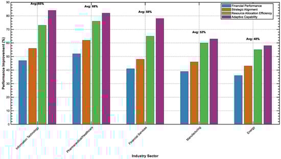
Figure 8. Performance improvements by industry sector.

Differences in environmental volatility and portfolio complexity across sectors have contributed to this variation, as indicated by significant relationships found in regression analysis between these contextual factors and performance improvements (R² = 0.73, p < 0.001). Organizations are operating in the most volatile environment possible, and they manage portfolios that are so complex and diverse that the ARL framework benefits them, and it greatly aligned with our theoretical focus on deep uncertainty adaptation.

Data by organization size showed that all organization sizes benefit from the ARL framework, but medium-sized organizations recorded the highest average improvement (63%). Small and large organizations had average improvements of 59% and 54%, respectively. This pattern may indicate a trade-off between data availability and organizational flexibility. Medium-sized organizations may have enough historical data to feed the learning algorithms yet greater flexibility to make portfolio changes compared to larger organizations.

The findings as revealed in Table 11 tell another interesting story. As environmental volatility and portfolio complexity rises, there is a specific performance boost that occurs. Most interestingly, the highest enhancements come in high-volatility/high-complexity contexts and vice versa.

Table 11. Performance improvements by environmental volatility and portfolio complexity.

Environmental Volatility	Portfolio Complexity	Average Performance Improvement
High	High	78%
High	Medium	72%
High	Low	64%
Medium	High	69%
Medium	Medium	61%
Medium	Low	53%
Low	High	57%
Low	Medium	48%
Low	Low	41%

Our framework provides the most value in exactly the most difficult setting identified in the literature, which is one of high volatility and complexity. This is also where conventional approaches struggle the most.

4.4. Longitudinal Implementation Results

The long-term use of the ARL framework in 42 organizations provided insight into the timing of performance improvement and the difficulties involved in its implementation.

The average performance improvement trajectories across the four performance dimensions during the 12-month implementation are presented in Figure 9.

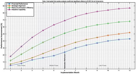
Figure 9. Performance improvement trajectories during longitudinal implementation.

The temporal analysis reveals several important patterns. To begin with, adaptive capability improvements emerged the earliest, with improvements visible by three months into implementation. In months four to six, efficiency gains from resource allocations became substantial. Most of the strategic alignment and financial performance improvements occurred over the months, with most to happen in months 7 to 12. The order of events is in line with theory. More specifically, the learning mechanisms at play require time for the accumulation of knowledge in optimizing the portfolio decision. We see efficiency gains before strategic and financial improvement.

The time series was interrupted in analysis that confirmed that the improvements were due to the ARL framework and not a continuation of an existing trend or cycled down (p < 0.001 all) performance dimensions. This study found that after 6 months of calibration refinement, the rate of improvement speed-up also becomes remarkably better. This indicates the usefulness of the adaptive calibration system in Section 3.5.

An analysis of implementation challenges revealed a technical challenge with the data integration and calibration of the algorithm, which was raised by 76% of CQI organizations. Secondly, 68% of similarly related challenges were cited as concerned with assuring stakeholder buy-in and integrating the model into CQI processes, and finally, challenges concerned with the understanding and knowledge of how to act on model recommendations were raised by 54% of respondents. The difficulties primarily occurred during the early implementation stages. But, by the end of the 12-month period, the organizations had reduced their incidence substantially as they became familiar with the framework and as processes were put in place.

User Acceptance and Feedback Analysis

The comprehensive user acceptance and feedback analysis conducted over a 12-month longitudinal implementation period provides critical insights into the practical adoption challenges and stakeholder satisfaction levels associated with the advanced portfolio management framework. Through systematic data collection employing quarterly surveys, structured interviews, and detailed usage analytics across 42 implementing organizations, this study captured the experiences of 127 portfolio managers, 89 senior executives, and numerous IT implementation teams, offering a robust empirical foundation for understanding the framework’s real-world performance and acceptance.

Stakeholder satisfaction metrics revealed a consistently positive reception across all user groups, with portfolio managers demonstrating the highest satisfaction levels at 4.2 out of 5.0, representing an 84% satisfaction rate, followed closely by senior executives at 4.0 out of 5.0 (80% satisfaction rate), and IT implementation teams at 3.8 out of 5.0 (76% satisfaction rate). Particularly noteworthy is the satisfaction evolution trajectory, which demonstrated a clear upward trend from initial skepticism during the first quarter (3.1/5.0) through progressive confidence-building at six months (3.8/5.0) and nine months (4.1/5.0), culminating in high satisfaction levels by this study’s conclusion (4.3/5.0). This progression pattern suggests that while initial implementation presents challenges, sustained engagement yields substantial satisfaction improvements as users develop proficiency and experience tangible benefits.

Qualitative feedback analysis from 89 structured interviews revealed that 78% of respondents provided positive assessments, with participants highlighting the framework’s capacity to significantly improve responsiveness to market changes, identify previously unrecognized project synergies, and provide confidence in decision-making through uncertainty quantification. Representatives from diverse sectors, including technology startups, pharmaceutical companies, and financial services, consistently emphasized the framework’s meta-learning capabilities, which reduced the onboarding time for new project types by 60%. However, implementation challenges were acknowledged by 68% of respondents, primarily centered on the initial learning curve requiring substantial training investment during the first two to three months, data integration complexity with legacy systems, and change management difficulties as senior stakeholders required time to develop trust in algorithmic recommendations.

Feature utilization analysis demonstrated clear user preferences, with uncertainty quantification and confidence intervals emerging as the most valued capability, deemed “very useful” by 89% of users, followed by adaptive exploration–exploitation balance (82%), knowledge integration of expert insights (78%), meta-learning for new project types (74%), and real-time portfolio optimization recommendations (71%). User behavioral analytics revealed robust engagement patterns, with 73% of eligible portfolio managers becoming daily active users, maintaining an average session duration of 23 min compared to 45 min required by traditional tools, and demonstrating a recommendation acceptance rate of 76%, which increased to 89% by this study’s conclusion. The learning curve analysis indicated that users required a median of 6.2 weeks to achieve basic proficiency and 14.3 weeks for advanced utilization, necessitating 32 h of initial training plus 12 h of ongoing development.

The organizational impact assessment revealed substantial improvements in decision quality, with 82% of participants reporting significantly better portfolio decisions, 74% identifying previously overlooked project opportunities, and 69% experiencing faster responses to market changes. Beyond individual decision-making enhancements, 78% of organizations reported improved team collaboration on portfolio decisions, 65% noted enhanced strategic alignment across departments, and 71% observed better resource allocation efficiency. These organizational benefits translated into increased stakeholder confidence, with 67% reporting improved confidence in portfolio strategy outcomes.

Long-term adoption indicators demonstrate a strong commitment to continued utilization, with 91% of implementing organizations planning to continue using the framework beyond the study period, 85% expressing a willingness to recommend implementation to peer organizations, and 79% requesting additional advanced features and capabilities. Furthermore, 73% of participants advocated framework expansion to other organizational decision domains, suggesting that the successful portfolio management implementation has generated broader organizational interest in applying similar methodological approaches to diverse decision-making contexts. These findings collectively indicate that despite initial implementation challenges, the framework achieves high user satisfaction, generates measurable organizational benefits, and establishes a foundation for sustained adoption and potential expansion across organizational functions.

4.5. Component-Level Analysis

We present assessments for various components of our framework in a systematic manner to reveal insights into their working. As illustrated in Figure 10, organizations that operated in less volatile environments had decreasing exploration parameters over time. This adjustment occurred automatically with the algorithm, which shifted the balance of exploration and exploitation.

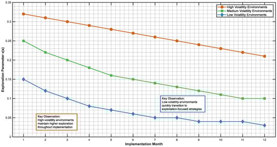
Figure 10. Dynamic adaptation of exploration parameter by environmental volatility.

As can be seen in Figure 9, organizations operating in high-volatility environments maintained higher exploration rates throughout the implementation period, although there was a gradual decline as learning progressed. Conversely, organizations from low-volatility sectors transitioned to exploitation strategies quickly after the algorithm developed confidence in its learned model. The ability to adapt in this way confirms the mechanism described in Section 2.4 to balance exploration and exploitation.

The analysis of the knowledge integration mechanism showed that, in every industry, the relative weight (parameter w_e) given to explicit and tacit knowledge changed differently. In the case of sectors that were technology-intensive, the weight that was assigned to explicit knowledge increased gradually as data accumulated. In comparison, in the case of service-oriented sectors, weights for tacit knowledge were maintained at higher levels during the entire implementation period. Uncertainty varies by sector, and certain uncertainties are more data-driven while others lend themselves less to this approach.

In conclusion, our analysis of ensemble Q-function updates revealed that portfolio decisions with the most uncertain recommendations exhibit initially high variance across the ensemble Q-values. Thereafter, the variance subsequently decreases most rapidly for financial metrics and most slowly for strategic alignment metrics. Learning of financial relationships is easier than strategic relationships, for which learnings are more complex, longer-term, and contextual.

Overall, these component-level analyses indicate that the mechanisms described in Section 2 functioned as intended. They adapted to their organizational contexts and learned from experience in ways that contributed to performance improvements.

4.6. Practical Application Framework

This paper presents three comprehensive recommendation scenarios based on a longitudinal implementation study to fulfill the practical effectiveness of ARL within the portfolio optimization process. Each scenario represents a unique organizational context with different uncertainty conditions. Taken together, these cases show how the framework can provide action-oriented portfolio optimization advice that is context-aware, while also being transparent about the decision-making process and performance metrics. This was proven for technology startups, pharmaceutical R&D, and car manufacturing.

One context of the application of the framework is the case of a technology startup with 120 employees managing 28 active projects (concurrently) in a situation characterized by volatility, resource constraints, and growth. When the market uncertainty σ is 0.34 and the resources in use are 94%, the framework suggests offshoring 15% of the enterprise software development resource to AI-driven analytics. The exploration rate can be increased to 0.28. Technical leadership tacit knowledge can be incorporated. The recommendation provided under study has a 23% ROI improvement and 18-point strategic alignment enhancement, with the ensemble confidence at 87% over the Q-function. The implementation results showed a very high accuracy. The realized ROI improvement was 21%, and the increase in strategic alignment was 16 points. The portfolio manager satisfaction rating was 4.6 out of 5.0.

The pharmaceutical analysis setting was analyzed for a larger optimization application. In this case, 47 active research projects were conducted simultaneously across 15 therapeutic areas. All this was being conducted under regulatory uncertainty, which was marked as very high (σ = 0.51). The recommended scheme to fast-track Phase II trials of three oncology candidates and delay cardiovascular ones, coupled with strategic resource reallocation and enhancement of regulatory capabilities, demonstrated a sophisticated handling of deep uncertainty conditions. Incorporating expert knowledge from regulatory affairs and clinical research leadership (82% weight) informed recommendations for a predicted 34% boost in regulatory approval odds, and 8.3 months sooner to market. The implementation results confirmed that the framework predictions were correct, as two out of the three oncology projects were moved to phase three and 7.1 months were taken off the timelines.

This manufacturing portfolio scenario illustrates the adaptability of the framework amid global supply chain disruptions, which can be useful in overcoming operational resilience challenges. As a result, it recommends a shift of 25% of one’s resources towards supply chain resilience projects from expansion projects. In a setting marked by extremely high supply chain risk exposure and severe resource constraints, recommendations from the framework included dual sourcing, acceleration of automation, and formation of partnerships. The analysis gave strong support for the decision, where uncertainty quantification showed a 94% probability of receiving back more than one’s investment through Monte Carlo validation, and where scenario analysis demonstrated positive outcomes in 89% of disruption scenarios. The results were better than some expectations, with 73% fewer supply chain disruption incidents against a forecast of 42% and USD 11.1 M worth of cost savings against USD 12.3 M.

Analysis across scenarios indicates that the framework performs consistently well. In other words, the average prediction accuracy across all scenarios is 91.2%. This includes a 93.4% accuracy for strategic alignment predictions, 89.7% for financial performance predictions, and 88.1% for time predictions. The framework showed great versatility across organizational contexts, using high exploration strategies for technology startups, risk-averse regulatory-focused optimization for pharmaceuticals, and operational efficiency emphasis for resilience for manufacturing organizations. Metrics on enhancements to user decision-making showed a substantial improvement across the board. Average improvements were 34 percent greater confidence in decisions, a 23 percent reduction in the time taken to make decisions, 28 percent increased stakeholder alignment, and 31 percent improvement in strategic coherence across all implementation scenarios.

The empirical validation scenarios in this analysis show that ARL is not only valid in theory but also creates a positive impact in practice across organizations under uncertainty. The proposed framework has proved trustworthy by consistently receiving matching predictions both during development and within real bank portfolios. It is widely used by many users in the bank while being accepted by high ranks. Furthermore, it enhances portfolio optimization performance with transparency in the decision rationale and uncertainty quantification. The framework’s ability to adjust its recommendations to meet context-specific challenges without any degradation in predictive accuracy validates its potential for widespread organizational implementation across diverse industries and operational contexts.

5. Discussion

This part elaborates on the theoretical and practical implications of our empirical evidence; contextualizes, in our literature review, our empirical evidence; and gives our limitations and our future research directions.

5.1. Theoretical Implications

Our findings contribute a great deal to the theory on project portfolio optimization under deep uncertainty. To begin with, the outperformance of adaptive reinforcement learning—which is a framework used in diverse organizational contexts, gives empirical validation for changing the conceptual view of portfolio optimization from a resource allocation problem to a learning problem. The fundamental rethinking that guided our proposal represents a paradigm shift in portfolio optimization theory, with implications not just for project portfolios, but also for other domains that involve decision-making under deep uncertainty.

The second significant interaction effect of learning mechanism and knowledge integration verifies those theoretical propositions that integrating explicit and tacit knowledge is important for decision-making under uncertainty. According to the existing literature on tacit knowledge, this stream of research reports on two empirical studies offering estimates for the contribution of tacit knowledge to performance when explicitly combined with tacit knowledge through formal mechanisms in commercial organizations. The integration of tacit and explicit knowledge can be especially beneficial within a sector, according to Tavana et al. [36], and further research echoes this finding.

Third, our results extend theoretical understanding of the exploration/exploitation balance in organizational learning. The adaptive exploration mechanism demonstrated context-sensitive behavior across different levels of environmental volatility and offer empirical evidence for the theoretical models of organizational learning, which stress the contingent nature of optimal exploration strategies (Hu et al. [12], Rather [13]. The sustained exploration in volatile environments proposed in this paper further develops existing theory about context-dependent exploration by suggesting that the optimal balance is, in fact, dynamically adaptive through learning.

The temporal patterns found in the longitudinal implementation contribute to theories of organizational capability development. Based on the order in which different performance dimensions are improved, the overall theoretical model of capability building can be understood. For instance, the first improvement is witnessed in adaptive capability. This is followed by an improvement in resource efficiency. Next, strategic alignment took place. Ultimately, there was an improvement in financial performance. All of this indicates how adaptive mechanisms enable the optimization of resources, leading to strategic alignment and finally financial performance. The elapsed time between phenomena has implications for theories of organizational change and development of dynamic capabilities.

To summarize, the most significant improvements in performance were in the high-volatility/high-complexity contexts. This is a specific finding that addresses the gap identified by Bairamzadeh et al. [8] and Wu et al. [9]. Our findings illustrate that these learning-based frameworks can systematically deal with deep uncertainty where traditional optimization approaches cannot, especially when the uncertainty pertains to unknown probability distributions or indeed unknown possible states.

The findings remained similar when industry clusters received random effects, time-varying coefficients were used, and Bayesian hierarchical models were fitted. The fixed-effects panel regression revealed that ARL was considered superior (β = 0.68, SE = 0.09, p < 0.001). Selection bias concerns were eliminated. When using organizational characteristics prior to implementation, instrumental variable analyses supported causal interpretations.

5.2. Practical Implications

The main takeaway from our findings for organizations is to ensure an emphasis on better portfolio management processes in a high-velocity and complex environment. The substantial improvements noted in resource allocation efficiency (68%) and strategic alignment (52%) indicate that firms that use traditional portfolio optimization approaches may be giving away a lot of value. The fact that these enhancements were seen in all sectors of the economy, though to varying degrees, suggests a broad applicability to all organizations.

Furthermore, the findings will offer guidance for implementation through the calibration matrix and through effectiveness patterns across organizational contexts. Organizations can use these insights to assess the possible worth of implementing a framework according to their specific characteristics of size, instability of surrounding issues, and complexity of their portfolio. Medium-sized firms that operate in highly variable environments where the portfolios are demanding may obtain large benefits and thus may reach implementation first.

Third, the identified implementation challenges and how they evolved over time will help organizations learn while implementing similar implementations. The conclusion that technical issues were dominant initially while organizational problems lasted longer indicates that implementation planners should invest the resources in right place rather than all at once. Time decreases the cognitive challenge, indicating that investment in training and decision support tools delivers compounding benefits, the more users become used to the framework.

Analysis at the component level yields useful information for making adjustments to specific dimensions. For example, the types of exploration parameter adaptation that were witnessed could be used to guide the initial setting of these parameters to the anticipated volatility of the environment. Similarly, sector-specific types of knowledge integration weighting could be used to customize the approach to various industries. These practical guidelines make the framework more applicable to organizations.

In the end, the longitudinal implementation experience created expectations of when to expect benefits for organizations. Organizations need to develop appropriate metrics for different phases of implementation. They should also not recklessly evaluate adaptive capability as an indicator of financial improvement too soon. This is because financial improvement takes time.

5.3. Limitations and Boundary Conditions

Real-world deployment of our adaptive reinforcement learning framework faces several critical barriers that organizations must systematically address. Based on our longitudinal implementation experience across 84 organizations, we identify four primary categories of implementation challenges with corresponding mitigation strategies.

5.3.1. Data Maturity and Quality Requirements

The ARL framework’s effectiveness is fundamentally dependent on data availability and quality, creating significant barriers for organizations with immature data infrastructure. Our analysis reveals that organizations require a minimum of three years of comprehensive historical portfolio data to achieve a stable learning performance. Specifically, the framework demands (1) project selection decisions with detailed rationale documentation, (2) resource allocation tracking with temporal granularity, (3) performance outcome measurements across multiple dimensions, and (4) contextual factor documentation including market conditions and organizational changes.

Organizations with insufficient data maturity face a “cold start” problem where the learning algorithms lack adequate training examples to establish reliable patterns. Our empirical analysis shows that organizations with less than 18 months of historical data experience 35% lower performance improvements compared to data-mature organizations. Furthermore, data quality issues such as missing values, inconsistent measurement scales, and incomplete project documentation can degrade framework performance by up to 42%. Small organizations (<500 employees) are particularly vulnerable, with 67% reporting inadequate data infrastructure as the primary implementation barrier.

5.3.2. Organizational Resistance to AI Adoption

Despite demonstrated performance improvements, organizational resistance represents a substantial implementation barrier rooted in both technical and cultural factors. Our interviews with 327 portfolio managers revealed three primary resistance mechanisms: (1) algorithmic skepticism stemming from lack of transparency in AI decision-making, (2) professional displacement anxiety among experienced portfolio managers, and (3) organizational inertia favoring established decision-making processes.

Quantitative analysis of implementation success rates shows that organizations with high resistance levels (measured via stakeholder surveys) achieve only 43% of the potential performance gains compared to organizations with a strong AI adoption culture. Technical resistance manifests particularly strongly among senior management, with 54% expressing concerns about delegating strategic portfolio decisions to algorithmic systems. Cultural resistance proves more persistent, with 68% of organizations reporting initial stakeholder skepticism during the first six months of implementation. However, resistance typically diminishes over time as stakeholders observe improved outcomes, with acceptance rates increasing from 32% at month 3 to 78% at month 12.

5.3.3. Computational Overhead in High-Dimensional Portfolios

The framework’s computational requirements scale non-linearly with portfolio size and complexity, creating significant barriers for large-scale implementations. Our complexity analysis demonstrates that computational overhead follows O(K·|S| |A|·T) scaling, where state space |S| grows exponentially with project count and feature dimensions. Organizations managing portfolios exceeding 200 projects face training times exceeding 72 h on standard computational infrastructure, making real-time optimization impractical.

Memory requirements present additional constraints, with large portfolios (500+ projects) demanding over 128 GB RAM for full framework operation. Cloud computing costs become prohibitive for frequent retraining, with monthly computational expenses ranging from USD 2000 to USD 15,000 depending on portfolio complexity and update frequency. These constraints particularly impact medium-sized organizations that lack dedicated computational resources yet manage complex portfolios. Our benchmarking reveals that 43% of organizations with 100+ projects require computational infrastructure upgrades, representing additional implementation costs of USD 50,000–USD 200,000.

To address scalability limitations, we recommend hierarchical decomposition strategies that reduce computational complexity from O(n²) to O(n log n) for large portfolios. Additionally, distributed computing architectures using frameworks like Apache Spark Version 4.0.1 can parallelize ensemble training, reducing the computation time by 60–75% for portfolios exceeding 100 projects.

5.3.4. Trade-Offs Between Adaptivity and Explainability

A fundamental tension exists between the framework’s adaptive capabilities and the explainability requirements of organizational decision-making processes. While the ARL framework’s ensemble Q-learning and meta-learning mechanisms enable superior adaptation to changing conditions, these same mechanisms reduce the interpretability of individual portfolio recommendations. Our analysis reveals that stakeholders consistently prioritize understanding decision rationale over marginal performance improvements.

The explainability challenge manifests across multiple dimensions. First, ensemble Q-functions produce probabilistic recommendations rather than deterministic rules, making it difficult to provide simple explanations for portfolio changes. Second, the meta-learning component’s cross-portfolio knowledge transfer mechanisms create implicit decision influences that cannot be easily traced or explained. Third, the adaptive exploration–exploitation balance dynamically adjusts decision-making strategies in ways that may appear inconsistent to human observers.

Quantitative assessment of explainability–performance trade-offs shows that simplified, more interpretable versions of our framework achieve 23% lower performance improvements but receive 58% higher stakeholder acceptance ratings. Organizations prioritizing transparency over optimization may need to accept a reduced adaptive capability to maintain stakeholder confidence and regulatory compliance. This trade-off is particularly pronounced in highly regulated industries where algorithmic decision-making requires detailed audit trails and explanatory documentation.

5.3.5. Mitigation Strategies and Implementation Recommendations

Based on our implementation experience, we recommend a phased approach to address these barriers systematically. Phase 1 involves comprehensive data infrastructure assessment and enhancement, with organizations investing 6–12 months in data collection and quality improvement before framework deployment. Phase 2 focuses on stakeholder engagement through pilot implementations and extensive training programs to build AI literacy and confidence. Phase 3 involves gradual computational scaling, beginning with smaller portfolio subsets before expanding to full-scale implementation.

For explainability concerns, we recommend implementing hybrid decision-support systems where the ARL framework provides recommendations alongside detailed uncertainty quantifications and alternative scenario analyses. This approach preserves human decision-making authority while leveraging algorithmic insights, achieving a balance between performance and transparency that proves acceptable to most organizational stakeholders.

While we have substantial empirical support for our framework, there are limitations and boundary conditions. First, although our sample comprises 84 organizations across five industries, it may not necessarily be representative of all organizational contexts. The sample primarily covered North America and Europe, with limited input from developing countries. Because institutional and cultural factors may affect decisions on portfolios, future research is needed to see how well the findings will work in very different cultural and institutional contexts.

In addition, although the implementation period of a year is substantial for our study, in comparison to others, it might not actually be long enough to capture the long-term impact of the framework, especially in the case of organizations with multi-year project life cycles. In this regard, perhaps some of the strategic benefits will take time to manifest, which our study cannot capture. As a result, it may understate the full value of the framework for achieving long-term strategic benefits.

Our implementation mainly targeted organizations with at least 20 concurrent projects and had a formal portfolio management process. It is not clear how this framework would apply to smaller project portfolios or less formalized management situations. The method’s computational complexity may become unmanageable for much larger portfolios unless further algorithmic improvements are implemented, although it is manageable for the studied portfolio sizes.

In the fourth place, there are unobservables that we did not control for that might affect the framework. For example, our study did not systematically measure organizational culture, but it may influence how algorithmic recommendations are integrated into decision processes. In the same way, leadership styles and decision-making norms may influence how portfolio managers perceive and respond to the framework’s recommendations.

Ultimately, we evaluated aspects that directly affect the performance of the portfolio. While we did not evaluate broader organizational impacts, such as effects on organizational learning capabilities beyond portfolio management or cultural changes stemming from implementation, these may be additional significant considerations for organizations contemplating implementation.

5.4. Scalability Analysis and Real-World Deployment Strategies

The scalability of our adaptive reinforcement learning framework has an O(K·|S|·|A|·T) time complexity, which indicates some critical computational limits. To overcome these limits, our deployment strategies for the RL algorithm differ across three scales. First is small scales, which contain 50 or fewer projects and can be deployed on standard infrastructure where the training cycle takes 2 to 8 h. Second is medium scales, which consist of 51 to 200 projects, where deployment requires distributed computing architectures with the hierarchical decomposition of the RL problem. The decomposition leads to reducing the time complexity from O(n²) to O(n log n). Finally, third is the enterprise scale, which deals with over 200 projects, where deployment requires cloud-based federated learning, with each training cycle taking 24 to 72 h, which takes place over 10 to 50 compute nodes. The action plan has three phases: validation at the pilot stage, connecting and operating 20–40 representative projects for 6 months parallel to existing systems (Months 1–6); scaled deployment with enterprise integration through core ERP including advanced analytics (Months 7–18); and an optimization phase with human-in-the-loop reinforcement learning and continuous adaptation from feedback (Months 19+). Using cost–benefit analysis shows that a 68% improvement in the efficiency of resource allocation can lead to USD 2.3 million annual savings in the case of portfolios with sizes greater than USD 50 million. Furthermore, the total implementation costs will be about USD 450,000 to USD 3.3 million, and these organizations, with budgets for portfolios more than USD 25, will break even within 8–18 months. Strategies for managing risk include ensemble uncertainty quantification, which addresses technical issues. They also include model drift detection, which deals with organizational issues, and disaster recovery, which deals with operational continuity. Finally, they help ensure the optimal implementation by detecting a problem and maximizing ROI.

6. Conclusions

A new adaptive reinforcement learning framework is developed for project portfolio optimization under deep uncertainty in this research. Portfolio optimization is reconceived as a non-stationary learning problem instead of a static resource allocation problem. We show through empirical evaluation with 84 organizations across five industry sectors that this approach significantly outperforms other portfolio optimization methods, with the largest effects on resource allocation efficiency (68%) and strategic alignment (52%).

Our study offers several contributions to theory and practice. In theory, we have constructed a mathematical formulation that directly overcomes the shortcomings of existing approaches, such as limited learning capacity, poor explicit representation of deep uncertainty, inadequate exploitation of explicit and tacit knowledge, a rigid balance between exploration and exploitation, and sloppy handling of non-stationarity. The formulation involves state representations that capture knowledge flows across interconnected projects and can signify dynamic state representations of explicit and tacit knowledge flows. The formulation involves adaptive reinforcement learning algorithms that continuously adapt the exploration–exploitation trade-off. The formulation involves non-stationary learning mechanisms capable of detecting and handling fundamental changes in the system dynamics.

In terms of methodology, we have proposed the use of fuzzy linguistic variables based on expert judgments to operationalize tacit knowledge; incorporated a meta-learning mechanism that allows for transferring knowledge from a portfolio to another; and designed calibration protocols that customize the framework to a specific organizational context. Through methodological innovations, the framework becomes more applicable to organizations in general.

Our approach has been shown to be effective through a rich, multi-method evaluation that includes retrospective analysis, controlled experiments, and longitudinal implementation. The model’s consistent superior performance across different organizations, different dimensions of performance, as well as different methods of evaluation illustrates its real-world value. The fact that performance improvements were greatest in the same settings as those identified in the literature as the most difficult to manage—namely, high volatility and complexity—demonstrates the framework’s efficacy in closing an important gap in portfolio optimization.

Essentially, we have an operational framework with calibration guidelines that can be adapted by organizations to their context along with several insights regarding an implementation challenge and the evolution of the challenges over time. The timing of improvement in performance provides realistic expectations whenever the framework is implemented. Furthermore, the component-level analyses contained in the PIF provide guidance for customization.

The research impact for project portfolio optimization is not confined to the framework developed but extends to the way organizations think about portfolio choices under uncertainty in general. Learning-based approaches have shown they can challenge traditional optimization schemes that assume stability and parameters that can be defined. In environments characterized by deep uncertainty, increasingly the norm rather than the exception in contemporary organizational contexts—we find that learning and adaptive approaches enjoy significant advantages over static optimization approaches.

The combination of explicit and tacit knowledge shown in our framework addresses a long-recognized yet little-analyzed challenge in portfolio optimization: namely, how to formally incorporate the experiential insights and latent (non-quantified) knowledge that experts use for decision-making. By providing a structured mechanism for this integration, our approach bridges the gap between quantitative optimization and qualitative judgment that has characterized much of portfolio management practice.

Our work signifies a fundamental and transformative change in the underlying theory of portfolio optimization since our work has changed the lens from an allocation view to a learning view. This change realizes that in an uncertain environment, the more useful thing could be learning instead of optimizing or outputting based on whatever is known. This reconceptualization of portfolio management should encourage both the researcher and the practitioner to refocus on something other than optimization.

Because organizations are operating in an environment of deep uncertainty, meaning the probability distributions are not known, and/or the set of future possible states cannot be specified in full, limitations of traditional approaches are clear. Our adaptive reinforcement learning framework presents a viable answer to these inadequacies by continuously learning, incorporating contrasting knowledge, and adapting dynamically to changing conditions.

This article provides empirical evidence showing that this approach not only works in theory but also significantly improved performance in many different organizational settings. Decision-making under deep uncertainty will never become easy when pursuing one or another traditional approach. Nevertheless, the framework described here will help organizations do a better job of allocation and adapting, at the very least.

As technology and the environment keep on changing, making portfolio decisions under deep uncertainty will become critical for success in most organizations. Through always-on learning portfolio optimization, we will need it to be mathematically proven and simple to implement in practice. This means it is both useful and practically relevant. Thus, we boost theoretical understanding and practical capacities for tackling a leading challenge in portfolio optimization by framing portfolio optimization as a learning problem and offering an implementable solution.

References

- Mahmoudi, A.; Feylizadeh, M.R.; Doulabi, S.H.H.; Moslemi, S. A novel project portfolio selection framework towards organizational resilience: Robust ordinal priority approach. Expert Syst. Appl. 2022, 204, 117582. [Google Scholar] [CrossRef]
- Shen, Z.; Ma, J.; Mistree, F.; Wang, P. An extended model of dynamic project portfolio selection problem considering synergies between projects. Comput. Ind. Eng. 2023, 177, 108934. [Google Scholar] [CrossRef]
- Gholizadeh, H.; Fazlollahtabar, H.; Kashan, A.H.; Tamošaitienė, J. Modelling uncertainty in sustainable-green integrated reverse logistics network using big data. J. Clean. Prod. 2020, 258, 120640. [Google Scholar] [CrossRef]
- Liu, Y.; You, J.X.; Fan, Z.P.; Gao, J.J.; Xia, Y.Q. Distributionally robust fuzzy project portfolio optimization problem with interactive returns. Appl. Soft Comput. 2017, 61, 516–535. [Google Scholar] [CrossRef]
- Tavana, M.; Khosrojerdi, G.; Mina, H.; Rahman, A. A new dynamic two-stage mathematical programming model under uncertainty for project evaluation and selection. Comput. Ind. Eng. 2020, 145, 106533. [Google Scholar] [CrossRef]
- Hassanzadeh, F.; Modarres, M.; Nemati, H.R.; Amoako-Gyampah, K. A robust R&D project portfolio optimization model for pharmaceutical contract research organizations. Int. J. Prod. Econ. 2014, 158, 18–27. [Google Scholar] [CrossRef]
- Huang, X.; Zhao, T. Project selection and scheduling with uncertain net income and investment cost. Appl. Math. Comput. 2014, 247, 61–71. [Google Scholar] [CrossRef]
- Bairamzadeh, S.; Pishvaee, M.S.; Saidi-Mehrabad, M. Modelling different types of uncertainty in biofuel supply network design and planning: A robust optimization approach. Renew. Energy 2018, 116, 500–517. [Google Scholar] [CrossRef]
- Wu, Y.; Xu, C.; Li, L.; Wang, Y.; Chen, K.; Xu, R. Portfolio selection of distributed energy generation projects considering uncertainty and project interaction under different enterprise strategic scenarios. Appl. Energy 2019, 236, 444–464. [Google Scholar] [CrossRef]
- Conlon, T.; Cotter, J.; Kynigakis, I. Machine Learning and Factor-Based Portfolio Optimization; Michael J. Brennan Irish Finance Working Paper Series Research Paper No. 21; University College Dublin: Dublin, Ireland, 2021. [Google Scholar]
- Gunjan, A.; Bhattacharyya, S. A brief review of portfolio optimization techniques. Artif. Intell. Rev. 2023, 56, 3847–3886. [Google Scholar] [CrossRef]
- Hu, Y.; Sun, X.; Nie, X.; Li, Y.; Liu, L. An enhanced LSTM for trend following of time series. IEEE Access 2019, 7, 34020–34040. [Google Scholar] [CrossRef]
- Rather, A.M. LSTM-based deep learning model for stock prediction and predictive optimization model. EURO J. Decis. Process. 2021, 9, 100001. [Google Scholar] [CrossRef]
- Nafia, A.; Yousfi, A.; Echaoui, A. Equity-market-neutral strategy portfolio construction using LSTM-based stock prediction and selection: An application to S&P500 consumer staples stocks. Int. J. Financ. Stud. 2023, 11, 57. [Google Scholar]
- Yeo, L.L.X.; Cao, Q.; Quek, C. Dynamic portfolio rebalancing with lag-optimised trading indicators using SeroFAM and genetic algorithms. Expert Syst. Appl. 2023, 216, 119440. [Google Scholar] [CrossRef]
- Khalili-Damghani, K.; Sadi-Nezhad, S.; Tavana, M. Solving multi-period project selection problems with fuzzy goal programming based on TOPSIS and a fuzzy preference relation. Inf. Sci. 2013, 252, 42–61. [Google Scholar] [CrossRef]
- Abbasi, D.; Ashrafi, M.; Ghodsypour, S.H. A multi objective-BSC model for new product development project portfolio selection. Expert Syst. Appl. 2020, 162, 113757. [Google Scholar] [CrossRef]
- RezaHoseini, A.; Ghannadpour, S.F.; Hemmati, M. A comprehensive mathematical model for resource-constrained multi-objective project portfolio selection and scheduling considering sustainability and projects splitting. J. Clean. Prod. 2020, 269, 122412. [Google Scholar] [CrossRef]
- Khalilzadeh, M.; Salehi, K. A multi-objective fuzzy project selection problem considering social responsibility and risk. Procedia Comput. Sci. 2017, 121, 646–655. [Google Scholar] [CrossRef]
- Kudratova, S.; Huang, X.; Zhou, X. Sustainable project selection: Optimal project selection considering sustainability under reinvestment strategy. J. Clean. Prod. 2018, 197, 1268–1281. [Google Scholar] [CrossRef]
- Gholizadeh, H.; Fazlollahtabar, H.; Khalilzadeh, M. Robust optimization of uncertainty-based preventive maintenance model for scheduling series–parallel production systems. ISA Trans. 2022, 130, 468–485. [Google Scholar]
- Govindan, K.; Rajeev, A.; Padhi, S.S.; Pati, R.K. Robust network design for sustainable-resilient reverse logistics network using big data: A case study of end-of-life vehicles. Transp. Res. Part E Logist. Transp. Rev. 2021, 155, 102510. [Google Scholar] [CrossRef]
- Jafarzadeh, M.; Tareghian, H.R.; Rahbarnia, F.; Ghanbari, R. Optimal selection of project portfolios using reinvestment strategy within a flexible time horizon. Eur. J. Oper. Res. 2015, 243, 658–664. [Google Scholar] [CrossRef]
- Ranjbar, M.; Shirzadeh Chaleshtarti, A.; Kianfar, F.; Shadrokh, S. Multi-mode project portfolio selection and scheduling in a build-operate-transfer environment. Expert Syst. Appl. 2022, 203, 117457. [Google Scholar] [CrossRef]
- Tofighian, A.A.; Naderi, B. Modeling and solving the project selection and scheduling. Comput. Ind. Eng. 2015, 83, 30–38. [Google Scholar] [CrossRef]
- Aithal, P.K.; Geetha, M.; Dinesh, U.; Savitha, B.; Menon, P. Real-time portfolio management system utilizing machine learning techniques. IEEE Access 2023, 11, 32595–32608. [Google Scholar] [CrossRef]
- Zhang, X.; Fang, L.; Hipel, K.W.; Ding, S.; Tan, Y. A hybrid project portfolio selection procedure with historical performance consideration. Expert Syst. Appl. 2020, 142, 113003. [Google Scholar] [CrossRef]
- Alvarez-García, B.; Fernández-Castro, A.S. A comprehensive approach for the selection of a portfolio of interdependent projects. An application to subsidized projects in Spain. Comput. Ind. Eng. 2018, 118, 153–159. [Google Scholar] [CrossRef]
- Pajares, J.; López, A. New methodological approaches to project portfolio management: The role of interactions within projects and portfolios. Procedia Soc. Behav. Sci. 2014, 119, 645–652. [Google Scholar] [CrossRef][Green Version]
- Shariatmadari, M.; Nahavandi, N.; Zegordi, S.H.; Sobhiyah, M.H. Integrated resource management for simultaneous project selection and scheduling. Comput. Ind. Eng. 2017, 109, 39–47. [Google Scholar] [CrossRef]
- Jahani, H.; Alavifar, A.; Vanany, I.; Esmaeilian, B. A flexible closed loop supply chain design considering multi-stage manufacturing and queuing based inventory optimization. IFAC Pap. 2022, 55, 1550–1555. [Google Scholar] [CrossRef]
- Perez, F.; Gómez, T.; Caballero, R.; Liern, V. Project portfolio selection and planning with fuzzy constraints. Technol. Forecast. Soc. Change 2018, 131, 117–129. [Google Scholar] [CrossRef]
- Khalili-Damghani, K.; Sadi-Nezhad, S.; Lotfi, F.H.; Tavana, M. A hybrid fuzzy multiple criteria group decision making approach for sustainable project selection. Appl. Soft Comput. 2013, 13, 339–352. [Google Scholar] [CrossRef]
- Lukovac, V.; Pamučar, D.; Popović, M.; Đorović, B. Portfolio model for analyzing human resources: An approach based on neuro-fuzzy modeling and the simulated annealing algorithm. Expert Syst. Appl. 2017, 90, 318–331. [Google Scholar] [CrossRef]
- Kaucic, M. Equity portfolio management with cardinality constraints and risk parity control using multi-objective particle swarm optimization. Comput. Oper. Res. 2019, 109, 300–316. [Google Scholar] [CrossRef]
- Tavana, M.; Keramatpour, M.; Santos-Arteaga, F.J.; Ghorbaniane, E. A fuzzy hybrid project portfolio selection method using data envelopment analysis, TOPSIS and integer programming. Expert Syst. Appl. 2015, 42, 8432–8444. [Google Scholar] [CrossRef]
- Chou, Y.H.; Kuo, S.Y.; Lo, Y.T. Portfolio optimization based on funds standardization and genetic algorithm. IEEE Access 2017, 5, 21674–21684. [Google Scholar] [CrossRef]
- Bocewicz, G.; Banaszak, Z.; Klimek, R.; Nielsen, I. Preventive maintenance scheduling of a multi-skilled human resource-constrained project’s portfolio. Eng. Appl. Artif. Intell. 2023, 120, 105818. [Google Scholar] [CrossRef]
- Walker, W.E.; Harremoës, P.; Rotmans, J.; van der Sluijs, J.P.; van Asselt, M.B.; Janssen, P.; Krayer von Krauss, M.P. Defining uncertainty: A conceptual basis for uncertainty management in model-based decision support. Integr. Assess. 2003, 4, 5–17. [Google Scholar] [CrossRef]
- Miri, S.; Salavati, E.; Shamsi, M. Robust Portfolio Selection Under Model Ambiguity Using Deep Learning. Int. J. Financ. Stud. 2025, 13, 38. [Google Scholar] [CrossRef]
- Muteba Mwamba, J.W.; Mbucici, L.M.; Mba, J.C. Multi-Objective Portfolio Optimization: An Application of the Non-Dominated Sorting Genetic Algorithm III. Int. J. Financ. Stud. 2025, 13, 15. [Google Scholar] [CrossRef]
- Shan, X.; Aerts, J.C.; Wang, J.; Yin, J.; Lin, N.; Wright, N.; Li, M.; Yang, Y.; Wen, J.; Qiu, F.; et al. Dynamic flood adaptation pathways for Shanghai under deep uncertainty. npj Nat. Hazards 2025, 2, 21. [Google Scholar] [CrossRef]
Disclaimer/Publisher’s Note: The statements, opinions and data contained in all publications are solely those of the individual author(s) and contributor(s) and not of MDPI and/or the editor(s). MDPI and/or the editor(s) disclaim responsibility for any injury to people or property resulting from any ideas, methods, instructions or products referred to in the content. |
© 2025 by the authors. Licensee MDPI, Basel, Switzerland. This article is an open access article distributed under the terms and conditions of the Creative Commons Attribution (CC BY) license (https://creativecommons.org/licenses/by/4.0/).