A Transformer Tube-Based Model Predictive Control Method Under Model Mismatches

Abstract

In industrial processes, mismatches between models and actual systems often degrade the performance of Model Predictive Control (MPC), potentially leading to instability or safety violations under dynamic operating conditions. To address this challenge, the paper introduces a hybrid control architecture named Trans-Tube-MPC, which leverages Transformer-based temporal modeling and tube-based robust constraints to enhance the robustness of the control system against model failures. The approach employs a Transformer network trained on closed-loop operational data to predict and compensate for state deviations caused by disturbances, while adaptive tube constraints dynamically adjust prediction boundaries to mitigate the risk of overcorrection. The innovation of this method lies in the introduction of a dynamically adjusted tube width, which adapts based on the prediction discrepancy between the Transformer model and the state-space model, thus allowing the control system to remain robust even in the face of model failures. Experimental studies demonstrate that the Trans-Tube-MPC framework can maintain control performance under significant model parameter deviations where conventional MPC would fail. The proposed method provides an effective solution to the problem of model mismatch and prediction error and shows significant advantages in dealing with control issues under model failure conditions, establishing a new way to reconcile data-driven adaptability with the reliability of control systems.

1. Introduction

Model Predictive Control (MPC) has become the standard control method in the industry over the past few decades due to its outstanding performance in handling multivariable systems with significant interactions [1]. The strength of MPC lies in its ability to account for constraints on inputs, states, and outputs within its framework, leading to more optimal control outcomes [2]. However, the effectiveness of an MPC system is highly dependent on the accuracy of the plant model. A primary challenge faced by MPC is the plant-model mismatch (PMM), which can stem from structural issues, such as unmodeled dynamics, or parametric issues, such as inaccuracies in model parameters [3].

This mismatch is natural and unavoidable throughout the lifecycle of physical systems, prompting researchers to explore methods for monitoring, diagnosing, and rectifying MPC system performance. The implementation of MPC begins with constructing a dynamic model to predict future process outputs. Based on these predictions, control actions are calculated to minimize a predefined cost function [4,5]. However, when there is a mismatch between the plant model and the actual plant, even MPC algorithms struggle to maintain effective control.

Additionally, unmeasured disturbances can further widen the gap between the model and the plant, potentially leading to a decline in MPC performance [6,7]. Although the feedback mechanism of MPC can tolerate model mismatches to some extent, the conventional MPC formulation does not guarantee unbiased steady-state control in the presence of such mismatches. In this work, model–plant mismatches are quantitatively evaluated over a range of −60% to +60% variations in process parameters such as gain, time constant, and time delay, reflecting realistic uncertainties in industrial settings.

In the field of industrial Model Predictive Control, various strategies have been developed by researchers to address offset issues caused by plant-model mismatches or unmeasured disturbances [8,9,10]. Among these, the DMC unbiased control correction scheme is a method that compensates for mismatches by adjusting the setpoint, assuming that disturbances are step-like and remain constant within the prediction horizon [11]. While this approach has had some success in eliminating steady-state offsets, its ability to handle input disturbances is limited. Some studies have proposed adaptive disturbance estimation methods, such as those based on time-varying forgetting adaptive techniques, where disturbances are modeled as an integrated moving average process [12]. These methods have shown some applicability in dealing with nonlinear plant-model mismatches or disturbances. However, these approaches require a trade-off between computational resources and model accuracy to ensure effectiveness and practicality in real industrial applications.

Another classic method to avoid steady-state offset is to introduce an integrator into the control loop, like PI control, which can be implemented by controlling the increment of the control variable and expanding the system’s state variables [13]. However, this approach increases the system’s dimensionality and computational complexity, requiring additional calculations to ensure the closed-loop stability of the augmented system. Moreover, the introduction of state observers, such as the Extended Kalman Filter, is also a common method for eliminating steady-state offset, but its accuracy and dynamic response speed are crucial to control performance [14,15].

The application of neural network models has introduced new solutions in the control field [16,17]. Researchers have particularly focused on the impact of feedforward neural networks (FNN) and recurrent neural networks (RNN) on control performance [18,19]. Studies have shown that when the prediction horizon exceeds the control range, NMPC algorithms using FNN models often encounter steady-state offset issues. This indicates that although FNN can provide effective predictions in certain scenarios, more complex network structures may be required to improve performance in broader control contexts.

Lu and Tsai proposed an innovative approach by designing a Generalized Predictive Control (GPC) strategy based on a recurrent fuzzy neural network [20,21]. This method derives the control law by minimizing a modified predictive performance criterion, and both simulation and experimental results have demonstrated that the strategy can achieve satisfactory control performance under setpoint changes and load disturbances. The advantage of this approach lies in its ability to handle the uncertainties of fuzzy logic, offering a new perspective for NMPC. Zhang and colleagues further developed an unbiased output feedback NMPC method that combines a fuzzy model with an integral disturbance model [22]. They utilized an enhanced piecewise observer to estimate system states and combined disturbances, showing the effectiveness of this method in handling complex systems. Through this approach, unbiased control can be achieved even in the presence of unmeasured disturbances. However, a common limitation of these studies is their reliance on specific predictive model structures. This dependency restricts the generalization ability of these methods across different types of models. For instance, FNN-based MPC often exhibits steady-state offsets when prediction horizons exceed certain limits [18], while RNNs (e.g., LSTM) improve temporal modeling but may suffer from training instability under significant model mismatches [19].

The paper proposes a hybrid control architecture named Trans-Tube-MPC, which utilizes Transformer-based temporal modeling and tube-based robust constraints to enhance the robustness of the control system against model failures. Our method employs a Transformer network trained on closed-loop operational data to predict and compensate for state deviations caused by disturbances, while adaptive tube constraints dynamically adjust prediction boundaries to mitigate the risk of overcorrection. The core idea is to construct a neural network multi-step prediction model using closed-loop simulation datasets and integrate it with the MPC strategy to accurately estimate plant-model mismatches. In this approach, state estimation is performed using a Kalman filter [23,24,25], while the adaptability of the model is enhanced by leveraging the differences between predictions made by the Transformer and those made by the state-space model [26,27,28,29]. The proposed Trans-Tube-MPC is compared against three benchmark controllers: conventional MPC, Tube-MPC with fixed constraints, and Trans-MPC (which uses Transformer predictions without tube adjustments). The key innovations include:

• Dynamic tube width adjustment: The method adaptively adjusts the tube width to cope with changes in model prediction errors, allowing the control system to remain robust even in the face of model failures. The adjustment of the tube width is based on the prediction discrepancy between the Transformer model and the state-space model, enabling the control system to effectively self-adjust when facing model mismatches.
• Integration of multi-step prediction model with MPC strategy: The paper constructs a neural network multi-step prediction model using closed-loop simulation datasets and integrates it with the MPC strategy. This way can accurately estimate and compensate for state deviations caused by disturbances, thereby improving the estimation accuracy of plant-model mismatches and control performance.
• Construction of a new loss function: A comprehensive control objective function is defined, which considers not only tracking errors and input variations but also tube constraint penalties to ensure that control inputs remain within acceptable limits. The flexibility of weight matrices and penalty coefficients allows designers to adjust the relative importance of control objectives according to specific application scenarios, thereby optimizing the performance of the control system. The weighting matrices Q and R and the tube penalty coefficient λ were tuned via iterative simulation under nominal conditions. The final values used in experiments are Q = diag (0, 1), R = diag (2.5, 1), and λ = 0.1, selected to balance tracking performance and control effort.

The Trans-Tube-MPC framework proposed in the paper can maintain control performance under significant model parameter deviations, where conventional MPC would fail. Comparative analysis shows marked improvements in disturbance rejection and transient response characteristics, especially under scenarios of coupled multi-variable interactions. The first-order plus time-delay model is widely used in process control due to its simplicity and ability to capture dominant dynamics in many industrial processes, such as thermal and chemical systems. This approximation remains valid for processes with monotonic step responses and where higher-order dynamics are negligible. The advantages of this strategy include the ability to eliminate steady-state offset after the process reaches a steady state without increasing computational complexity and requiring only process outputs as measurements. Moreover, the proposed MPC strategy is easy to implement, requiring only minor adjustments to the traditional MPC formulation, and exhibits strong generalizability, making it adaptable to various predictive models. Experimental results demonstrate that the new strategy achieves superior unbiased control performance, even under significant model parameter deviations (up to 60% mismatch in extreme conditions) where conventional MPC would completely fail.

2. Preliminary

2.1. Transfer Function

A typical industrial system comprises multiple interconnected subsystems, and its model can be represented as follows:

$$\mathrm{y}\left(\mathrm{s}\right) = \mathrm{G}\left(\mathrm{s}\right) \mathrm{u}\left(\mathrm{s}\right)$$

(1)

where $\mathrm{y}\left(\mathrm{s}\right)$ represents the system output, $\mathrm{G}\left(\mathrm{s}\right)$ denotes the transfer function of the system, and $\mathrm{u}\left(\mathrm{s}\right)$ represents the system input.

$$G(s)=\left[\begin{array}{cccc}{g}_{11}(s)& g_{12}(s)& \dots & g_{1n}(s)\\ g_{21}(s)& g_{22}(s)& \dots & g_{2n}(s)\\ ⋮& ⋮& \ddots & ⋮\\ g_{m1}(s)& g_{m2}(s)& \dots & g_{mn}(s)\end{array}\right]$$

(2)

For numerous industrial subsystems, a suitable approximation to assess the transfer function is the linear first-order time-delay model, presented as follows:

$$g(s)={\displaystyle \frac{K_p}{1+T_{p}s}}\cdot e^{-T_{d}s}$$

(3)

where $K_p$ represents the gain coefficient, $T_p$ is the time constant, and $T_d$ denotes the time delay. Typically, an optimization algorithm is employed for system identification to ascertain the values of these three parameters.

Let us consider a scenario where the input to the operating process is denoted as u, the measurable process output is represented by y, and the steady-state values are given by $u_0$ and $y_0$, respectively. Without loss of generality, the response of a linear first-order system that incorporates time delays can be expressed as a differential equation:

$$T_p{\displaystyle \frac{dy}{dt}}+(y-y_0)=K_p(u(t-T_d)-u_0)$$

(4)

Typically, it can be solved using techniques like least squares to determine the optimal values for parameters $K_p$, $T_p$ and $T_d$, minimizing the sum of differences between predicted and actual values of y. The transfer function model of the system is derived from these parameters, and the state space equation is obtained from the transfer function.

Once these parameters are determined, the transfer function of the entire system is formulated. Based on this transfer function, the state-space equation of the system can be established:

$$\left\{\begin{array}{l}x(k+1)=Ax(k)+Bu(k)\hfill \\ y(k)=Cx(k)\hfill \end{array}\right.$$

(5)

where k represents the discrete time series, x denotes the system state variables, y signifies the predicted system outputs, and u stands for the control input variables. Additionally, A, B, and C are the coefficient matrices with corresponding dimensions.

2.2. Problem Description

State Space Models (SSM) are commonly used to describe the dynamic behavior of systems. However, traditional state space models may have limitations in prediction accuracy when dealing with highly nonlinear and complex system dynamics. To address this issue, we propose a method that combines state space models with neural network prediction models to improve prediction accuracy. In this method, neural networks such as LSTM or Transformer are used to capture the nonlinear dynamics and long-term dependencies of the system, while state space models describe the basic dynamic characteristics of the system. The high-accuracy predictions provided by the neural network models can complement the deficiencies of traditional state space models, thereby enhancing overall prediction accuracy.

The controller design is based on the Model Predictive Control (MPC) framework, which calculates the optimal control variables by optimizing a loss function. This composite loss function consists of three parts: the prediction error of the state space model, the prediction error of the neural network model, and the variation in the control inputs. By minimizing the loss function, we can obtain the optimal control inputs that enable stable control of the controlled variables and maintain the system’s expected performance in complex and dynamic environments. The approach, combining traditional state space models with neural network prediction models, provides an effective solution for the precise control of complex systems, significantly enhancing system stability and control performance.

3. Methodology

To enhance control stability and performance, the paper proposes a methodology to combine traditional state space models with neural network prediction models. The overall structure of methodology is illustrated in Figure 1, encompassing the prediction model, multi-step transformer model, optimization control, and other components. This diagram illustrates the working principle of a Model Predictive Control (MPC) system. It shows the components of the MPC system and their interactions. Here is a detailed introduction to the diagram:

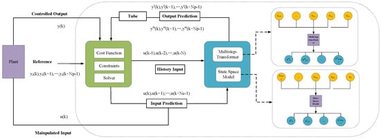
Figure 1. Model predictive control with neural network.

Schematic of the proposed Trans-Tube-MPC structure. Notation: Np: prediction horizon; Nc: control horizon; ys: setpoint; ym: measured output; u: manipulated input; y: controlled output (e.g., temperature in °C, CO concentration in %). The input on the left side of the diagram is the future reference trajectory $y_p(k)y_p(k+1)\dots y_p(k+Np-1)$. These are the desired output values of the system for the next Np time steps.

Predictive model combines state space model and multi-step transformer to predict future outputs $y_p(k)y_p(k+1)\dots y_p(k+Np-1)$ based on current and future inputs $u(k)u(k+1)\dots u(k+Nc-1)$.

Cost function includes the objective function used for optimization, typically aimed at minimizing errors and control energy. Contains the physical and operational constraints that the system must satisfy. Solves the optimization problem to find the optimal control input sequence $u(k)u(k+1)\dots u(k+Nc-1)$.

The controlled output y(k) is the actual output of the system, fed back to the predictive controller. The manipulated input u(k) is the control signal calculated by the controller and applied to the actual system (Plant). The plant is the actual physical system that receives the manipulated input u(k) and generates the controlled output y(k).

The working principle of the entire process is as follows: The predictive controller receives the reference trajectory and uses the predictive model to calculate future outputs. Based on the predicted outputs and reference values, the solver optimizes the cost function and considers constraints to calculate the optimal control input sequence. The current control input u(k) is applied to the plant. The plant generates the controlled output y(k) and feeds it back to the predictive controller. The predictive controller repeats these steps at each sampling period to achieve the goal of tracking the reference trajectory in the future.

3.1. State Space Model

MPC is a control algorithm rooted in predictive modeling. This modeling approach relies on historical data related to the control object to forecast process outputs at a future time. The predictive model has a broad range of applications and is not constrained by specific structural forms; rather, it focuses on functional roles that enable accurate predictions of future control object outputs. These predictive models can be derived from state equations, transfer functions, and other traditional mathematical control models. For linear stable systems, predictive models can be established through finite step response or finite impulse response methodologies.

As the loss function aims to optimize changes in the input vectors, we initially perform some transformations to substitute the input vectors in the state equations with the alterations in the input. Let:

$$\begin{gathered} \Delta u(k)=u(k)-u(k-1) \\ \Delta {\mathit{x}}_{\mathit{m}}(\mathit{k}+1)={\mathit{A}}_{\mathit{m}}\Delta {\mathit{x}}_{\mathit{m}}(\mathit{k})+{\mathit{B}}_{\mathit{m}}\Delta \mathit{u}(k-1) \\ x(k)={\left[x_m{(k)}^{T}y(k)\right]}^T \end{gathered}$$

(6)

Then:

$$\left\{\begin{array}{l}\Delta y(k+1)=C_m{A}_m\Delta x(k)+C_m{B}_m\Delta u(k)\hfill \\ y(k+1)=y(k)+C_m{A}_m\Delta x(k)+C_m{B}_m\Delta u(k)\hfill \end{array}\right.$$

(7)

Written in compact form

$$\left[\begin{array}{c}\Delta x_m(k+1)\\ y(k+1)\end{array}\right]=\left[\begin{array}{cc}{A}_m& o_m^T\\ C_m{A}_m& 1\end{array}\right]\left[\begin{array}{c}\Delta x_m(k)\\ y(k)\end{array}\right]+\left[\begin{array}{c}{B}_m\\ C_m{B}_m\end{array}\right]\Delta u(k)y(k)=\left[\begin{array}{c}{o}_{m}1\end{array}\right]\left[\begin{array}{c}\Delta x_m(k)\\ y(k)\end{array}\right]$$

Obviously, the new state space equation is:

$$\left\{\begin{array}{l}x(k+1)=Ax(k)+Bu(k)\hfill \\ y(k)=Cx(k)\hfill \end{array}\right.$$

(8)

where

$$A=\left[\begin{array}{cc}{A}_m& o_m^T\\ C_m{A}_m& 1\end{array}\right], B=\left[\begin{array}{c}{B}_m\\ C_m{B}_m\end{array}\right], C=\left[o_{m}1\right], x(k)=\left[{\displaystyle \frac{\Delta x_m(k)}{y(k)}}\right]$$

3.2. Multi-Step Neural Network

The Transformer model consists of an encoder and a decoder, each of which includes multiple layers of self-attention mechanisms and feedforward neural networks. The encoder is used to encode the input sequence into context vectors, while the decoder uses these context vectors to generate the target sequence.

Assuming the input sequence is $X=(x_1,x_2,\dots ,x_T)$, the goal is to predict $Y=(y_{T+1},y_{T+2},\dots ,y_{T+k})$, where T is the length of the known historical data, and K is the prediction horizon. For each prediction step k, the decoder output ${\widehat{Y}}_{T+K}$ is based on the prediction from the previous step ${\widehat{Y}}_{T+K-1}$. In the Transformer, the decoder’s input is the prediction result or the true target value from the previous time step. This core part allows the model to process all positions in the input sequence simultaneously, with each “head” focusing on different parts of the input. The Transformer model used in this work consists of 6 encoder and decoder layers, 8 attention heads, a hidden dimension of 512, and a feedforward dimension of 2048. It was trained using the Adam optimizer with L2 regularization, a batch size of 32, and a learning rate of 1 × 10⁻⁴.

$$\begin{array}{l}\mathrm{Attention}(Q,K,V)=\mathrm{softmax}\left({\displaystyle \frac{Q{K}^T}{\sqrt{d_k}}}\right)V\\ \mathrm{MultiHead}(Q,K,V)=\mathrm{Concat}\left({\mathrm{head}}_1,\dots ,{\mathrm{head}}_h\right)W^O\\ {\mathrm{head}}_i=\mathrm{Attention}\left(Q{W}_i^Q,K{W}_i^K,V{W}_i^V\right)\end{array}$$

(9)

where $\mathrm{Q}, \mathrm{K}, \mathrm{V}$ are the queries, keys, and values, which are linear transformations of the input, $Q{W}_i^Q,K{W}_i^K,V{W}_i^V$ are learnable parameters.

Since the Transformer lacks the inherent ability to process sequential data, positional encoding is used to incorporate temporal information into the sequence. A common method is using a combination of sine and cosine functions:

$$\begin{array}{l}P{E}_{pos,2i}=\sin \left({\displaystyle \frac{pos}{{10000}^{2i/d_{\mathrm{model}}}}}\right)\\ P{E}_{pos,2i+1}=\cos \left({\displaystyle \frac{pos}{{10000}^{2i/d_{\mathrm{model}}}}}\right)\end{array}$$

(10)

where pos is the position in the sequence, i is the dimension index, $d_{\mathrm{model}}$ is the model dimension. In multi-step prediction, the output at each time step is determined by the output from the previous time step and the context information.

The direct method directly predicts multiple future time steps as shown in Figure 2. In this method, each time step prediction is carried out independently. For the input sequence $y=\{y_1,y_2,\dots ,y_T\}$, the Transformer encoder transforms the input sequence into hidden representations $\mathrm{z}$, and then predicts each future time step through different decoder heads or different decoding steps.

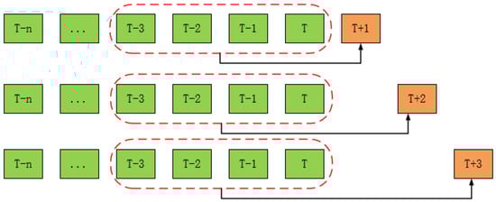
Figure 2. Transformer Direct Method.

The input sequence $y=\{y_1,y_2,\dots ,y_T\}$ is passed through the Transformer encoder to generate the hidden representations $\mathrm{z}$

$$Z=\mathrm{TransformerEncoder}(y)$$

(11)

For each future time step $\mathrm{t} + \mathrm{j}$ where $j=1,2,\dots ,H$ a decoder head or different linear layers $w_{\mathrm{out}}^{(i)}$ of the same decoder are used to generate the predicted values ${\widehat{x}}_{T+j}$

$$\begin{array}{l}{\widehat{y}}_{T+1}=W_{\mathrm{out}}^{(1)}\cdot \mathrm{TransformerDecoder}(Z)\\ {\widehat{y}}_{T+2}=W_{\mathrm{out}}^{(2)}\cdot \mathrm{TransformerDecoder}(Z)\\ {\widehat{y}}_{T+H}=W_{\mathrm{out}}^{(H)}\cdot \mathrm{TransformerDecoder}(Z)\end{array}$$

(12)

3.3. Trans-Tube-MPC

The Trans-Tube-MPC combines the linear state-space model with the multi-step predictive model to optimize control inputs, ensuring the system output closely follows the reference value. The “tube” refers to a guaranteed and adjusted bounded area around the nominal trajectory to ensure robustness against disturbances and model errors. To enhance robustness against model mismatch, we introduce a dynamic tube constraint governed by the prediction discrepancy between the Transformer and state-space model. Assuming $\mathrm{Nc}$ for the control step and $\mathrm{Np}$ for the prediction step. The linear state-space model and the multi-step predictive model are shown as below:

$$\left\{\begin{array}{l}x(k+1)=Ax(k)+B\Delta u(k)\hfill \\ y(k)=Cx(k)+D\Delta u(k)\hfill \\ \widehat{y}(k)=f(u_{k-i{N}_c+1:k},y_{k-i{N}_c+1:k})\hfill \end{array}\right.$$

(13)

Predicting the future x state and y state of the system within the prediction interval

$$\begin{array}{l}x(k_i+N_p|k_i)=A^{N_p}x(k_i)+A^{N_p-1}B\Delta u(k_i)+\\ A^{N_p-2}B\Delta u(k_i+1)+\dots +A^{N_p-N_c}B\Delta u(k_i+N_c-1)\end{array}$$

(14)

$$\begin{array}{l}y(k_i+N_p|k_i)=C{A}^{N_p}x(k_i)+C{A}^{N_p-1}B\Delta u(k_i)+\\ C{A}^{N_p-2}B\Delta u(k_i+1)+\dots +C{A}^{N_p-N_c}B\Delta u(k_i+N_c-1)\end{array}$$

(15)

where $N_p=1,2,\dots ,N_p$, and Let

$$\begin{gathered} \Delta U=\left[\Delta u{(k_i)}^T\Delta u{(k_i+1)}^T\dots \Delta u{(k_i+N_c-1)}^T\right], \\ Y=\left[y{(k_i+1|k_i)}^{T}y{(k_i+2|k_i)}^T\dots y{(k_i+N_p|k_i)}^T\right], \\ \widehat{Y}=\left[\widehat{y}{(k_i+1|k_i)}^T\widehat{y}{(k_i+2|k_i)}^T\dots \widehat{y}{(k_i+N_p|k_i)}^T\right] \end{gathered}$$

Then

$$Y=Fx(k_i)+\Phi \Delta U$$

(16)

where

$$F=\left[\begin{array}{c}CA\\ C{A}^2\\ C{A}^3\\ ⋮\\ C{A}^{N_p}\end{array}\right] \Phi =\left[\begin{array}{cccc}CB& 0& \dots & 0\\ CAB& CB& \dots & 0\\ C{A}^{2}B& CAB& \dots & 0\\ ⋮& ⋮& \ddots & ⋮\\ C{A}^{N_p-1}B& C{A}^{N_p-2}B& \dots & C{A}^{N_p-N_c}B\end{array}\right]$$

where x and u represent the system’s state and control input, respectively. $\mathrm{y}\left(\mathrm{k}\right)$ is the prediction from the state space model, and $\widehat{y}(k)$ is the prediction based on the multi-step model.

To enhance robustness against model mismatch, we introduce a dynamic tube constraint governed by the prediction discrepancy between the Transformer and state-space model. Define the Tube width at step k as:

$$\Delta (k)=\alpha \Delta (k-1)+(1-\alpha )\Vert \widehat{y}(k)-y(k){\Vert }_2$$

(17)

where α determines the constraint adjustment speed. This width modulates the admissible control input range: $u_{\min }+\Delta (k)\le u(k)\le u_{\max }-\Delta (k)$.

The control objective is to minimize tracking errors, input variations, and tube constraint penalties:

$$J={\displaystyle \sum _{i=1}^{N_p}\left(\Vert y_{\mathrm{ref}}-y^{(i)}{\Vert }_Q^2+\Vert \Delta u^{(i)}{\Vert }_R^2\right)}+\lambda {\displaystyle \sum _{j=1}^{N_c}\Delta }{(j)}^2$$

(18)

where $q\ge 0$, $R\ge 0$, $\lambda \ge 0$, and $\mathrm{Q}, \mathrm{R}$ are weight matrices, $\lambda$ is the tube penalty coefficient. The smoothing factor α was set to 0.8 to balance historical and current residuals. The tube penalty coefficient $\lambda$ was tuned in the range of 0.05 to 0.2, with 0.1 selected for the final experiments.

Based on the control sequence definition. Equation (18) is reformulated into the standard QP form:

$$J={\displaystyle \frac{1}{2}}\Delta U^{T}H\Delta U+f^T\Delta U+C$$

(19)

where

$\Delta U$: The change in control input. H is The Hessian matrix, representing the coefficient matrix of the quadratic terms. $f$ is The gradient term, representing the coefficient vector of the linear terms. C is the constant term, independent of the control input.

The Hessian matrix H is defined as:

$$H=2\left(B^{T}QB+R\right)$$

(20)

where $\overline{Q}=\mathrm{diag}(Q,\dots ,Q)$ and $\overline{R}=\mathrm{diag}(R,\dots ,R)$. The gradient term $f$ is defined as:

$$f=2B^T\overline{Q}(Y_{\mathrm{ref}}-A{x}_k)$$

(21)

The constant term $C$ is defined as:

$$C=\lambda {\displaystyle \sum {\Delta }^2}(k+i)$$

(22)

Since C is independent of ΔU, it does not affect the optimal solution. The optimal control sequence is derived as:

$$\Delta U^{*}=-H^{1}f$$

(23)

The first control input is applied:

$$u_k=u_{k-1}+\Delta U^{*}[0]$$

(24)

The complete algorithm flow is shown in Algorithm 1.

Algorithm 1. Trans-Tube-MPC

Input: State-space model (A, B, C), Transformer T_θ, Prediction horizon $\mathrm{Np}$, Control horizon $\mathrm{Nc}$  Output: Optimal control sequence U* 1: Initialize:       - Estimate initial state x^_0 via Kalman filter       - Set initial Tube width Δ = 0, smoothing factor α = 0.8, penalty coefficient λ = 0.1 2: for control cycle k = 0,1,…,N_p do 3:        # Feedforward prediction 4:        y_ssm = A x^_k + B u_k 5:        y_trans = T_θ(encode(u_{k − T:k}, y_{k − T:k})) 6:         7:        # Tube constraint update 8:        residual = np.linalg.norm(y_trans − y_ssm, ord = 2) 9:        Δ = α * Δ_prev + (1 − α) * residual 10:      u_min_adj = u_min_nominal + Δ 11:      u_max_adj = u_max_nominal − Δ 12:       13:      # Construct QP problem 14:      H = 2 * (B.T @ $\overline{q}$ @ B + $\overline{R}$) 15:      f = 2 * B.T @ $\overline{q}$ @ (Y_ref − A @ x^_k) 16:      C = λ * np.sum(Δ**2) 18:      # Solve QP 19:       $\Delta U^{*}$ = -np.linalg.inv(H) @ f 20:      u_k = u_prev + $\Delta U^{*}$ [0] 22:      # State update 23:      x^_{k + 1} = kalman_update(A @ x^_k + B @ u_k, y_{k + 1}) 24: end for

4. Experiment

The paper focuses on the temperature control system of a C5 preheater in cement production, verifying the performance of four control algorithms (conventional MPC, Tube-MPC, Trans-MPC, and Tube-Trans-MPC) under model mismatch scenarios. The system transfer function model is defined as shown in Table 1, where the input variable MV is the coal feed to the calciner, and the output variables CV = [CV1, CV2] represent the C5 temperature and CO concentration, respectively. Tp (s), Td(s), Kp, CV1 (°C), CV2 (% CO). The dataset was split into 2/3 for training and 1/3 for validation.

Table 1. Transfer function.

	MV1
CV1	$g_{11}(s)={\displaystyle \frac{20}{1+455\cdot s}}\cdot e^{200s}$
CV2	$g_{21}(s)={\displaystyle \frac{0.2}{1+90\cdot s}}\cdot e^{30s}$

Set the controller’s prediction horizon to 50 and the control horizon to 10. The matrices are defined as Q = [0 0; 0 1], R = [2.5 0; 0 1], S = [0 0; 0 1]. The remaining parameters are set as shown in Table 2:

Table 2. Parameters setting.

	Min	Max	Value	Target	Weight
MV	[15]	[25]	[17]	[18]	[0]
OV	[860, 0]	[880, 0.4]	[860, 0.25]	[870, 0.05]	[1, 0]

The paper employs four algorithms, with their configurations detailed in Table 3.

Table 3. Algorithm Configurations.

Algorithm	Configuration	Key Differences
MPC	Based on nominal state-space model	No disturbance compensation mechanism
Tube-MPC	Fixed Tube boundary	Static robustness constraints, no dynamic adaptation
Trans-MPC	Uses Transformer for disturbance prediction and No Tube constraints	Purely data-driven compensation, lacks stability guarantees
Tube-Trans-MPC	Transformer predictor and dynamic Tube adjustment	Proposed method: dual-mode robust compensation

• MPC: Baseline with two-term quadratic cost: tracking error + input variation
• Tube-MPC: Fixed tube boundary handles bounded uncertainties
• Trans-MPC: Embeds 6-layer Transformer (hidden = 512, feedforward = 2048, 8 attention heads)
• Tube-Trans-MPC: Dual-mode compensation, Transformer-based multi-step disturbance prediction and Tube width adaptation via prediction residuals

In the actual production system of cement, the C5 temperature model is influenced by production and equipment, and due to frequent changes in operating conditions, a variety of process models are generated. Definition of model mismatch levels based on the actual working conditions of cement production, 13 levels of model mismatch (−60% to +60%) are set, with parameter variation rules as shown in Table 4.

Table 4. Model-plant mismatch ratio.

Model-Plant Mismatch Ratio	Kp	Tp	Td
−60%	8	180	80
−50%	10	230	100
−40%	12	270	120
−30%	14	320	140
−20%	16	360	160
−10%	18	410	180
−5%	19	430	190
0%	20	455	200
5%	21	480	210
10%	22	500	220
20%	24	545	240
30%	26	590	260
40%	28	635	280
50%	30	680	300
60%	32	725	320

Calculation Rules

Kp follows linear scaling, Tp scales inversely, and Td scales proportionally, with specific rules defined by the following equations.

$$K_{\mathrm{actual}}=K_{\mathrm{nominal}}\times \left(1+{\displaystyle \frac{\mathrm{mismatch} \mathrm{ratio}}{100}}\right)$$

(25)

$$T_{\mathrm{actual}}={\displaystyle \frac{T_{\mathrm{nominal}}}{1+\frac{\mathrm{mismatch} \mathrm{ratio}}{100}}}$$

(26)

$$T_d^{\mathrm{actual}}=T_d^{\mathrm{nominal}}\times \left(1+{\displaystyle \frac{\mathrm{mismatch} \mathrm{ratio}}{100}}\right)$$

(27)

In the paper, the initial Transformer model was trained using offline data comprising a dataset of approximately 10,000 instances. The data dimensions include MV1, MV2, CV1, and CV2, where MV1, MV2, and CV1 are used as input data, and CV2 is used as output data. Two-thirds of the dataset was used for model training, while the remaining one-third was used for model validation. The parameters were optimized using the Adam optimizer and L2 regularization. In each failure model scenario, comparative tests were conducted using several MPC. The test results are shown in Table 5. All results are based on 5 independent runs. Standard deviations for RMSE were within ±0.3 across all mismatch scenarios.

Table 5. Control results under different case.

Ratio	Peak Value				Overshoot				Rmse
	Tube-Mpc	Trans-Tube-Mpc	Mpc	Trans-Mpc	Tube-Mpc	Trans-Tube-Mpc	Mpc	Trans-Mpc	Tube-Mpc	Trans-Tube-Mpc	Mpc	Trans-Mpc
−60%	878.903	872.629	878.679	872.890	1.02%	0.30%	1.00%	0.33%	4.987	6.040	6.876	6.164
−50%	877.699	874.908	870.654	868.816	0.89%	0.56%	0.08%	No-overshoot	4.818	6.283	6.227	8.867
−40%	883.421	878.389	869.541	869.450	1.54%	0.96%	No-overshoot	No-overshoot	5.549	6.002	6.101	8.016
−30%	880.461	876.208	869.723	874.915	1.20%	0.71%	No-overshoot	0.56%	4.932	5.645	5.309	7.426
−20%	877.660	879.192	877.677	870.659	0.88%	0.88%	1.06%	0.08%	4.699	5.524	7.677	5.843
−10%	873.067	874.934	873.067	874.934	0.35%	0.57%	0.35%	0.57%	4.144	5.060	4.144	5.060
−5%	871.055	871.703	871.055	871.703	0.12%	0.20%	0.12%	0.20%	3.802	4.506	3.802	4.506
0%	870.304	869.934	870.304	869.934	0.04%	No-overshoot	0.04%	No-overshoot	3.838	4.389	3.838	4.389
5%	871.849	870.085	871.849	870.085	0.21%	0.01%	0.21%	0.01%	3.928	4.401	3.928	4.401
10%	873.675	871.389	873.675	871.389	0.42%	0.16%	0.42%	0.16%	4.181	4.452	4.181	4.452
20%	877.771	872.264	877.762	872.264	0.89%	0.26%	0.89%	0.26%	6.076	4.629	6.076	4.629
30%	882.894	873.160	882.324	872.295	1.48%	0.36%	1.42%	0.26%	8.679	4.779	9.044	4.674
40%	886.904	874.797	884.352	871.460	1.94%	0.55%	1.65%	0.17%	10.389	5.049	11.127	5.354
50%	889.261	876.851	884.618	871.980	2.21%	0.79%	1.68%	0.23%	11.315	5.753	11.297	6.279
60%	893.329	879.246	885.296	873.187	2.68%	1.06%	1.76%	0.37%	12.463	6.346	11.908	7.464

From the Table 5, the variation trends of Peak Value, Overshoot, and RMSE for the four methods under different Ratio conditions can be observed. The results indicate that for scenarios with a certain degree of mismatch. To quantitatively assess the impact of different degrees of model mismatch on control effectiveness, the following metrics are used to evaluate control performance [30]. Overshoot is used to evaluate the overshoot of the controlled variable; the smaller the overshoot, the better the system’s disturbance rejection.

$$Overshoot=\left({\displaystyle \frac{C{V}_{\max }-C{V}_{\mathrm{target}}}{C{V}_{\mathrm{target}}}}\right)\times 100\%$$

(28)

$$RMSE=\sqrt{{\displaystyle \frac{{\displaystyle \sum {(CV-C{V}_{\mathrm{target}})}^2}}{N}}}$$

(29)

Under negative Ratio conditions, Trans-Tube-MPC generally exhibits lower Peak Values. For example, at Ratio = −60%, Trans-Tube-MPC achieves 872.629 compared to Tube-MPC’s 878.903, suggesting its enhanced effectiveness in handling large negative disturbances to stabilize the system faster. Concurrently, its Overshoot remains lower (0.30% vs. 1.02% for Tube-MPC). However, Trans-Tube-MPC shows slightly higher RMSE (6.040 vs. 4.987), indicating a potential trade-off between peak suppression and overall error accumulation. Under positive Ratio conditions (e.g., 60%), Trans-Tube-MPC demonstrates superior performance with a Peak Value of 879.246 versus Tube-MPC’s 893.329, along with significantly reduced Overshoot (1.06% vs. 2.68%) and lower RMSE (6.346 vs. 12.463). This confirms Trans-Tube-MPC’s comprehensive advantages in large positive disturbance scenarios.

At Ratio = −50%, Trans-MPC achieves no overshoot versus MPC’s 0.08%, demonstrating its capability to eliminate overshoot in specific cases. However, this comes with increased RMSE (8.867 vs. 6.227), requiring application-specific tolerance evaluation. As the absolute Ratio increases (both positive and negative), Tube-MPC and MPC exhibit significant RMSE growth, while Trans-Tube-MPC and Trans-MPC maintain gentler RMSE increments. Particularly under positive Ratios, Trans-Tube-MPC’s RMSE increase is markedly smaller than Tube-MPC’s, evidencing enhanced robustness through Transformer integration.

At Ratio = 0%, all methods exhibit minimal overshoot with their RMSE approaching the lowest value near zero. Notably, under this disturbance-free condition, Trans-Tube-MPC shows a slightly higher RMSE (4.389) compared to Tube-MPC (3.838), which may indicate the additional computational overhead introduced by its feedback mechanism. Nevertheless, in practical applications where disturbance handling capability holds greater significance, Trans-Tube-MPC demonstrates superior performance.

For a clearer comparison, we chose several cases of model failure as shown in Figure 3, Figure 4 and Figure 5. As shown in Figure 2, under the −60% model-plant mismatch conditions, the four control strategies exhibit marked divergence in performance characteristics. From Figure 3a, although CV1 fluctuates and the system is relatively stable, it still exhibits some fluctuations, indicating that the 60% model-plant mismatch has an impact on the system performance. From Figure 3b, With the Tube-MPC setting, although CV1 is close to the target value of 870, the system fails to fully meet the target due to the difference between the model and the plant. the poor control of CV2 and the large adjustment of MV indicate that this setting is less adaptable in the face of model-plant mismatch. From Figure 3c, Trans-MPC shows better control response and is close to the target value of 870 despite the slightly higher CV1. The larger fluctuation of MV indicates that the system’s adjustment action is more drastic in the case of 60% model-plant mismatch and there is a certain gap in control accuracy. From Figure 3d Trans-Tube-MPC shows a smoother control effect compared to the other settings, with CV1 close to the target value of 870 and CV2 with better stability. The adjustment of MV fluctuates, but the overall performance of the system is more stable in the case of 60% model-plant mismatch.

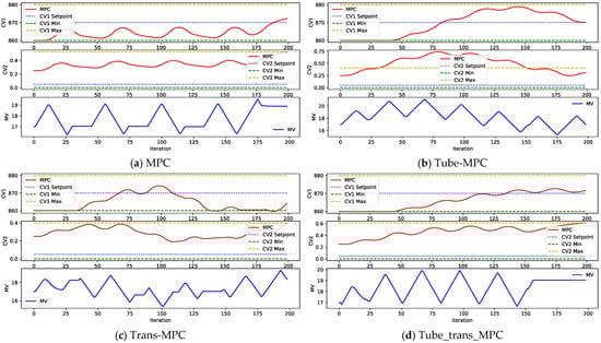
Figure 3. Different MPC model-plant mismatch (−60%). (a) MPC model-plant mismatch. (b) Tube-MPC model-plant mismatch. (c) Trans-MPC model-plant mismatch. (d) Tube_trans_MPC model-plant mismatch.

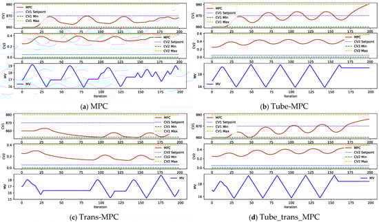
Figure 4. Different MPC model-plant mismatch (−30%). (a) MPC model-plant mismatch. (b) Tube-MPC model-plant mismatch. (c) Trans-MPC model-plant mismatch. (d) Tube_trans_MPC model-plant mismatch.

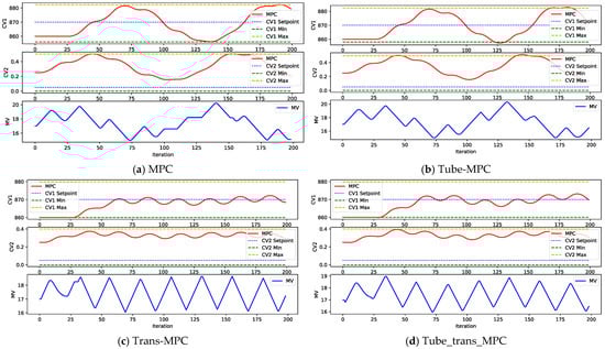
Figure 5. Different MPC model-plant mismatch (+30%). (a) MPC model-plant mismatch. (b) Tube-MPC model-plant mismatch. (c) Trans-MPC model-plant mismatch. (d) Tube_trans_MPC model-plant mismatch.

The Tube-MPC and Trans-Tube-MPC settings converge to a target value of 870 for CV1 in the face of 60% model-plant mismatch, but fluctuate, and the control accuracy of the system decreases. MPC settings have larger overshoots and higher RMSEs despite CV1 being close to the target value, and the control accuracy of the system is poorer. Trans-MPC and Trans-Tube-MPC have a smoother control response, with CV1 close to the target value of 870, relatively small control error, and smoother adjustment of MV.

As shown in Figure 3, under the −30% model-plant mismatch condition, four control strategies exhibited significant performance differences. From Figure 4a, CV1 is close to the target value with good stability, but CV2 fluctuates more, showing some mismatch effects and periodic fluctuations in MV adjustment. From Figure 4b, CV1 is close to the target value, but not quite there, CV2 is poorly controlled, and MV adjustment is large, indicating poor adaptability. From Figure 4c, CV1 is close to the target value but slightly higher, CV2 fluctuates more, MV fluctuates more, and the control accuracy has decreased. From Figure 4d, CV1 is close to the target value, CV2 is stable, MV is adjusted smoothly, showing the best control effect

With the Tube-MPC setting, although CV1 is close to the target value of 870, the system fails to fully meet the target due to the difference between the model and the plant, with poorer control of CV2 and larger MV adjustments, showing poorer adaptability. The Trans-MPC setting is able to keep CV1 close to the target value of 870 better, but due to the larger MV fluctuation, the control accuracy of the system decreases. The Trans-Tube-MPC performs the smoothest, with CV1 close to the target value of 870, better stability of CV2, and smoother adjustment of MV, suggesting that this configuration has the best control effect at 30% model-plant mismatch. Overall, Trans-Tube-MPC performs best in this model-plant mismatch scenario, maintaining the target value and controlling the stability of the other variables better.

As shown in Figure 4, under a 30% model-plant mismatch, Trans-Tube-MPC performs the best, effectively keeping both CV1 and CV2 close to their target values with minimal fluctuations, which reflects its superior control stability. This configuration manages to handle the mismatch without significant deviation, ensuring precise tracking of the setpoints. Trans-MPC, while still performing well, shows noticeable improvements in controlling CV2 compared to other methods, exhibiting fewer and smaller fluctuations, but it does not quite match Trans-Tube-MPC in overall control accuracy and stability.

On the other hand, Tube-MPC and MPC show similar levels of performance, where CV1 remains relatively close to the target, but CV2 experiences larger fluctuations, indicating that the control system is less stable. The MV adjustments are also more frequent and larger in scale, suggesting that these methods are more reactive and less precise in handling the mismatch. Trans-Tube-MPC outperforms the other configurations by providing stronger control, maintaining both CV1 and CV2 with minimal deviation from their setpoints, and ensuring the most stable and precise response under a 30% mismatch scenario. This makes it the most robust choice for handling such mismatches in practical applications.

In conclusion, the experiment compares the performance of different control methods under severe model-plant mismatches (±60%). The results show that the performance of traditional predictive control methods significantly deteriorates when model errors exceed 30%. When the mismatch reaches 60%, the control error of traditional methods reaches 11.9, while the newly developed Tube-Trans-MPC method can stabilize the error between 6.3 and 7.5, demonstrating its stronger ability to handle abnormal situations.

Specifically, Tube-Trans-MPC performs exceptionally well in three areas: Under a 60% severe mismatch, it improves control accuracy by 1.6% to 3.7% compared to regular Tube-MPC (e.g., peak error drops from 893.3 to 879.2), reduces overshoot by 61%, and improves overall error metrics (RMSE) by nearly half. When encountering negative disturbances (e.g., −50% mismatch), it eliminates overshoot, whereas traditional methods still exhibit a 0.08% overshoot. Under common moderate mismatches (±20%), its error is reduced by 21% to 37% compared to using the Transformer method alone.

Hybrid architecture exhibits advantages in typical ±20% mismatch scenarios, reducing control errors by 21–37% compared to standalone Transformer-based control. Subsequent work will validate its generalization capabilities across full-process cement production, with emphasis on long-term stability under complex coupled operational conditions.

5. Conclusions

The paper proposes the Trans-Tube-MPC method, which integrates the temporal modeling capabilities of Transformer with Tube robust constraints to mitigate control performance degradation caused by model-plant mismatches in industrial processes. The core innovation lies in establishing a dynamic compensation loop: the Transformer module employs multi-step attention mechanisms to predict the cumulative impact of disturbances on system states, enabling online correction of predictive model outputs, while the Tube constraints dynamically adjust control boundaries based on real-time errors to suppress overcompensation tendencies of deep learning models. Experimental results demonstrate that under extreme 60% model mismatch, the proposed method achieves a 58% reduction in RMSE compared to conventional MPC and operational safety. Notably, the hybrid architecture exhibits advantages in typical ±20% mismatch scenarios, reducing control errors by 21–37% compared to standalone Transformer-based control. Subsequent work will validate its generalization capabilities across full-process cement production, with emphasis on long-term stability under complex coupled operational conditions. Despite its advantages, the proposed method requires substantial offline training data and computational resources for Transformer inference. Future work will explore lightweight neural architectures, online adaptation strategies, and extended validation in multi-variable and large-scale industrial processes.

References

- Schwenzer, M.; Ay, M.; Bergs, T.; Abel, D. Review on model predictive control: An engineering perspective. Int. J. Adv. Manuf. Technol. 2021, 117, 1327–1349. [Google Scholar] [CrossRef]
- Hu, J.; Shan, Y.; Guerrero, J.M.; Ioinovici, A.; Chan, K.W.; Rodriguez, J. Model predictive control of microgrids–An overview. Renew. Sustain. Energy Rev. 2021, 136, 110422. [Google Scholar] [CrossRef]
- Darby, M.L.; Nikolaou, M. MPC: Current practice and challenges. Control Eng. Pract. 2012, 20, 328–342. [Google Scholar] [CrossRef]
- Schäfer, J.; Cinar, A. Multivariable MPC system performance assessment, monitoring, and diagnosis. J. Process Control 2004, 14, 113–129. [Google Scholar] [CrossRef]
- Sun, Z.; Qin, S.J.; Singhal, A.; Megan, L. Performance monitoring of model-predictive controllers via model residual assessment. J. Process Control 2013, 23, 473–482. [Google Scholar] [CrossRef]
- Kheradmandi, M.; Mhaskar, P. Model predictive control with closed-loop re-identification. Comput. Chem. Eng. 2018, 109, 249–260. [Google Scholar] [CrossRef]
- Drgoňa, J.; Arroyo, J.; Figueroa, I.C.; Blum, D.; Arendt, K.; Kim, D.; Ollé, E.P.; Oravec, J.; Wetter, M.; Vrabie, D.L.; et al. All you need to know about model predictive control for buildings. Annu. Rev. Control 2020, 50, 190–232. [Google Scholar] [CrossRef]
- Chen, Y.; Ierapetritou, M. A framework of hybrid model development with identification of plant-model mismatch. AIChE J. 2020, 66, e16996. [Google Scholar] [CrossRef]
- Xu, X.; Simkoff, J.M.; Baldea, M.; Chiang, L.H.; Castillo, I.; Bindlish, R.; Ashcraft, B. Data-driven plant-model mismatch estimation for dynamic matrix control systems. Int. J. Robust Nonlinear Control 2020, 30, 7103–7129. [Google Scholar] [CrossRef]
- Paulson, J.A.; Santos, T.L.M.; Mesbah, A. Mixed stochastic-deterministic tube MPC for offset-free tracking in the presence of plant-model mismatch. J. Process Control 2019, 83, 102–120. [Google Scholar] [CrossRef]
- Huusom, J.K.; Poulsen, N.K.; Jørgensen, S.B.; Jørgensen, J.B. ARX-model based model predictive control with offset-free tracking. Comput. Aided Chem. Eng. 2010, 28, 601–606. [Google Scholar] [CrossRef]
- Huang, R.; Biegler, L.T.; Patwardhan, S.C. Fast offset-free nonlinear model predictive control based on moving horizon estimation. Ind. Eng. Chem. Res. 2010, 49, 7882–7890. [Google Scholar] [CrossRef]
- Son, S.H.; Narasingam, A.; Kwon, J.S.I. Development of offset-free Koopman Lyapunov-based model predictive control and mathematical analysis for zero steady-state offset condition considering influence of Lyapunov constraints on equilibrium point. J. Process Control 2022, 118, 26–36. [Google Scholar] [CrossRef]
- Wang, J.; Ding, B.; Zhang, S. Multivariable offset-free MPC with steady-state target calculation and its application to a wind tunnel system. ISA Trans. 2020, 97, 317–324. [Google Scholar] [CrossRef]
- González, A.H.; Adam, E.J.; Marchetti, J.L. Conditions for offset elimination in state space receding horizon controllers: A tutorial analysis. Chem. Eng. Process. Process Intensif. 2008, 47, 2184–2194. [Google Scholar] [CrossRef]
- Han, H.G.; Wang, C.Y.; Sun, H.Y.; Yang, H.Y.; Qiao, J.F. Iterative learning model predictive control with fuzzy neural network for nonlinear systems. IEEE Trans. Fuzzy Syst. 2023, 31, 3220–3234. [Google Scholar] [CrossRef]
- Blaud, P.C.; Chevrel, P.; Claveau, F.; Haurant, P.; Mouraud, A. ResNet and PolyNet based identification and (MPC) control of dynamical systems: A promising way. IEEE Access 2022, 11, 20657–20672. [Google Scholar] [CrossRef]
- Lanzetti, N.; Lian, Y.Z.; Cortinovis, A.; Dominguez, L.; Mercangöz, M.; Jones, C. Recurrent neural network based MPC for process industries. In Proceedings of the 2019 18th European Control Conference (ECC), Naples, Italy, 25–28 June 2019; pp. 1005–1010. [Google Scholar]
- Wu, Z.; Rincon, D.; Christofides, P.D. Process structure-based recurrent neural network modeling for model predictive control of nonlinear processes. J. Process Control 2020, 89, 74–84. [Google Scholar] [CrossRef]
- Chu, J.Z.; Tsai, P.F.; Tsai, W.Y.; Jang, S.S.; Shieh, S.S.; Lin, P.H.; Jiang, S.J. Multistep model predictive control based on artificial neural networks. Ind. Eng. Chem. Res. 2003, 42, 5215–5228. [Google Scholar] [CrossRef]
- Lu, C.H.; Tsai, C.C. Generalized predictive control using recurrent fuzzy neural networks for industrial processes. J. Process Control 2007, 17, 83–92. [Google Scholar] [CrossRef]
- Zhang, T.; Feng, G.; Zeng, X.J. Output tracking of constrained nonlinear processes with offset-free input-to-state stable fuzzy predictive control. Automatica 2009, 45, 900–909. [Google Scholar] [CrossRef]
- Khodarahmi, M.; Maihami, V. A review on Kalman filter models. Arch. Comput. Methods Eng. 2023, 30, 727–747. [Google Scholar] [CrossRef]
- Urrea, C.; Agramonte, R. Kalman filter: Historical overview and review of its use in robotics 60 years after its creation. J. Sens. 2021, 2021, 9674015. [Google Scholar] [CrossRef]
- Feng, S.; Li, X.; Zhang, S.; Jian, Z.; Duan, H.; Wang, Z. A review: State estimation based on hybrid models of Kalman filter and neural network. Syst. Sci. Control Eng. 2023, 11, 2173682. [Google Scholar] [CrossRef]
- Transformer, C.G.P.; Zhavoronkov, A. Rapamycin in the context of Pascal’s Wager: Generative pre-trained transformer perspective. Oncoscience 2022, 9, 82. [Google Scholar] [CrossRef]
- Han, K.; Xiao, A.; Wu, E.; Guo, J.; Xu, C.; Wang, Y. Transformer in transformer. Adv. Neural Inf. Process. Syst. 2021, 34, 15908–15919. [Google Scholar] [CrossRef]
- Han, K.; Wang, Y.; Chen, H.; Chen, X.; Guo, J.; Liu, Z.; Tang, Y.; Xiao, A.; Xu, C.; Xu, Y.; et al. A survey on vision transformer. IEEE Trans. Pattern Anal. Mach. Intell. 2022, 45, 87–110. [Google Scholar] [CrossRef]
- Bi, Y.; Ji, Y. Parameter estimation of fractional-order Hammerstein state space system based on the extended Kalman filter. Int. J. Adapt. Control Signal Process. 2023, 37, 1827–1846. [Google Scholar] [CrossRef]
- Feng, Z.; Chen, J.; Xiao, W.; Sun, J.; Xin, B.; Wang, G. Learning Hybrid Policies for MPC with Application to Drone Flight in Unknown Dynamic Environments. arXiv 2024, arXiv:2401.09705. [Google Scholar] [CrossRef]
Disclaimer/Publisher’s Note: The statements, opinions and data contained in all publications are solely those of the individual author(s) and contributor(s) and not of MDPI and/or the editor(s). MDPI and/or the editor(s) disclaim responsibility for any injury to people or property resulting from any ideas, methods, instructions or products referred to in the content. |
© 2025 by the authors. Licensee MDPI, Basel, Switzerland. This article is an open access article distributed under the terms and conditions of the Creative Commons Attribution (CC BY) license (https://creativecommons.org/licenses/by/4.0/).