Physics-Informed Neural Modeling of 2D Transient Electromagnetic Fields

Abstract

Electromagnetic wave propagation in complex environments demands accurate yet efficient modeling techniques. This study introduces a physics-informed neural network (PINN) framework for two-dimensional transient electromagnetic analysis, where Helmholtz equations are directly incorporated into the loss function. The model learns spatiotemporal field evolution without relying on spatial discretization or labeled data. Various excitation and material conditions are examined, including single and dual Gaussian sources in both free space and inhomogeneous regions with dielectric and conducting inclusions. Through this formulation, the network captures key wave phenomena such as propagation, reflection, and scattering with high precision. Validations against finite-difference time-domain (FDTD) simulations confirm strong agreement in both temporal and spatial field distributions. The results demonstrate that the proposed PINN provides an effective, mesh-free alternative for modeling electromagnetic wave dynamics, offering scalability for complex and data-sparse scenarios.

1. Introduction

In recent years, physics-informed learning has emerged as a transformative paradigm for scientific computing, bridging the gap between traditional numerical solvers and data-driven machine intelligence [1,2,3,4]. Unlike purely data-driven neural models that require extensive labeled datasets, physics-constrained networks leverage the governing physical laws as intrinsic learning guidance, allowing them to generalize even under sparse or incomplete observations. This paradigm shift has initiated a wave of research efforts aimed at developing neural architectures capable of faithfully capturing complex spatiotemporal dynamics governed by partial differential equations (PDEs).

Building upon this paradigm, physics-informed learning has been actively extended to a variety of domains where the governing physics are expressed by coupled PDE systems. Applications span fluid dynamics [5], heat transfer [6], structural mechanics [7], and seismic wave propagation [8], where the approach enables accurate reconstruction of hidden states from sparse measurements while ensuring physical consistency. Within this context, electromagnetic (EM) field modeling has become one of the most challenging yet promising frontiers [9,10,11,12,13,14,15]. The governing Maxwell’s equations present strongly coupled, high-dimensional systems characterized by multiscale behaviors and intricate boundary interactions. Capturing such phenomena through deep learning requires not only embedding physical constraints into the training process but also designing architectures that preserve the underlying field symmetries and boundary continuity. Accordingly, recent studies have explored diverse strategies—including adaptive loss weighting, domain decomposition, and hybrid formulations that integrate neural operators with physics-based regularization—to enhance the robustness and accuracy of physics-informed frameworks [16,17,18,19].

Despite these advances, most existing approaches have been limited to simplified or idealized scenarios such as homogeneous media, single-source excitations, or steady-state fields. The accurate representation of transient EM interactions, particularly in the presence of spatially varying permittivity and multiple concurrent sources, remains an open challenge. Addressing this problem requires a framework that can flexibly represent coupled field components, maintain temporal consistency, and adapt to discontinuous material transitions without explicit meshing or re-gridding. These needs motivate the aims to develop a time-domain physics-informed neural model capable of resolving multi-source EM wave propagation in two-dimensional inhomogeneous media.

In this paper, we present a physics-informed neural network (PINN) framework for modeling two-dimensional transient electromagnetic (EM) wave propagation in both free-space and inhomogeneous media. The proposed model incorporates the time-domain Helmholtz formulation as the governing PDE, enabling simultaneous representation of coupled electric and magnetic field components. To assess its applicability in complex environments, the framework is applied to scenarios involving inhomogeneous domains containing dielectric blocks with strong permittivity contrast, demonstrating its capability to resolve complex wave interactions within composite media. The model is further examined under multiple source configurations—including single and dual Gaussian excitations—to assess its ability to capture nonlinear field superposition and interference effects. Moreover, unlike prior research, our model can predict wave propagation even under configurations including multiple scatterers (i.e., dielectric blocks, conducting bodies). Quantitative comparisons with conventional finite-difference time-domain (FDTD) simulations are performed to validate its accuracy and generalization performance. While previous studies have demonstrated the potential of PINNs for electromagnetic modeling, the present work distinguishes itself by accurately resolving transient field dynamics in two-dimensional environments with multiple concurrent sources and strongly contrasting materials.

2. Architecture of PINN Framework

Here, a two-dimensional transverse magnetic (TM_z) configuration is considered, where EM wave behavior can be described by a single electric field component ($E_z$), governed by the time-domain Helmholtz equation:

$${\displaystyle \frac{{\partial }^2{E}_z}{\partial t^2}}={\displaystyle \frac{1}{\sqrt{{\epsilon }_0{\epsilon }_r(x,y){\mu }_0{\mu }_r(x,y)}}}\left({\displaystyle \frac{{\partial }^2{E}_z}{\partial x^2}}+{\displaystyle \frac{{\partial }^2{E}_z}{\partial y^2}}\right),$$

(1)

where ${\epsilon }_0$ and ${\mu }_0$ denote the vacuum permittivity and permeability, respectively, while ${\epsilon }_r(x,y)$ and ${\mu }_r(x,y)$ represent their spatially varying relative distributions. The proposed PINN architecture, shown schematically in Figure 1, takes the spatiotemporal coordinates $(x,y,t)$ as input and predicts the scalar electric field $E_z(x,y,t)$. The loss function consists of three major components corresponding to the initial, boundary, and PDE constraints.

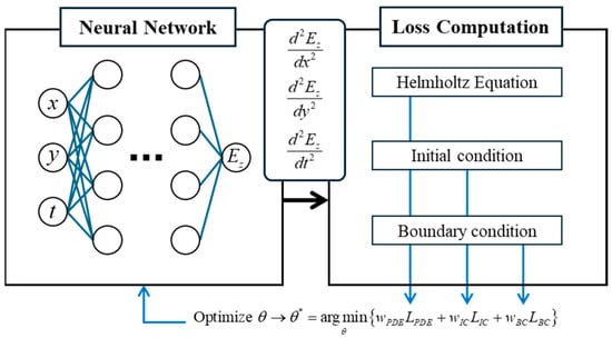
Figure 1. Schematic representation of the PINN framework. Here, ${\theta }^{\ast }$ denotes the optimized value obtained by minimizing the total loss.

The initial condition loss ensures that the predicted field matches the given initial distribution at t = 0. It is defined as

$$L_{IC}={\displaystyle \frac{1}{N_{IC}}}{\displaystyle \sum _{i=1}^{N_{IC}}{\left[{\widehat{E}}_z(x,y,0)-E_z(x,y,0)\right]}^2},$$

(2)

where ${\widehat{E}}_z$ represents the network prediction, and $N_{IC}$ is the number of sampled points at the initial plane.

As for the boundary conditions, the Neumann boundary conditions are imposed on all edges of the computational domain, enforcing $\partial E_z/\partial x=0$ and $\partial E_z/\partial y=0$. These constraints are implemented through the boundary loss term:

$$L_{BC}={\displaystyle \frac{1}{N_{BC}}}{{\displaystyle \sum _{i=1}^{N_{BC}}\left[\frac{\partial {\widehat{E}}_{zi}}{\partial x}\right]}}^2+{\displaystyle \frac{1}{N_{BC}}}{{\displaystyle \sum _{i=1}^{N_{BC}}\left[\frac{\partial {\widehat{E}}_{zi}}{\partial y}\right]}}^2,$$

(3)

where $N_{Bx}$ and $N_{By}$ denote the number of boundary points sampled along the x- and y-directions, respectively.

The PDE residual term enforces the governing time-domain Helmholtz equation across the full spatiotemporal domain:

$$L_{PDE}={\displaystyle \frac{1}{N_{PDE}}}{\displaystyle \sum _{i=1}^{N_{PDE}}\left[\frac{{\partial }^2{\widehat{E}}_{zi}}{\partial t^2}-\right.}{\left.{\left({\displaystyle \frac{c}{\sqrt{{\epsilon }_r(x_i,y_i){\mu }_r(x_i,y_i)}}}\right)}^2\left({\displaystyle \frac{{\partial }^2{\widehat{E}}_{zi}}{\partial x^2}}+{\displaystyle \frac{{\partial }^2{\widehat{E}}_{zi}}{\partial y^2}}\right)\right]}^2.$$

(4)

Here, $N_{PDE}$ is the number of collocation points distributed throughout the computational domain. Therefore, the total loss function combines all three components in a weights summation to ensure simultaneous satisfaction of the governing equation and all physical constraints:

$$L_{total}=w_{IC}{L}_{IC}+w_{BC}{L}_{BC}+w_{PDE}{L}_{PDE},$$

(5)

In all experiments, unit weights are employed, i.e., $w_{IC}=w_{BC}=w_{PDE}=$ 1, so that each component contributes equally to the optimization. This composite objective enables the network to learn the temporal evolution of wave propagation while maintaining consistency with both the initial and boundary conditions.

To initiate transient field evolution, a Gaussian pulse is applied as the external excitation source. Both single and dual Gaussian excitations are considered to examine the framework’s ability to capture superposition and interference effects. Four distinct simulation configurations are designed to comprehensively evaluate the proposed model: (1) free-space with a single Gaussian source, (2) free-space with dual Gaussian sources, (3) inhomogeneous media containing two dielectric blocks excited by a single Gaussian source, and (4) a mixed medium consisting of one dielectric and one conductive block under a single Gaussian source. These cases are selected to progressively increase the complexity of the propagation environment—from simple linear interference in homogeneous media to strongly contrasting materials that induce scattering, reflection, and absorption effects. For each configuration, 10,000 randomly sampled points are used for both the initial and boundary conditions. The PDE collocation points ($N_{PDE}$) are sampled by randomly selecting spatial coordinates $(x,y)$ in the domain, whereas the temporal axis is uniformly sampled with $\alpha$ points from $t\in [0,t_{\max }]$, as depicted in Figure 2. The temporal sampling density, controlled by the parameter $\alpha$, varies according to the complexity of each configuration (see Table 1). To avoid unnecessary over-parameterization, the parameters listed in Table 1 were chosen based on preliminary convergence tests carried out for each configuration. The reported numbers of hidden layers and training epochs correspond to the smallest values for which the training curves stabilized, and the predicted fields visually matched the reference solution across the entire spatiotemporal domain. Although further increasing the depth or the number of epochs can lead to slightly improved predictions, the additional computational cost was not justified by the marginal gain. Likewise, the temporal sampling parameter $\alpha$ was determined by gradually increasing the number of time slices used during training and selecting the minimum value that still yielded accurate reconstructions for each configuration, thereby balancing prediction quality and efficiency.

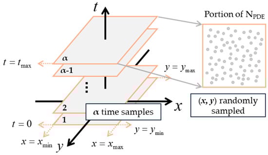
Figure 2. Schematic representation of sampling strategy for PINN training. Here, $\alpha$ denotes the number of temporal samples used during training, and N_PDE denotes the number of PDE collocation points in the interior of the spatiotemporal domain.

Table 1. Network settings for each configuration, including source type and environment.

Configuration	# of Neurons	# of Hidden Layers	Epoch	α/NPDE
Free-space/ Single Gaussian	64	5	5000	26/39,000
Free-space/ Dual Gaussian	64	10	10,000	51/40,800
Inhomogeneous (2 dielectric blocks)/ Single Gaussian	64	15	15,000	101/50,500
Inhomogeneous (dielectric block + conductor)/ Single Gaussian	64	20	15,000	101/50,500

All hidden layers use the hyperbolic tangent (tanh) activation function, and the model is trained using the Adam optimizer with a fixed learning rate of 5 × 10⁻⁴. The network weights are initialized with the Glorot (Xavier) scheme, and full-batch gradient descent is adopted, i.e., all training samples are used in each optimization step without mini-batching. No additional explicit regularization, such as weight decay or dropout, is applied in the present study. All training is performed on Google Colab using Tensorflow 2 with an Nvidia L4 GPU backend.

3. PINN Prediction Results

In this section, the predictive performance of the proposed PINN is evaluated under multiple configuration settings. The simulations are conducted within a temporal range of $t\in [0,10]$ ns and a spatial domain of $x,y\in [-5,5]$ m. To comprehensively assess both the accuracy and generalization capability of the model, four prediction scenarios are examined under two distinct environments: free-space and spatially inhomogeneous media. The resulting PINN predictions are quantitatively compared with reference data obtained from the conventional finite-difference time-domain (FDTD) method to evaluate their agreement in both amplitude and phase. This comparison allows the assessment of how well the proposed framework reproduces the spatiotemporal dynamics of electromagnetic fields and ensures physical consistency across different propagation conditions.

Before presenting the detailed field FDTD scheme used to generate reference data. The reference solution is obtained by numerically solving (1) on the same spatial domain ($x,y\in [-5,5]$ m) and temporal range ($t\in [0,10]$ ns) as used in the PINN framework. The domain is discretized by a uniform Cartesian grid with $n_x\times n_y$ nodes and spatial steps $\Delta x$ and $\Delta y$, while time is advanced with a uniform step $\Delta t$ over $n_t$ time levels. The time step $\Delta t$ is chosen sufficiently small to satisfy the Courant stability condition associated with the two-dimensional scheme. The initial condition corresponds to a localized Gaussian producing a transient, spatially confined excitation around the source location. At the outer boundary of the domain, homogeneous Neumann conditions are imposed. The resulting spatiotemporal field samples from this FDTD-type solver are used as ground-truth reference data for the quantitative comparison with the proposed PINN predictions in the following subsections.

3.1. Field Prediction in a Free-Space Environment

To verify the baseline performance of the proposed PINN, wave propagation in free space excited by a single Gaussian pulse is first examined. The excitation is centered at (0, 2), producing a localized transient electric field with symmetric spatial distribution given by

$$E_z(x,y,0)=\exp \left(-{\displaystyle \frac{x^2}{0.5}}\right)\cdot \exp \left(-{\displaystyle \frac{{\left(y-2\right)}^2}{0.5}}\right).$$

(6)

For this configuration, the PINN model employs a fully connected neural network composed of five hidden layers with 64 neurons per layer and is trained for 5000 epochs, as summarized in Table 1. The temporal domain during training is discretized into 26 uniform time steps, whereas the prediction is carried out on a denser temporal grid of 501 points—corresponding to only 5% of the time samples used for training and 95% for prediction. Among these time samples, representative training planes at t = 0, 5, 10 ns are shown in Figure 3a to illustrate the spatiotemporal evolution of the field. To evaluate the model’s generalization ability, additional predictions are generated at unseen intermediate time planes (t = 3, 6, 9 ns), as depicted in Figure 3b.

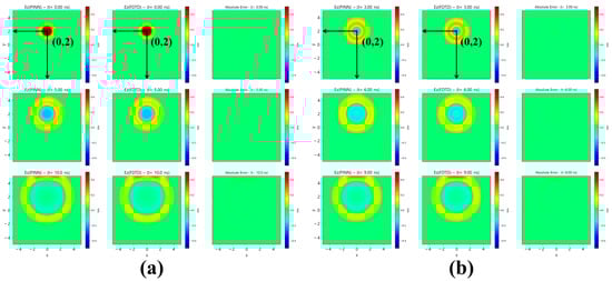
Figure 3. Comparison between predicted and reference field distributions in free space for a single Gaussian source. From left to right, each panel shows the PINN prediction, the FDTD reference, and the absolute error: (a) temporal planes used during training; (b) temporal planes not included in training (unseen temporal planes).

The visual comparisons demonstrate that the wavefronts predicted by the PINN closely follow the FDTD reference across the entire temporal range. Even for the intermediate time steps not included in training, the spatial field distributions exhibit consistent circular symmetry and amplitude decay, indicating that the network successfully captures the underlying wave dynamics rather than memorizing discrete instances. The absolute error maps further confirm that the deviations between the two methods remain negligibly small throughout the domain, even near the expanding edges of the wavefront. This observation highlights the robustness of the proposed framework in preserving both phase continuity and amplitude accuracy during temporal extrapolation. Such performance verifies that the PINN not only learns the spatial propagation characteristics of transient EM waves but also maintains physical fidelity when predicting unseen temporal states. Overall, this result establishes that the proposed model achieves high accuracy and strong generalization capability for single-source free-space propagation, serving as a reliable baseline for more complex multi-source and inhomogeneous scenarios discussed in the following sections.

To further assess the model’s capability in capturing more complex field interactions, a dual-source configuration is examined, where two Gaussian pulses are symmetrically positioned at (−1, −1) and (1, 1). This arrangement generates overlapping wavefronts that interact through constructive and destructive interference, providing a rigorous test of the model’s ability to represent multi-source dynamics. The initial electric field distribution for this configuration is defined as

$$E_z(x,y,0)=\exp \left(-{\displaystyle \frac{{\left(x-1\right)}^2}{0.5}}\right)\cdot \exp \left(-{\displaystyle \frac{{\left(y-1\right)}^2}{0.5}}\right)+\exp \left(-{\displaystyle \frac{{\left(x+1\right)}^2}{0.5}}\right)\cdot \exp \left(-{\displaystyle \frac{{\left(y+1\right)}^2}{0.5}}\right).$$

(7)

To better observe the wave interactions over time, the training is extended to 15 ns only in this case. The PINN model is trained using a neural network with 10 hidden layers, each containing 64 neurons, and optimized for 10,000 epochs. In this case, the temporal domain is uniformly divided into 51 time steps. The inference is performed under the same grid used in the previous case, meaning the model predicted approximately 90% of the temporal planes.

Among these, representative time planes such as t = 0, 5, 10, and 15 ns are shown in Figure 4a, corresponding to the time steps utilized during training. To evaluate the interpolation capability beyond these instances, additional predictions are generated at unseen intermediate time planes (t = 3, 6, 9, and 12 ns), as shown in Figure 4b. The predicted field distributions clearly demonstrate that PINN accurately reproduces the interference fringes and superposition effects between the two sources. Throughout the entire simulation period, including the extended range up to t = 15 ns, the spatial evolution of the wavefronts remains highly consistent with the FDTD reference. The near-zero error level across all frames confirms that the network effectively learns not only the transient propagation but also the reflective behavior at the boundaries governed by the Neumann condition.

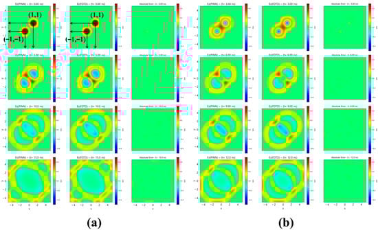
Figure 4. Comparison between predicted and reference field distributions in free space for a dual Gaussian source. From left to right, each panel shows the PINN prediction, the FDTD reference, and the absolute error: (a) temporal planes used during training; (b) temporal planes not included in training (unseen temporal planes).

These results verify that the proposed physics-informed approach maintains physical accuracy in modeling multi-source interactions, successfully predicting both the constructive and destructive interference patterns without any explicit supervision on boundary reflections.

3.2. Field Prediction in Inhomogeneous Media

Accurate prediction of electromagnetic fields in spatially varying media is essential for modeling realistic propagation environments. To examine the robustness of the proposed PINN in such cases, two inhomogeneous configurations are investigated: (i) a dielectric-only case with two inclusions of relative permittivity ${\epsilon }_r$ = 4, and (ii) a mixed medium containing one dielectric and one conducting body.

In the first scenario, two dielectric blocks with relative permittivity ${\epsilon }_r$ = 4 are embedded in an otherwise homogeneous background (${\epsilon }_r$ = 1). The inclusions are positioned asymmetrically within the spatial domain: one block occupies the region $-3\le x\le -2$ and $-2\le y\le 1$, while the other is located at $1\le x\le 3$, $1\le y\le 3$. These regions are indicated by the red dashed rectangles in Figure 5. The initial electric field generated by a single Gaussian pulse centered at the origin, defined as

$$E_z(x,y,0)=\exp \left(-{\displaystyle \frac{x^2}{0.5}}\right)\cdot \exp \left(-{\displaystyle \frac{y^2}{0.5}}\right),$$

(8)

which produces a localized excitation with symmetric spatial spread. This configuration evaluates the model’s ability to capture wave-material interactions and refractions induced by dielectric discontinuities. The PINN is trained using uniformly sampled spatiotemporal points over the entire computational domain with 15 hidden layers and 15,000 training epochs.

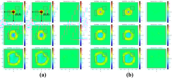
Figure 5. Comparison between predicted and reference field distributions in inhomogeneous media with two dielectric inclusions for a single Gaussian source. From left to right, each panel shows the PINN prediction, the FDTD reference, and the absolute error: (a) temporal planes used during training; (b) temporal planes not included in training (unseen temporal planes).

Figure 5a presents the predicted and reference fields at training time planes (t = 0, 5, 10 ns), while Figure 5b shows the predictions at unseen planes (t = 3, 6, 9 ns). The PINN successfully reproduces the transmitted and reflected wavefronts at both dielectric boundaries, maintaining strong agreement with the FDTD reference across all time steps. The absolute error maps confirm that deviations remain minimal both inside and outside the inclusions, verifying that the model’s interpolation ability even in the presence of sharp permittivity transitions.

The second scenario introduces a more complex environment combining one dielectric inclusion (${\epsilon }_r$ = 4) and one conducting body modeled as a high-${\epsilon }_r$ region with ${\epsilon }_r$ = 2000, effectively producing near-total reflection while maintaining numerical stability. This choice can be physically interpreted by considering the normal-incidence reflection coefficient $\Gamma =\left({\epsilon }_r-1\right)/\left({\epsilon }_r+1\right)$ at the interface between free space and the high-${\epsilon }_r$ region. For ${\epsilon }_r$ = 2000, we obtain $\left|\Gamma \right|\approx$ 0.96, so that more than 95% of the incident field is reflected and only a small fraction is transmitted into the inclusion, closely mimicking the behavior of a good conductor. From a numerical standpoint, representing the conductor as a finite but very large permittivity avoids explicitly imposing a PEC boundary in the scalar time-domain Helmholtz formulation and keeps the problem defined on a single continuous domain, which is advantageous for stable PINN training while still capturing the strong reflection expected at a dielectric–conductor interface. The dielectric block (red dashed lines in Figure 6) is positioned in the upper region ($-3\le x\le 0$, $1\le y\le 2$), while the conducting block (red solid lines in Figure 6) is located in $-2\le x\le -2$ and $-3\le y\le -2$. The initial field distribution is defined by the same Gaussian function used in the previous case.

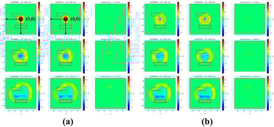
Figure 6. Comparison between predicted and reference field distributions in inhomogeneous media with a dielectric inclusion and a conducting body for a single Gaussian source. From left to right, each panel shows the PINN prediction, the FDTD reference, and the absolute error: (a) temporal planes used during training; (b) temporal planes not included in training (unseen temporal planes).

Figure 6a,b show the predicted fields at training and unseen time planes, respectively. The PINN accurately reconstructs the reflected and refracted wavefronts formed at the dielectric–conductor interfaces, exhibiting strong consistency with the FDTD reference. While localized errors appear along the conductive boundary—where steep phase gradients arise due to the large permittivity discontinuity—the overall wave evolution remains physically consistent and temporally stable. These results confirm that the proposed PINN framework effectively handles high-contrast electromagnetic environments, maintaining prediction accuracy even in the presence of strong reflections and multiple scattering interactions. To further reduce the localized discrepancies near conductive boundaries, more advanced strategies such as interface-aware sampling around high-contrast regions, adaptive reweighting of PDE and boundary losses, or imposing the PEC boundary as a hard constraint could be employed.

A quantitative summary of the overall performance of the proposed framework is provided in Table 2. For each configuration, the table reports the total training time and inference time of the PINN, the FDTD simulation time at the same spatial–temporal resolution, and the mean, maximum, and standard deviation of the relative L2 error over time between the PINN and FDTD fields. As the medium becomes more complex—from free space to inhomogeneous scenarios involving dielectric inclusions and a high-permittivity conductor—the training time increases from 90.3 to 369.8 min, reflecting the higher learning complexity. Nevertheless, the inference time remains on the order of 1–2 s for all cases, which is noticeably shorter than the corresponding FDTD simulation times (approximately 13–15 s). The relative L2 error stays below about 0.2 with standard deviations on the order of 10⁻², indicating that the PINN predictions follow the FDTD reference with good accuracy while maintaining temporally stable behavior. These quantitative results corroborate the visual comparisons in Figure 3, Figure 4, Figure 5 and Figure 6 and clarify the trade-off between the higher offline training cost and the fast mesh-free inference once the network has been trained.

Table 2. A comparison of computational cost and global accuracy between the proposed PINN and the FDTD reference solver for each configuration.

Configuration	PINN (Training/Inference)		FDTD (Simulation)	Relative L2 Error over Time
				Mean	Max	Std
Free-space/ Single Gaussian	90.3 min	1.02 s	13.25 s	8.42 × 10−2	9.98 × 10−2	1.01 × 10−2
Free-space/ Dual Gaussian	174.6 min	1.14 s	13.11 s	1.1 × 10−1	1.26 × 10−1	1.5 × 10−2
Inhomogeneous (2 dielectric blocks)/ Single Gaussian	311.8 min	1.53 s	14.08 s	1.02 × 10−1	1.53 × 10−1	2.34 × 10−2
Inhomogeneous (dielectric block + conductor)/ Single Gaussian	369.8 min	1.66 s	14.5 s	8.88 × 10−2	1.4 × 10−1	3.2 × 10−2

4. Discussion

To better position the proposed framework within the growing body of physics-informed EM modeling, Table 3 summarizes key features of several representative PINN-based approaches for Maxwell’s equations and related systems with the present work. Compared with prior PINN-based EM studies summarized in Table 3, the present model offers several distinctive advantages. First, while most existing works focus on one-dimensional configurations or inverse problems in inhomogeneous media, the proposed framework directly targets forward, transient 2D wave propagation governed by the time-domain Helmholtz equation. This allows us to resolve the full spatiotemporal evolution of the field, rather than only steady-state responses or parameter estimates. Second, our setup systematically explores multiple excitation scenarios, including both single and dual Gaussian sources, so that the model is explicitly tested on wave–wave interaction, interference, and scattering phenomena—features that are not addressed in single-source configurations of previous PINN-based EM studies. Third, the considered environments include strongly inhomogeneous media combining dielectric inclusions and an effectively conducting body, which generate pronounced reflections and complex multi-path behavior.

Table 3. A comparison between prior PINN-based EM works and this work.

Work	Governing Equation	Dimension	Problem Type	Media/Configuration
[13]	Maxwell’s Equation	1D	Forward	Homogeneous and piecewise inhomogeneous media/single source
[18]	Maxwell’s Equation	1D-2D	Inverse	Inhomogeneous media
[19]	2D TM Maxwell’s Equation	2D	Forward + Inverse	Inhomogeneous media with varying single scatterers/single source
[20]	Maxwell + Plasma current Equations	1D	Inverse	Inhomogeneous magnetized plasma
This Work	2D Helmholtz Equation	2D	Foward	Free-space and strongly inhomogeneous media (dielectric inclusions + conducting body)/single + dual sources

Moreover, it is important to understand both the advantages of the PINN-based framework over conventional simulation methods and the aspects in which it can be further improved. Conventional numerical solvers such as FDTD and FEM have long been the standard tools for time-domain EM modeling, but they inevitably incur several practical limitations when fine spatial/temporal resolution or complex material configurations are required. In contrast, the proposed PINN-based framework learns a continuous spatiotemporal representation of the field, which provides a number of qualitative advantages. First, the solution is expressed as a mesh-free neural approximation $E_z$ that is differentiable with respect to both space and time. Once trained, the network can be evaluated at arbitrary locations and time instants without re-discretizing the domain or re-running time-marching iterations. This is particularly beneficial when field values are required only at selected regions or at many different time instants, for example, in parametric sensitivity analysis or post-processing for system-level metrics. Moreover, the PINN formulation naturally embeds the governing PDE and boundary/initial conditions into the loss function, which alleviates the need for designing specialized update schemes, absorbing boundary conditions, or stability criteria such as the Courant–Friedrichs–Lewy (CFL) condition. Traditional FDTD must adopt sufficiently small time steps to guarantee numerical stability, and FEM often requires careful mesh refinement near material interfaces, both of which can lead to prohibitive computational cost in large or strongly inhomogeneous domains. In the present framework, the collocation points can be concentrated in regions of interest (e.g., near dielectric/PEC interfaces or source locations), thereby improving accuracy where it is most needed while keeping the overall number of training samples moderate. This flexibility in sampling, together with the continuous field representation, allows the network to capture wavefront propagation, reflection, and scattering behavior with fewer degrees of freedom than a uniformly discretized grid. Furthermore, the proposed approach is well-suited to scenarios where only partial information about the system is available. Because the network is trained by minimizing a composite loss comprising the PDE residual and a small number of data constraints, it can, in principle, be extended to incorporate measured field samples or boundary observations without modifying the underlying solver. In contrast, integrating experimental data into FDTD/FEM often requires additional model-order reduction or parameter fitting. Although the present study focuses on purely simulation-driven training, a physics-informed formulation provides a natural pathway toward hybrid modeling where numerical and experimental information are fused in a unified framework.

Despite these advantages, the current PINN framework remains essentially a single-scenario solver: for each new excitation or material configuration, the network must be retrained from scratch. A natural extension is therefore to allow the framework to have operator-learning capabilities so that it can approximate a mapping from problem configuration (e.g., source distribution, material profile, or boundary condition) to the corresponding spatiotemporal field response. In this context, physics-informed deep operator networks (Pi-DeepONet) constitute a promising direction, where the trunk network encodes the (x, y, t) coordinates while the branch network encodes the specific excitation and material parameters. With such an operator-based architecture, a single trained model could handle a family of problems, enabling fast prediction of EM wave dynamics across multiple source and dielectric configurations without retraining for each case. Developing and validating this Pi-DeepONet extension for more diverse and practically relevant EM scenarios will be the focus of our future work.

5. Conclusions

In this paper, we investigated the applicability of physics-informed neural networks (PINNs) for modeling time-domain electromagnetic (EM) wave propagation governed by the Helmholtz equation. The proposed framework was examined under various excitation and material configurations, including single and dual Gaussian sources in both free-space and spatially inhomogeneous media. The results confirmed that PINN can accurately reproduce transient EM field evolution and interpolate beyond training instances, achieving close agreement with FDTD simulations even when trained with sparsely sampled temporal data. Although relatively higher errors were observed near sharp dielectric and conductive boundaries, the model consistently captured the essential physical behaviors such as reflection, refraction, and interference. Overall, this study demonstrates the potential of PINNs as a data-free alternative for time-domain EM analysis. Future work will focus on improving generalization capability such that a single trained PINN can adaptively predict field dynamics across multiple excitation and material configurations.

References

- Raissi, M.; Perdikaris, P.; Karniadakis, G. Physics-informed neural networks: A deep learning framework for solving forward and inverse problems involving nonlinear partial differential equations. J. Comp. Phys. 2019, 378, 686–707. [Google Scholar] [CrossRef]
- Lawal, Z.K.; Yassin, H.; Lai, D.T.C.; Che Idris, A. Physics-informed neural network (PINN) evolution and beyond: A systematic literature review and bibliometric analysis. Big Data Cogn. Comput. 2022, 6, 140. [Google Scholar] [CrossRef]
- Raissi, M.; Perdikaris, P.; Karniadakis, G.E. Physics Informed Deep Learning (Part I): Data-driven Solutions of Nonlinear Partial Differential Equations. arXiv 2017, arXiv:1711.10561. [Google Scholar] [CrossRef]
- Karniadakis, G.E.; Kevrekidis, I.G.; Lu, L.; Perdikaris, P.; Wang, S.; Yang, L. Physics-informed machine learning. Nat. Rev. Phys. 2021, 3, 422–440. [Google Scholar] [CrossRef]
- Cai, S.; Mao, Z.; Wang, Z.; Yin, M.; Karniadakis, G.E. Physics-informed neural networks (PINNs) for fluid mechanics: A review. Acta Mech. Sin. 2022, 37, 1727–1738. [Google Scholar] [CrossRef]
- Cai, S.; Wang, Z.; Wang, S.; Perdikaris, P.; Karniadakis, G.E. Physics-Informed Neural Networks for Heat Transfer Problems. J. Heat Transf. 2021, 143, 060801. [Google Scholar] [CrossRef]
- Zhang, E.; Dao, M.; Karniadakis, G.E.; Suresh, S. Analyses of internal structures and defects in materials using physics-informed neural networks. Sci. Adv. 2022, 8, eabk0644. [Google Scholar] [CrossRef] [PubMed]
- Rasht-Behesht, M.; Huber, C.; Shukla, K.; Karniadakis, G.E. Physics-Informed Neural Networks (PINNs) for Wave Propagation and Full Waveform Inversions. J. Geophys. Res. Solid Earth 2022, 127, e2021JB023120. [Google Scholar] [CrossRef]
- Baldan, M.; Di Barba, P.; Lowther, D.A. Physics-informed neural networks for inverse electromagnetic problems. IEEE Trans. Magn. 2023, 59, 7001705. [Google Scholar] [CrossRef]
- Lim, J.; Psaltis, D. MaxwellNet: Physics-driven deep neural network training based on Maxwell’s equations. APL Photon. 2022, 7, 011301. [Google Scholar] [CrossRef]
- Qi, S.; Sarris, C.D. Hybrid physics-informed neural network for the wave equation with unconditionally stable time-stepping. IEEE Antennas Wirel. Propag. Lett. 2024, 23, 1356–1360. [Google Scholar] [CrossRef]
- Chen, M.; Lupoiu, R.; Mao, C.; Huang, D.; Jiang, J.; Lalanne, P.; Fan, J. High speed simulation and freeform optimization of nanophotonic devices with physics-augmented deep learning. ACS Photon. 2022, 9, 3110–3123. [Google Scholar] [CrossRef]
- Zhang, P.; Hu, Y.; Jin, Y.; Deng, S.; Wu, X.; Chen, J. A Maxwell’s equations based deep learning method for time domain electromagnetic simulations. IEEE J. Multiscale. Mu. 2021, 6, 35–40. [Google Scholar] [CrossRef]
- Guan, T.; Chang, S.; Deng, Y.; Xue, F.; Wang, C.; Jia, X. Oriented SAR Ship Detection Based on Edge Deformable Convolution and Point Set Representation. Remote Sens. 2025, 17, 1612. [Google Scholar] [CrossRef]
- Li, Z.; Sun, J.; Fan, Y.; Jin, Y.; Shen, Q.; Trusiak, M.; Cywińska, M.; Gao, P.; Chen, Q.; Zuo, C.; et al. Deep learning assisted variational Hilbert quantitative phase imaging. Opto-Electron. Sci. 2023, 2, 220023. [Google Scholar] [CrossRef]
- Wang, Y.; Zhang, S. Multi-receptive-field physics-informed neural network for complex electromagnetic media. Opt. Mater. Express 2024, 14, 2740–2754. [Google Scholar] [CrossRef]
- Su, Y.; Zeng, S.; Wu, X.; Huang, Y.; Chen, J. Physics-Informed Graph Neural Network for Electromagnetic Simulations. In Proceedings of the 2023 IEEE XXXVth URSI GASS, Sapporo, Japan, 19–26 August 2023. [Google Scholar]
- Piao, S.; Gu, H.; Wang, A.; Qin, P. A domain-adaptive physics-informed neural network for inverse problems of Maxwell’s equations in heterogeneous media. IEEE Antennas Wirel. Propag. Lett. 2024, 23, 2905–2909. [Google Scholar] [CrossRef]
- Liu, H.; Fan, Y.; Ding, F.; Du, L.; Zhao, J.; Sun, C.; Zhou, H. Physics-informed deep model for fast time-domain electromagnetic simulation and inversion. IEEE Trans. Antennas Propag. 2024, 72, 7807–7820. [Google Scholar] [CrossRef]
- Zhang, Y.; Fu, H.; Qin, Y.; Wang, K.; Ma, J. Physics-informed deep neural network for inhomogeneous magnetized plasma parameter inversion. IEEE Antennas Wireless Propag. Lett. 2022, 21, 828–832. [Google Scholar] [CrossRef]
Disclaimer/Publisher’s Note: The statements, opinions and data contained in all publications are solely those of the individual author(s) and contributor(s) and not of MDPI and/or the editor(s). MDPI and/or the editor(s) disclaim responsibility for any injury to people or property resulting from any ideas, methods, instructions or products referred to in the content. |
© 2025 by the authors. Licensee MDPI, Basel, Switzerland. This article is an open access article distributed under the terms and conditions of the Creative Commons Attribution (CC BY) license (https://creativecommons.org/licenses/by/4.0/).