Rolling Bearing Fault Diagnosis via Parallel Heterogeneous Deep Network with Transfer Learning

Abstract

Rolling bearings are critical components in rotating machinery, and their performance degrades over time due to operational wear, which may compromise the safety and efficiency of mechanical systems. Therefore, accurate and timely fault diagnosis of rolling bearings is crucial. In real-world industrial environments, such diagnosis remains challenging owing to complex and varying operating conditions. Conventional single-modality deep learning methods often face limitations and fail to satisfy practical demands. To overcome these challenges, this paper proposes a novel fault diagnosis approach based on a Parallel Heterogeneous Deep Network (PHDN-FD). First, the original vibration signals are segmented according to signal pattern similarity. The continuous wavelet transform (CWT) using the Morse wavelet is applied to convert one-dimensional signal segments into two-dimensional time–frequency representations. Subsequently, each signal segment and its corresponding time–frequency representation are paired to form input data for a dual-branch parallel network. One branch, based on the ConvNeXt architecture, extracts spatial features from the time–frequency images, while the other branch employs a 1D-ResNet to capture temporal features from the raw signal segments. The features from both branches are then fused and fed into a three-layer feedforward neural network for final fault classification. Experimental results on the Case Western Reserve University (CWRU) bearing dataset and Korean Academy of Science and Technology (KAIST) bearing datasets show that the proposed method achieves high diagnostic accuracy even under adverse conditions, such as noise interference, limited training samples, and variable load levels. Moreover, the model exhibits strong cross-load transferability. By effectively integrating multimodal feature representations, the PHDN-FD framework improves both diagnostic accuracy and model robustness in complex operational scenarios, establishing a solid foundation for industrial deployment and demonstrating significant potential for practical applications.

1. Introduction

Rolling bearings are subject to cumulative wear under demanding operating conditions, resulting in progressive performance degradation over time and posing risks to the safety and operational efficiency of mechanical systems [1,2]. As a key component in rotating machinery, rolling bearings are extensively employed across diverse sectors such as industrial manufacturing, transportation, energy production, automotive engineering, and aerospace. Consequently, timely and accurate detection of bearing faults is essential to ensure the safe and reliable operation of mechanical systems [3,4].

Vibration signal analysis is a widely adopted method for detecting faults in rolling bearings. Conventional techniques include the short-time Fourier transform (SFT) [5], wavelet transform (WT) [6], empirical mode decomposition (EMD) [7], and related methods such as the Hilbert–Huang transform [8]. These approaches enable a quantitative assessment of equipment operating states by incorporating established bearing fault indicators, including root mean square, kurtosis, peak value, and crest factor [9]. Chen et al. [10] proposed a method based on multiscale improved envelope spectrum entropy (MIESE), which combines multiscale decomposition with entropy calculation and uses JADE to eliminate feature redundancy, achieving both high efficiency and feature quality under complex operating conditions. For interpretable multiclass classification, Hou et al. [11] extended the binary optimized weights spectrum (OWS) to handle multiple fault types, leveraging a softmax classifier to generate physically interpretable weighted spectra enabling trustworthy fault identification. However, the establishment and evaluation of fault features are significantly influenced by human factors.

With advancements in pattern recognition technology, increasingly intelligent approaches have been adopted for fault diagnosis. Methods such as support vector machines (SVMs) [12], hidden Markov models (HMMs) [13], back propagation (BP) neural networks [14], and k-nearest neighbors (KNNs) [15] have been successfully applied, significantly improving the accuracy of diagnostic outcomes. However, traditional pattern recognition methods rely heavily on manual feature engineering, which is inherently limited in extracting deep nonlinear features and lacks adaptive learning capabilities when processing large-scale datasets. As a result, their effectiveness in fault classification and prediction across varying operating conditions remains constrained.

Deep learning (DL) leverages multi-layer convolutional networks to automatically extract deep hierarchical features by progressively increasing network depth. This architecture enables end-to-end feature extraction, dimensionality reduction, and state recognition without human intervention, effectively capturing the complex nonlinear relationships between input signals and system states. It excels at autonomously identifying fault characteristics from raw data, thereby minimizing uncertainties introduced by manual processing. As a result, deep learning is particularly well-suited for fault diagnosis tasks involving high-dimensional, nonlinear, and heterogeneous data. Owing to its superior performance, an increasing number of diagnostic approaches have adopted deep learning models, among which VGG [16], ResNet [17], DenseNet [18], and ConvNeXt [19] are widely employed. While two-dimensional convolutional networks require transforming raw signals into image representations via continuous wavelet transform (CWT), Symmetrized Dot Pattern (SDP), Gramian angular field (GAF), and short-time Fourier transform (STFT) [20]—a process that introduces additional preprocessing steps and increases computational cost—1D-CNNs offer a more direct and efficient alternative. By performing fault diagnosis directly on the original one-dimensional signals, 1D-CNNs preserve data integrity and avoid potential information loss during conversion, making them increasingly popular in practical applications [21,22,23].

Nevertheless, deep learning-based fault diagnosis methods still face significant challenges under high noise levels and varying operating conditions. Guo et al. [24] reported on the CWRU dataset that ResNet achieved a diagnostic accuracy of 99.822% at a Signal-to-Noise Ratio (SNR) of 2 and maintained a relatively high accuracy of 81.489% even when the SNR dropped to −8, with DenseNet exhibiting similar robustness. In contrast, ConvNeXt reached 99.822% accuracy at an SNR of 2 but showed a more pronounced decline, dropping to only 62.970% at an SNR of −8. Ling et al. [25] observed in experiments on the Southeast University datasets that ResNet18 was highly sensitive to noise: its peak recognition accuracy reached 87% at an SNR of 6 dB yet decreased sharply with increasing noise, falling to just 26% at −2 dB. AlexNet, LeNet5, and MobileNet demonstrated comparable performance trends. Ni et al. [26] further investigated model accuracy across diverse operating conditions and found substantial variation in diagnostic performance under different noise levels—ranging from a maximum of 94.38% to a minimum of 57.80%. In contrast, transfer accuracy under varying load and rotational speed conditions remained consistently above 87%. To address these limitations, feature fusion algorithms have been proposed to enhance the robustness and diagnostic accuracy of deep models by integrating multi-dimensional and multi-modal information. For example, Min et al. [27] proposed a class-imbalanced fault diagnosis method for machinery based on heterogeneous data fusion and support tensor machine (STM), which effectively preserves the structural information of multi-source signals and improves diagnostic accuracy for bearing faults. Junior et al. [28] developed a multi-head 1D-CNN with a parallel architecture, achieving effective detection and classification of six types of motor faults. Wang et al. [29] implemented a 1D-CNN framework that fuses features from raw vibration and acoustic signals, demonstrating superior performance in terms of lower loss and higher accuracy compared to single-modal approaches across various signal-to-noise ratio conditions. Zhang et al. [30] enhanced the input representation of a parallel ResNet network through a dual-input strategy that combines the short-time Fourier transform (SFT) and the continuous wavelet transform (CWT), thereby capturing diverse and complementary time–frequency characteristics more effectively.

Despite these advantages, the hidden layers in deep network architectures are often of considerable scale, and the incorporation of feature fusion algorithms leads to a sharp increase in the number of trainable parameters. This significantly increases computational load, training time, and model complexity. Training such networks from scratch typically involves random initialization of weights and biases, introducing uncertainty that may impair training efficiency and adversely affect model convergence. Consequently, feature fusion-based approaches tend to be computationally intensive, labor-intensive, and challenging to implement effectively.

The transfer learning (TL) strategy involves leveraging a pre-trained deep model—initially trained on large-scale sample data—and transferring knowledge acquired from previously solved, related tasks to improve performance on the current target problem [31]. This approach not only enhances training efficiency but also increases the practicality and adaptability of deep learning methods [32]. In the field of fault diagnosis, a widely adopted transfer learning paradigm is to first pre-train a model on large natural image datasets such as ImageNet, then fine-tune or freeze the convolutional layers, and finally retrain the fully connected layers using domain-specific mechanical vibration data. This methodology has demonstrated significant effectiveness in improving diagnostic accuracy and generalization under limited labeled data conditions [33,34].

This study proposes a fault diagnosis method based on a parallel heterogeneous deep network (PHDN). The dual-channel network simultaneously accepts the raw vibration signal and its time–frequency representation as inputs, effectively integrating visual features extracted from time–frequency images with temporal characteristics inherent in the raw signal. The parallel branches employ distinct network architectures to process one-dimensional vibration signals and two-dimensional time–frequency representations, respectively, ensuring optimal alignment between network design and data characteristics while enabling effective extraction of complementary fault features. This integration enhances the accuracy and robustness of bearing fault state monitoring. Comprehensive experimental evaluations on two datasets—including performance comparison, noise robustness analysis, and model transferability studies—demonstrate the superior effectiveness of the proposed PHDN in fault diagnosis. The main contributions of this work are summarized as follows:

• A novel dual-branch parallel heterogeneous network is proposed, in which ConvNeXt is employed to process time–frequency images generated via continuous wavelet transform (CWT), while an improved 1D-ResNet processes the raw signal. This architecture enables automatic extraction of complex, high-dimensional fault features from both vibration signal segments and their corresponding time–frequency representations.
• To support the dual-branch input structure, a hybrid diagnostic dataset is constructed by aligning raw signal segments, their time–frequency images, and fault labels. Signal segments are partitioned according to the fault cycle and converted into time–frequency images using continuous wavelet transform (CWT) based on the Morse wavelet.
• A local transfer learning strategy is adopted to accelerate training convergence. Specifically, the ConvNeXt branch initializes its weights from a model pre-trained on the ImageNet dataset, while the 1D-ResNet branch is trained from scratch using the default parameter initialization scheme provided by the timm library.

The remainder of this paper is organized as follows. Section 2 presents the construction of the proposed parallel heterogeneous deep network. Section 3 outlines the implementation details of the fault diagnosis framework. Section 4 evaluates the proposed method through comprehensive experiments on two benchmark datasets, including comparative analysis with alternative approaches. Section 5 concludes the study and discusses potential future directions.

2. Model Construction

2.1. ConvNeXt

ConvNeXt is an advanced convolutional neural network architecture that evolves from ResNet by incorporating key design principles from the Swin Transformer to enhance its representational capacity and scalability. It is available in five variants—Tiny (T), Small (S), Base (B), Large (L), and Extra Large (XL)—distinguished primarily by the number of layers and the depth of feature hierarchies [35]. As presented in Figure 1, the ConvNeXt-T variant is selected as a dedicated branch within the model architecture to process time–frequency representations of mechanical vibration signals due to its favorable balance between model complexity and diagnostic performance [36,37]. The model employs a multi-stage architecture, where each stage is associated with a unique feature mapping resolution. Image Data inputs are initially downsampled to reduce spatial dimensions, followed by hierarchical feature extraction through a series of stacked ConvNeXt blocks. Subsequently, Global Average Pooling layer aggregates the spatial information into a fixed-length 768-dimensional feature vector, which is used as the input representation for downstream classification tasks.

Figure 1. Schematic of the ConvNeXt branch within the PHDN.

2.2. 1D-ResNet

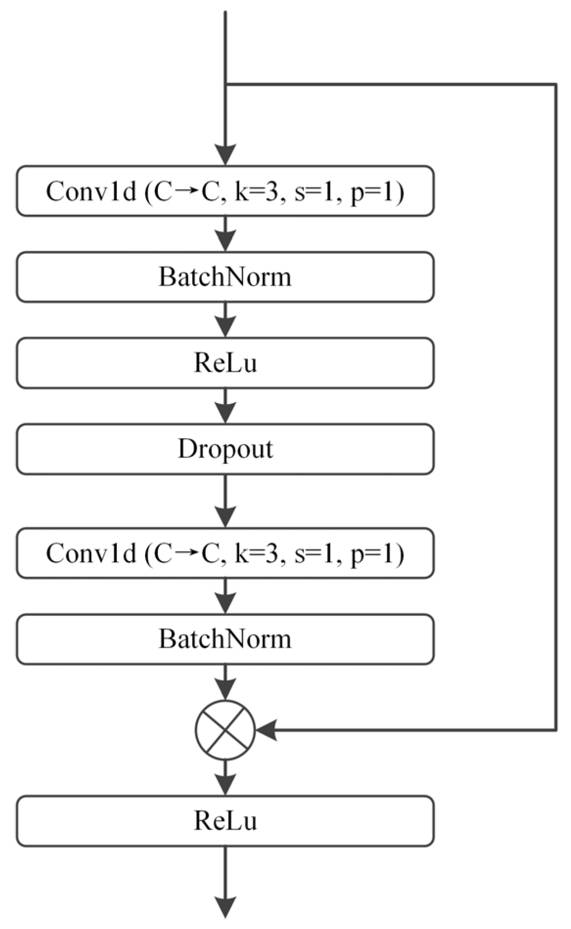
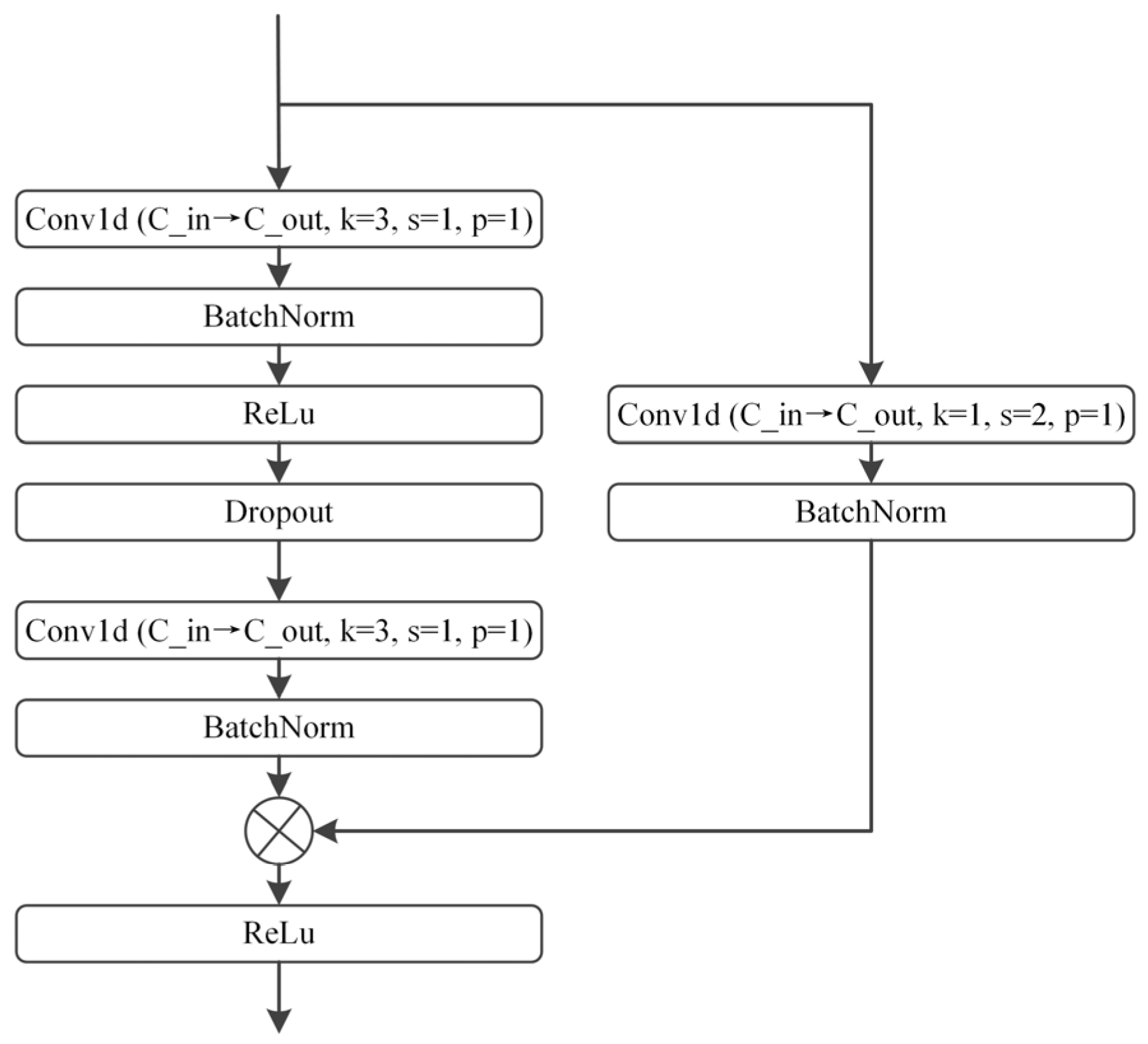
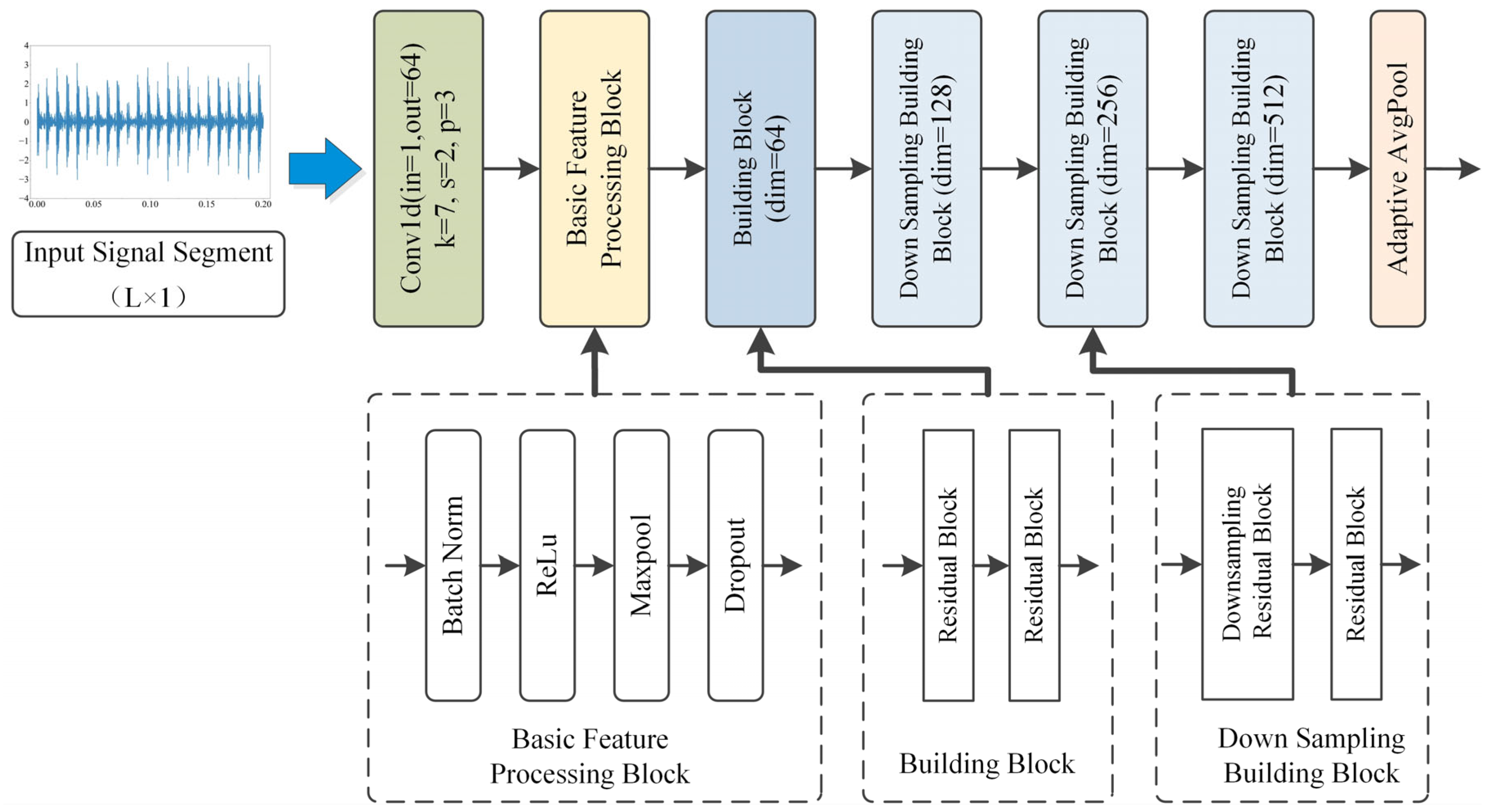
ResNet18 [38] is adapted to construct a 1D-ResNet model specifically designed for one-dimensional signal processing. As shown in Figure 2, the architecture begins with a 1D convolutional layer (kernel size: 7, stride: 2) as the input stem, followed by a feature processing block. The 1D-ResNet comprises four stages of residual building blocks, each consisting of two residual blocks. Each residual block contains two 1D convolutional layers and a skip connection and is categorized as either basic or downsampling based on whether the input and output dimensions match, as illustrated in Figure 3 and Figure 4.

Figure 2. Schematic of the 1D-ResNet branch within the PHDN.

Figure 3. Basic Residual Block.

Figure 4. Downsampling Residual Block.

In the first stage, two consecutive 64-channel basic residual blocks are applied to strengthen initial feature extraction. In each of the subsequent three stages, one downsampling residual block is followed by one basic residual block, progressively increasing the channel count from 64 to 512. Finally, Adaptive Average Pooling layer generates a fixed 512-dimensional feature vector for downstream classification.

2.3. Feature Fusion and Fault Classification

As illustrated in Figure 5, the PHDN model integrates two complementary branches: ConvNeXt for processing time–frequency images and 1D-ResNet for analyzing raw mechanical vibration signals. These dual modalities are processed in parallel to exploit both temporal and spectral characteristics. Specifically, the 512-dimensional feature vector from the 1D-ResNet branch and the 768-dimensional feature vector from the CWT-ConvNeXt branch are concatenated, forming a unified 1280-dimensional fused representation—the PHDN vector.

Figure 5. Architecture of the PHDN model.

The classification module consists of a three-layer feedforward neural network designed to perform hierarchical dimensionality reduction and nonlinear transformation. In the first layer, the concatenated features are projected into a 512-dimensional space, where BatchNorm, ReLU activation, and Dropout are applied to stabilize training, enhance discriminative learning, and improve generalization. The second layer further compresses the representation to 256 dimensions, with BatchNorm and Dropout promoting robust feature interaction and mitigating overfitting. Finally, the third layer maps the learned features into the output space corresponding to fault categories and produces probability predictions via a softmax function.

3. Proposed Methodology

3.1. Vibration Signal Segmentation

In mechanical fault diagnosis, each signal segment must capture all key characteristics of a complete fault cycle. For rolling bearings, common faults such as inner and outer race defects generate periodic impact signals that are synchronized with the bearing’s fundamental frequency. The minimum length of a vibration signal segment is determined by both the rotational speed and the sampling rate, and it is crucial that each segment contains at least one full fault cycle to preserve diagnostic integrity. This minimum length is defined as follows:

$$L_{\min }={\displaystyle \frac{f_s}{f_r}}$$

(1)

where f_s denotes the sampling frequency (in Hz), and f_r represents the fundamental rotational frequency of the bearing (in Hz), calculated as n/60, with n being the equipment’s rotational speed in revolutions per minute (r/min).

To assess the consistency between different segments, the Pearson correlation coefficient is computed between any two signal segments S_i(t) and S_j(t):

$$r={\displaystyle \frac{{\displaystyle \sum \begin{array}{c}L\\ t=1\end{array}\left(S_i(t)-{\mu }_{S_i}\right)\left(S_j(t)-{\mu }_{S_j}\right)}}{\sqrt{{\displaystyle \sum \begin{array}{c}L\\ t=1\end{array}{\left(S_i(t)-{\mu }_{S_i}\right)}^2}}\bullet \sqrt{{\displaystyle \sum \begin{array}{c}L\\ t=1\end{array}{\left(S_j(t)-{\mu }_{S_j}\right)}^2}}}}$$

(2)

where ${\mu }_{S_i}$ and ${\mu }_{S_j}$ are the means of the segments S_i(t) and S_j(t) respectively. A correlation coefficient r close to 1 indicates high similarity, reflecting strong repeatability in fault patterns across segments.

The original vibration signal is partitioned into non-overlapping segments using a fixed window length L. Segments shorter than L are discarded to avoid incomplete representations. Within the interval [L_min, L_max], the average correlation among segments is evaluated to identify the optimal segmentation length that maximizes temporal coherence. To balance feature completeness and sufficient sample size, L_min ensures coverage of at least one full fault cycle, while L_max considers computational efficiency and noise sensitivity. The search range for L is set to (1.2–2.5)·L_min, with candidate lengths evaluated at intervals of 0.1 L_min. This strategy prevents information loss from short segments while avoiding excessive data redundancy from overly long segments.

3.2. Continuous Wavelet Transform (CWT)

The Continuous Wavelet Transform (CWT) is a powerful time–frequency analysis tool that decomposes a signal into scaled and translated versions of a wavelet, enabling detailed characterization of transient features. Mathematically, the CWT is defined as [39]:

$$CW{T}_x(a,b)={\displaystyle \frac{1}{\sqrt{a}}}{\displaystyle {\int }_{-\infty }^{\infty }x\left(t\right)}{\psi }^{\ast }\left({\displaystyle \frac{t-b}{a}}\right)dt$$

(3)

where x(t) is the input signal, a > 0 is the scale parameter, b ∈ ℝ is the translation parameter, ψ is the wavelet function, and * denotes complex conjugation. The key aspect of the continuous wavelet transform (CWT) resides in the selection of an appropriate wavelet function. Generalized Morse wavelets constitute a family of exactly analytic wavelets. They are useful for analyzing modulated signals, which are signals with time-varying amplitude and frequency. The frequency-domain representation of the Morse wavelet is given by [40]

$${\psi }_{\beta ,\gamma }(\omega )=U\left(\omega \right){\alpha }_{\beta ,\gamma }{\omega }^{\beta }{e}^{-{\omega }^{\gamma }}$$

(4)

where α_β,γ is a normalization constant, U(ω) is the unit step function, and β and γ are two parameters controlling the wavelet form. The parameter γ determines the symmetry of the Morse wavelet, while P² = βγ defines the time-bandwidth product. By adjusting the time-bandwidth product and symmetry parameters of a Morse wavelet, it is possible to generate analytic wavelets with diverse characteristics and dynamic behaviors. This inherent customizability enables the method to operate without reliance on fixed waveform templates, allowing for flexible adaptation to the features of non-stationary signals such as mechanical vibrations. It can accurately extract transient components and effectively suppress noise interference, thus serving as a powerful and efficient tool for the analysis of complex time-varying signals. In this study, the complex Morse wavelet was selected as the basis function for the wavelet transform, with the specific parameter settings of γ = 3 and the time—bandwidth product P² = 60.

3.3. Transfer Learning Strategies

Convolutional neural networks (CNNs) have become essential tools in signal processing due to their success in image analysis. However, training CNNs from scratch demands extensive computational resources and long training times. Transfer learning addresses these challenges by initializing the network with pre-trained weights, allowing knowledge transfer from large-scale source datasets to target tasks with limited data. This approach significantly accelerates convergence and improves model generalization.

For PHDN, transfer learning is applied exclusively to the ConvNeXt branch, where weights are initialized from a ConvNeXt-T model pre-trained on ImageNet. As illustrated in Figure 1, the lower layers of ConvNeXt are frozen to retain their ability to extract generic spatial features. Only the higher-level layers are fine-tuned to adapt to the specific texture and pattern characteristics of time–frequency maps derived from mechanical vibration signals. In contrast, the 1D-ResNet branch—designed for one-dimensional raw signals and lacking an equivalent pre-trained counterpart—is trained from scratch to learn temporal fault dynamics effectively. This asymmetric training strategy promotes diverse feature representations across branches while accelerating overall convergence. This scheme is specifically designed as a feasible solution for scenarios with limited hardware resources: it avoids the high computational cost of training both branches from scratch or customizing pre-trained models for 1D signals, while still achieving effective performance.

3.4. Fault Diagnosis Process

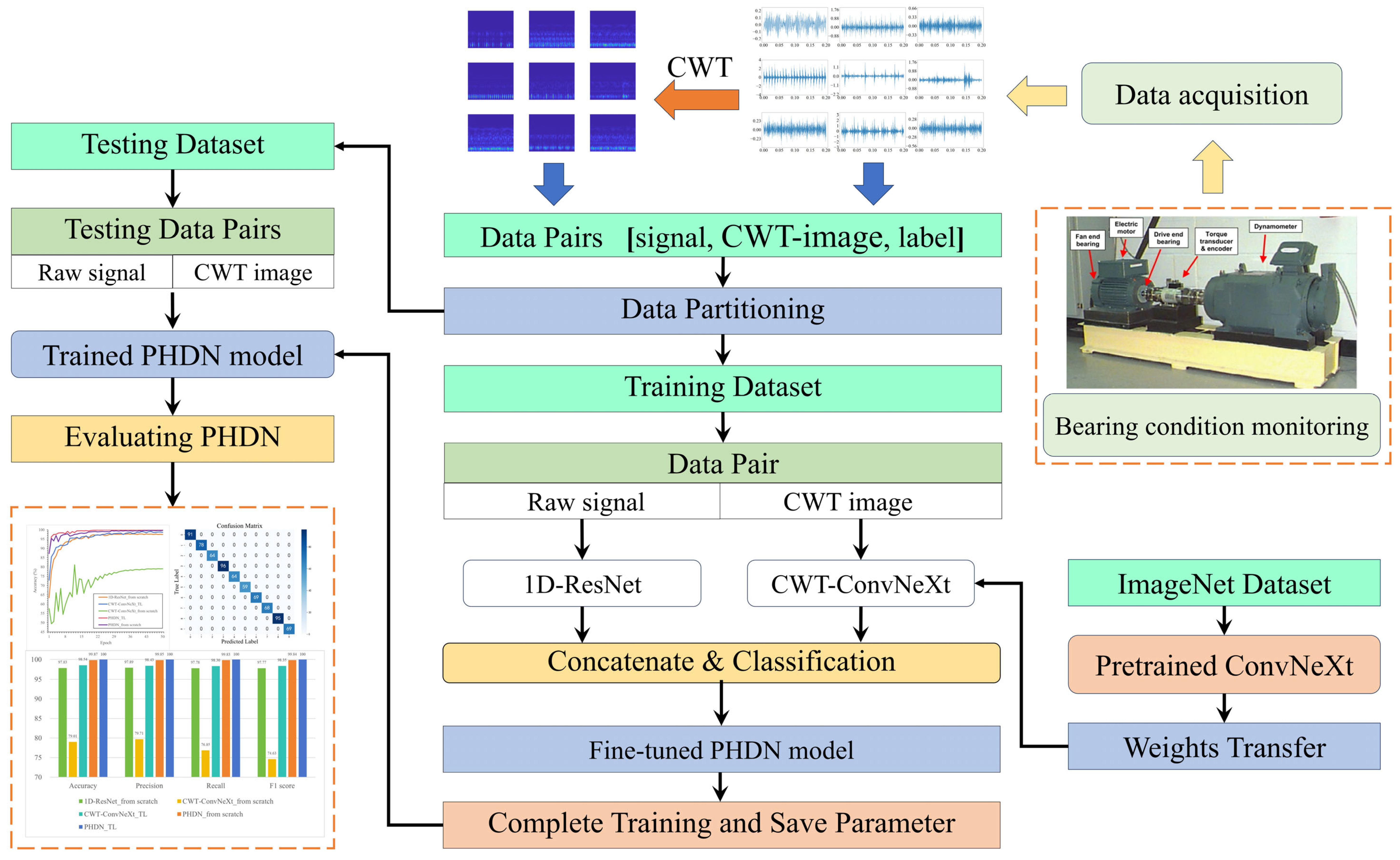
The proposed methodology integrates continuous wavelet transform (CWT), a parallel heterogeneous deep network (PHDN), and transfer learning (TL) to achieve high-precision fault recognition in rotating machinery. The overall workflow is illustrated in Figure 6 and consists of the following steps:

Figure 6. The workflow of the proposed fault diagnosis method.

Data Acquisition: Publicly available bearing datasets are used in this study, consisting of one-dimensional vibration signals collected via sensors. In practical deployment, similar sensors should be installed on machinery to enable real-time data acquisition.

Time–Frequency Image Generation: Since the ConvNeXt branch processes three-channel 2D images, the raw vibration signals are first segmented. Each segment is then transformed into a time–frequency image using continuous wavelet transform (CWT).

Data Pair Construction and Partitioning: Given the dual-input nature of the PHDN, hybrid data pairs are constructed by associating signal segments, their corresponding time–frequency images, and class labels. In each pair, the signal segment is fed into the 1D-ResNet branch, the image into the ConvNeXt branch, and the output is supervised by the label. These pairs are randomly divided into training, validation, and test sets to ensure unbiased evaluation.

Pre-trained Model Initialization: In the ConvNeXt branch, pre-trained weights from the ConvNeXt-T model (loaded via the timm library) are adopted. The input layer and the first two stages of ConvNeXt blocks are frozen to preserve learned low-level image features. The remaining ConvNeXt blocks, along with the entire 1D-ResNet branch and the classification module, are initialized using the default initialization scheme in timm. This setup ensures a stable starting point for joint fine-tuning.

Model Training: The network is trained on the training set until convergence, monitored using the validation set. Upon convergence, all model parameters are saved for inference.

Performance Evaluation: The trained model is evaluated on the test set to assess its accuracy, robustness, and generalization performance in fault diagnosis tasks.

4. Experiment and Result Analysis

To evaluate the generality and effectiveness of the proposed method, this study conducts experiments on two distinct benchmark datasets. The evaluations are performed using the Case Western Reserve University (CWRU) rolling bearing dataset [41] and the vibration subset of the multimodal rotating machinery dataset under variable operating conditions released by the Korean Academy of Science and Technology (KAIST) [42]. All models are implemented in PyTorch 2.5.1 with CUDA 12.4 support, running on a workstation equipped with an Intel i7-114650HX processor and an NVIDIA RTX 4070 Ti graphics card. The model training hyperparameters were determined through a combination of literature review and preliminary experimental tuning to ensure both rationality and effectiveness. Based on parameter configurations reported in relevant studies [43], we initially set the learning rate to 0.0001 and employed the AdamW optimizer to minimize the cross-entropy loss function, with a weight decay coefficient of 5 × 10⁻⁵. For batch size selection, comparative experiments were conducted on the CWRU dataset using candidate values of 32, 64, and 128. Although a batch size of 128 yielded the highest training accuracy, followed by 32, we ultimately chose 32 to achieve an optimal balance between model performance and hardware resource limitations. The model was trained for a total of 50 epochs to ensure sufficient convergence. To enhance training stability and convergence behavior, a cosine annealing learning rate schedule is applied. Performance is evaluated using standard classification metrics: accuracy (ACC), precision (P), recall (R), F1 score, and specificity.

$$ACC={\displaystyle \frac{TP+TN}{TP+TN+FP+FN}}$$

(5)

$$P={\displaystyle \frac{TP}{TP+FP}}$$

(6)

$$R={\displaystyle \frac{TP}{TP+FN}}$$

(7)

$$F1={\displaystyle \frac{2\times \left(P\times R\right)}{P+R}}$$

(8)

$$Specificity={\displaystyle \frac{TN}{TN+FP}}$$

(9)

where TP denotes the number of true positive cases, FP denotes the number of false positive cases, and TN and FN denote the number of true negative and false negative cases, respectively.

4.1. Experimental Validation on the CWRU Dataset

4.1.1. Data Description

The CWRU bearing fault dataset was selected to evaluate model performance. As illustrated in Figure 7, the test rig comprises a 2 hp three-phase induction motor, a torque transducer, and a dynamometer. Single-point faults were artificially introduced on the surfaces of SKF deep groove ball bearings using electrical discharge machining (EDM). Defects with diameters of 0.007 in (0.1778 mm), 0.014 in (0.3556 mm), and 0.021 in (0.5334 mm) were created on the rolling elements, inner race, and outer race, respectively. Vibration acceleration signals were collected from both the drive-end and fan-end bearings. Thus, each load condition includes nine distinct fault types, corresponding to three severity levels and three fault locations. In this work, fault data under a load level of 0 hp and a rotational speed of 1797 rpm were used to assess model performance, with a sampling frequency of 12.5 kHz. Including the normal operating condition, the fault diagnosis task is formulated as a 10-class classification problem, as summarized in Table 1. The vibration signals were converted into 224 × 224-pixel RGB time–frequency images using continuous wavelet transform (CWT), and hybrid data pairs were constructed accordingly. The dataset was then divided into training, validation, and test sets in a 7:1.5:1.5 ratio.

Figure 7. CWRU bearing test rig [41].

Table 1. Description of the rolling bearing fault dataset.

Class Label	Fault Location	Fault Size	Segment Length
0	Normal	-	802
1	Inner Race	0.007″	642
2	Ball	0.007″	1003
3	Outer Race	0.007″	561
4	Inner Race	0.014″	962
5	Ball	0.014″	1003
6	Outer Race	0.014″	802
7	Inner Race	0.021″	882
8	Ball	0.021″	962
9	Outer Race	0.021″	802

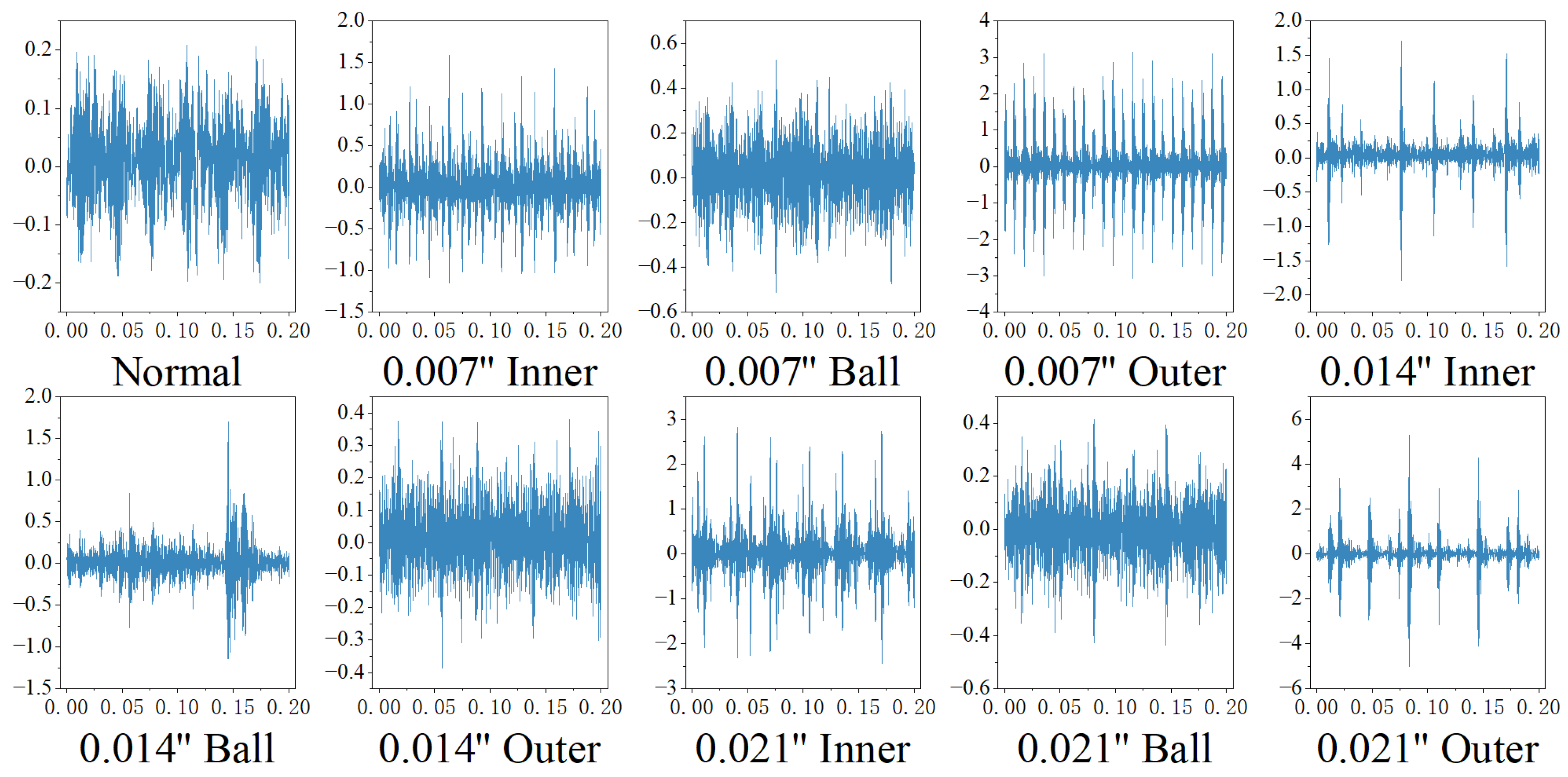
Figure 8 presents the original vibration signals for each of the 10 fault categories. The minimum signal length L_min for the bearing is calculated according to Equation 1, and the optimal window size is determined by analyzing the correlation among signal segments within the range of 1.2 to 2.5 times L_min. The segment lengths of the signals across the 10 operating states are detailed in Table 1. The segmented vibration signal portions are converted into two-dimensional time–frequency images using the continuous wavelet transform (CWT) as illustrated in Figure 9.

Figure 8. Raw vibration signal of the CWRU dataset.

Figure 9. CWT Time–frequency representation of the CWRU dataset.

4.1.2. Experimental Results and Analysis

(1)

Verification of Transfer Learning Strategy

To validate the effectiveness of the transfer learning strategy and demonstrate that the diagnostic performance of the PHDN model is superior to that of standalone models, comparative experiments were conducted between models with pre-trained weights and those trained from scratch. The evaluated models include CWT-ConvNeXt, 1D-ResNet, and PHDN. Among them, 1D-ResNet employs the classification block proposed in this paper and was trained entirely from scratch. For CWT-ConvNeXt and the PHDN model, the ConvNeXt backbone and its pre-trained parameters were obtained via the timm library’s application module to facilitate model transfer.

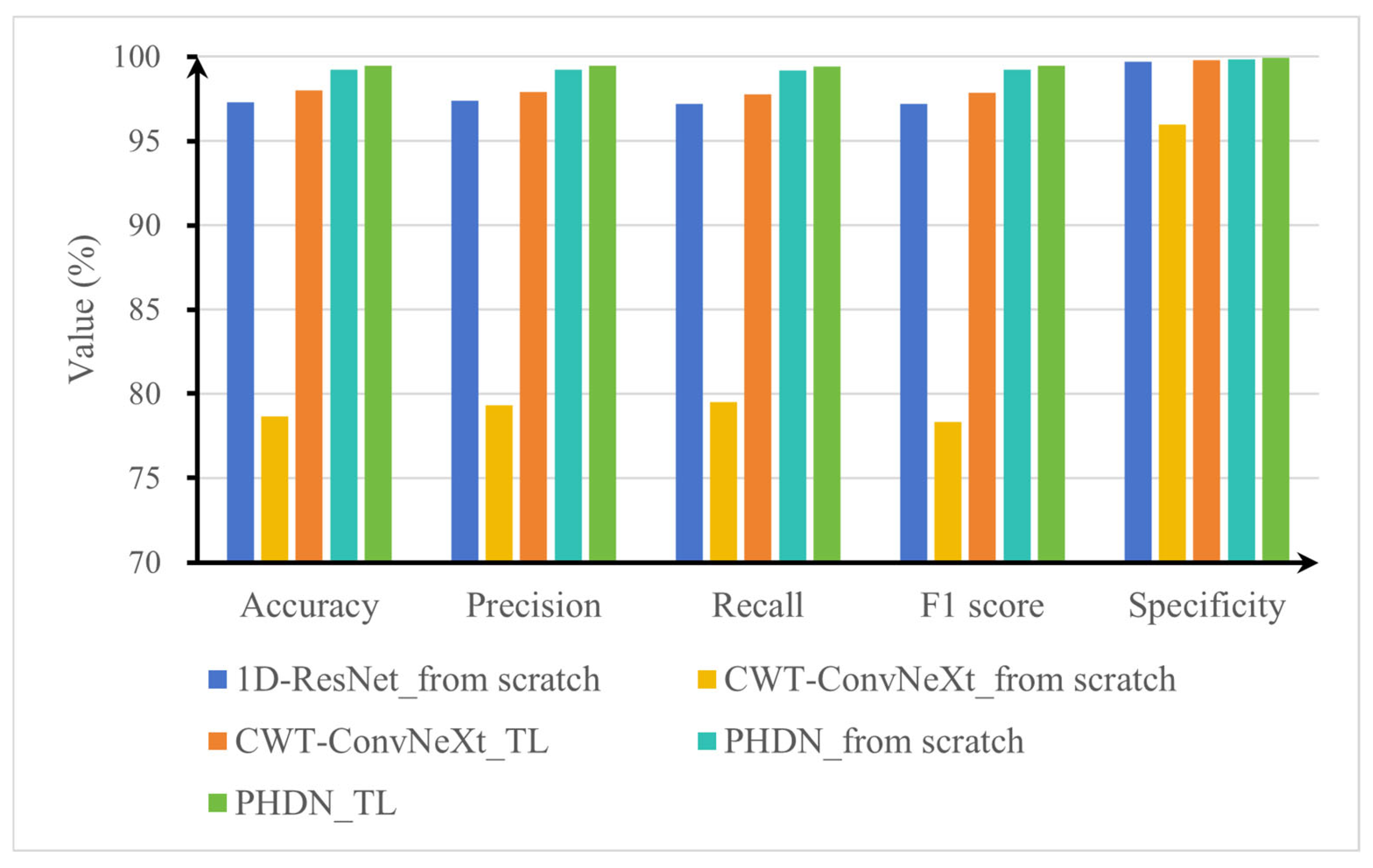
Each test was independently conducted five times. The results reported in Table 2 present the mean and standard deviation across these repetitions, and the average processing time per epoch for each model was also recorded. Figure 10 displays the test results for the five networks. Clearly, CWT-ConvNeXt without pre-trained parameters achieves only 79.01% accuracy. However, when parameter transfer is applied, the accuracy improves significantly to 98.54%. 1D-ResNet performs robustly, achieving 97.83% accuracy when trained from scratch. The PHDN model reaches 99.87% accuracy when trained from scratch and achieves perfect 100% accuracy after incorporating pre-trained parameters. Similar trends are observed in recall, precision, and F1 score, all of which support the conclusion that the transfer learning strategy is effective, and that the hybrid architecture of PHDN enhances fault recognition accuracy. Table 2 presents the detailed experimental results and the average training time per epoch.

Table 2. Identification results of the model.

Model	Accuracy	Precision	Recall	F1 Score	Specificity	Training Time
1D-ResNet_from scratch	97.31% ± 0.78	97.37% ± 0.77	97.22% ± 0.78	97.21% ± 0.76	99.69% ± 0.20	21.14 s ± 0.55
CWT-ConvNeXt_TL	98.02% ± 0.29	97.91% ± 0.28	97.78% ± 0.27	97.84% ± 0.27	99.78% ± 0.11	23.52 s ± 0.18
CWT-ConvNeXt_from scratch	78.64% ± 0.66	79.33% ± 0.67	79.50% ± 0.68	78.32% ± 0.67	95.99% ± 0.28	23.45 s ± 0.21
PHDN_TL	99.47% ± 0.34	99.48% ± 0.33	99.43% ± 0.38	99.45% ± 0.36	99.94% ± 0.04	35.50 s ± 0.24
PHDN_from scratch	99.24% ± 0.41	99.22% ± 0.42	99.20% ± 0.42	99.21% ± 0.43	99.83% ± 0.07	35.68 s ± 0.32

Figure 10. Test results comparison between models trained from scratch and those using TL strategy.

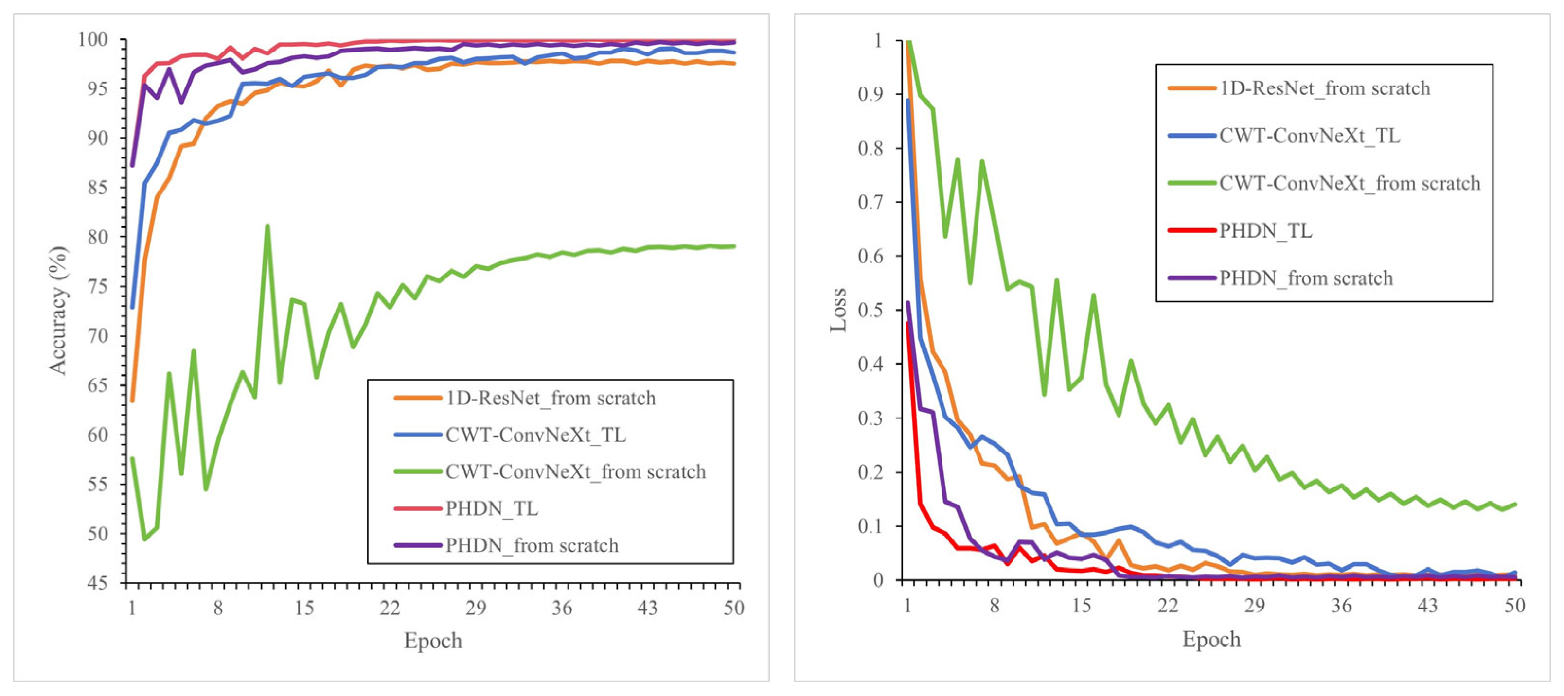
Figure 11 illustrates the increase in accuracy and the corresponding reduction in loss across training epochs for each model. At the end of training, CWT-ConvNeXt trained from scratch achieves an accuracy below 80%, while 1D-ResNet exceeds 97% and CWT-ConvNeXt with pre-trained parameter transfer surpasses 98%. The PHDN model achieves over 99% accuracy regardless of whether transfer learning is applied, with a marginal improvement observed when pre-trained parameters are utilized. Furthermore, PHDN demonstrates consistently higher accuracy than standalone models during most stages of training, and its loss curve reaches a flat phase after 20 training epochs and converges to one of the lowest values, indicating strong optimization performance. Therefore, during all the following experiments, the pre-trained transfer learning strategy will be employed.

Figure 11. Accuracy and loss curves of each model during training.

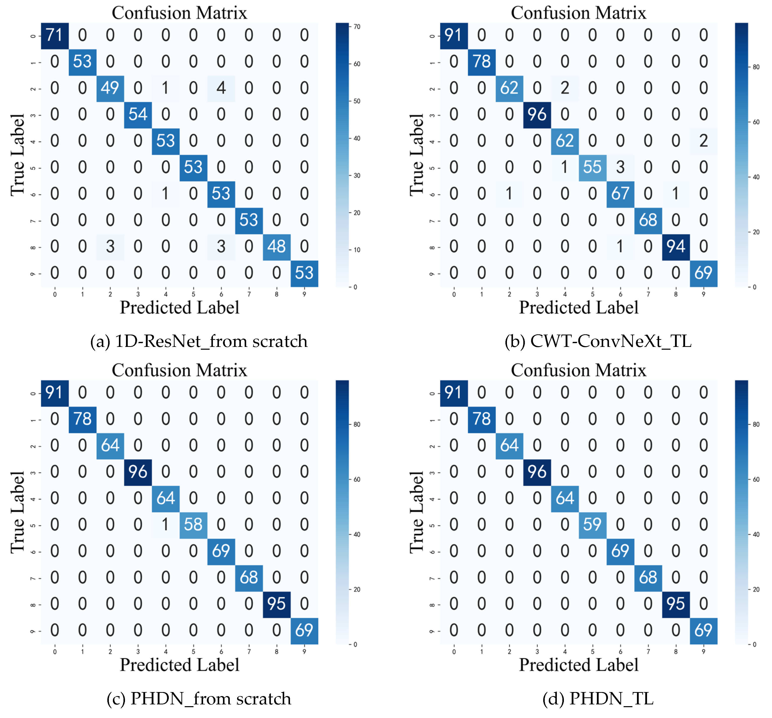
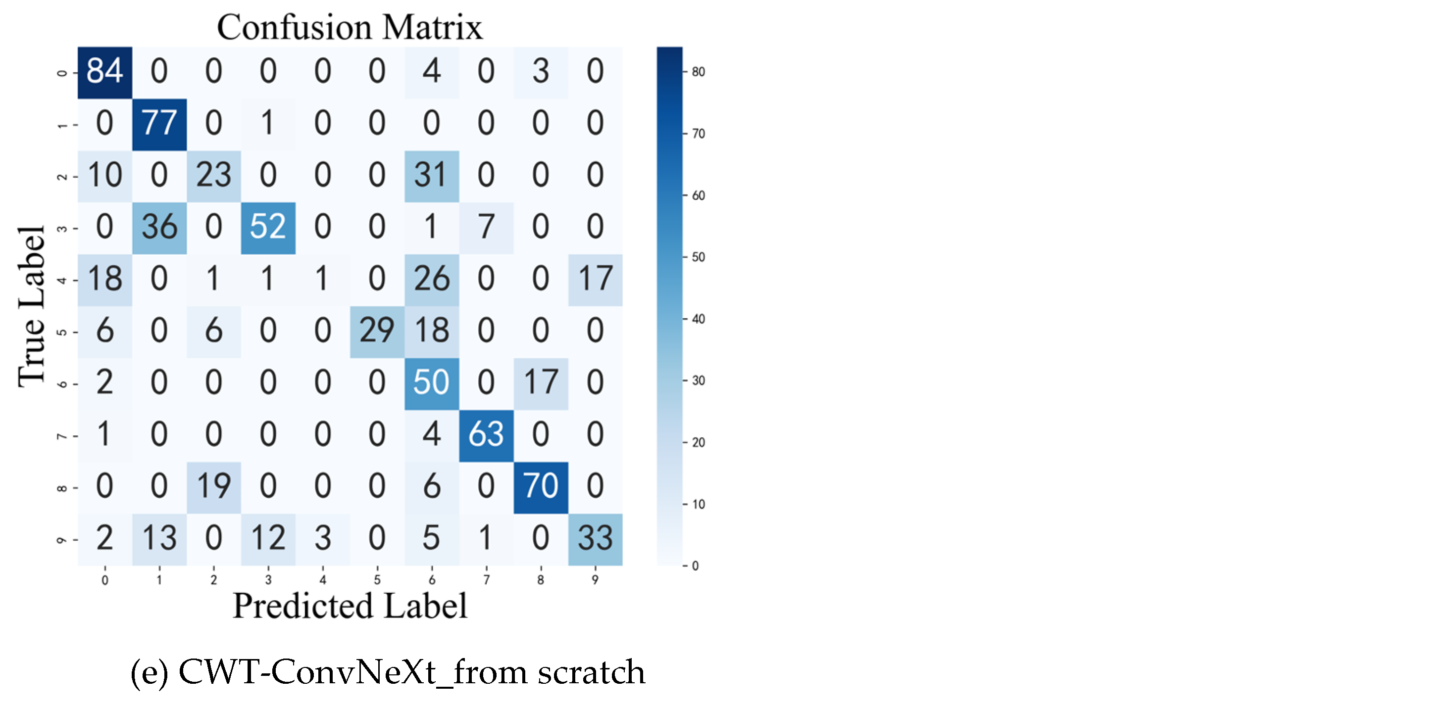
To further analyze the classification performance of each method, confusion matrices are provided to visualize the detailed test results. Figure 12 shows the confusion matrices for the standalone models and the PHDN model. In these matrices, the horizontal axis represents predicted labels, while the vertical axis indicates true labels.

Figure 12. Confusion matrices.

(2)

Fault Diagnosis under Different Noise Intensities

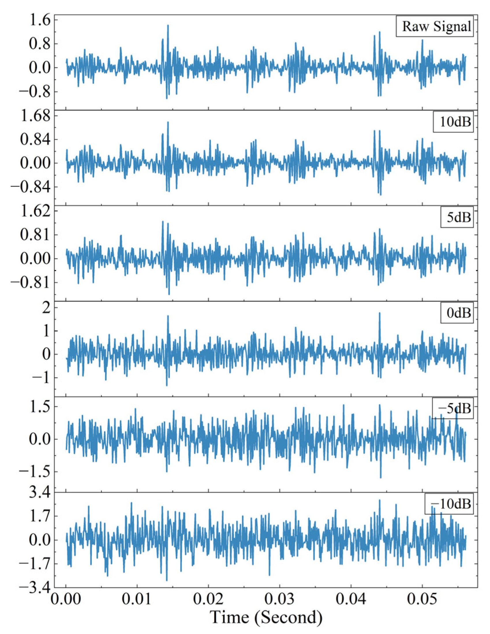
Due to the widespread nature of mechanical equipment vibrations, the collected rolling bearing data are often contaminated by noise. It is essential to evaluate whether the proposed model can achieve accurate diagnosis under noisy conditions. To simulate realistic environmental interference, Gaussian noise was added to the raw signals, generating test datasets with varying signal-to-noise ratios (SNR). The time-domain waveforms of these signals at different SNR levels are shown in Figure 13, with SNR values set to 10 dB, 5 dB, 0 dB, −5 dB, and −10 dB. By conducting experiments across various noise intensities, the stability and adaptability of PHDN in practical applications can be comprehensively assessed, demonstrating the performance enhancement enabled by cross-modal fusion. For each test, five independent repetitions were performed, with the mean value and standard deviation of these replicates summarized in Table 3.

Figure 13. Time-domain signal waveforms for different signal-to-noise ratios.

Table 3. The results of diagnostic accuracy (%) under different SNRs.

Model	SNR (dB)
	−10	−5	0	5	10
1D-ResNet	63.16 ± 4.71	78.39 ± 2.94	89.80 ± 1.86	94.83 ± 1.63	96.81 ± 1.44
CWT-ConvNeXt	78.69 ± 2.17	88.30 ± 1.46	93.75 ± 1.10	97.48 ± 1.02	98.07 ± 0.93
PHDN	86.23 ± 1.39	91.21 ± 1.14	98.18 ± 0.92	98.31 ± 0.68	99.80 ± 0.06

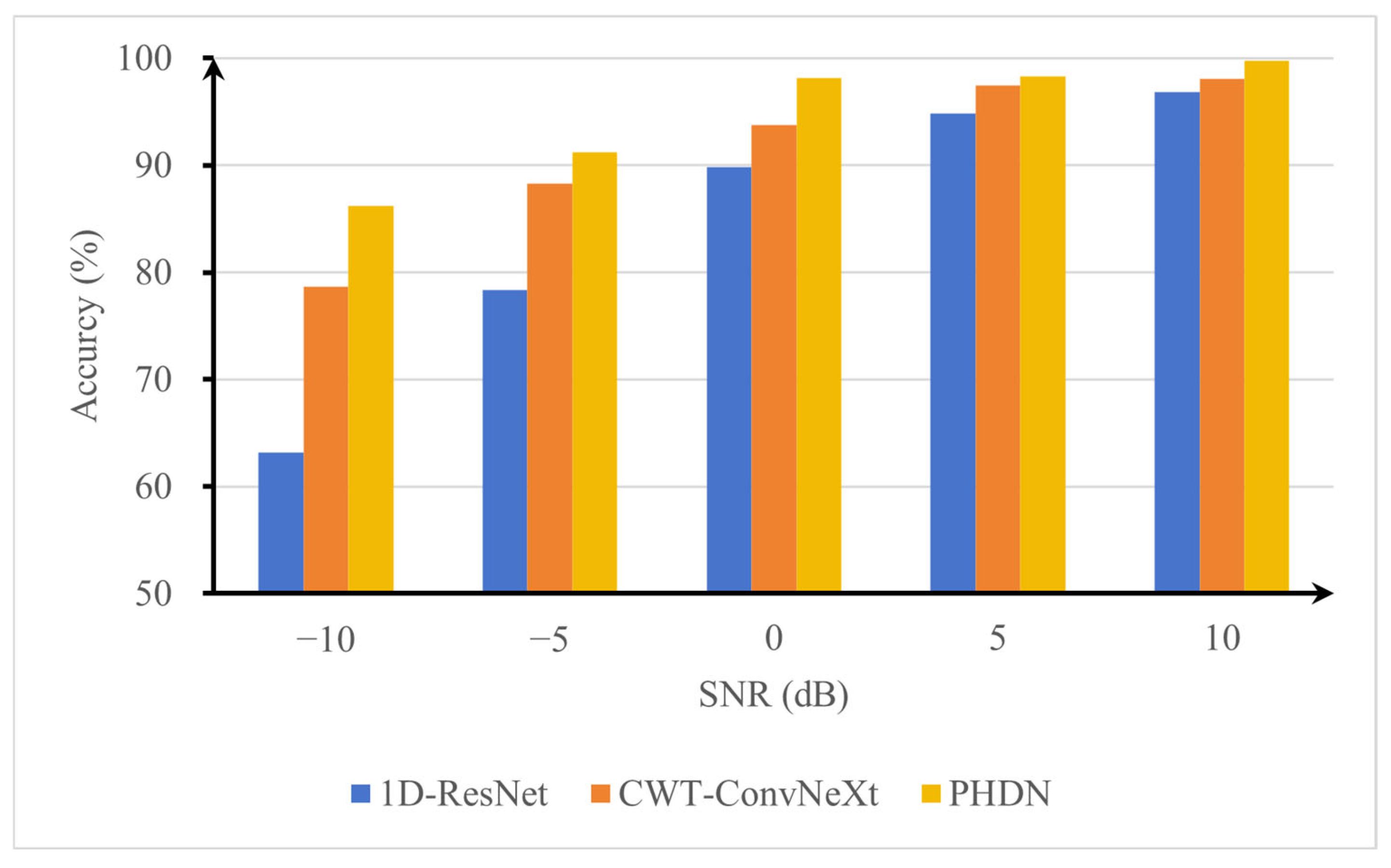
Figure 14 presents the recognition accuracy of PHDN under varying signal-to-noise ratio (SNR) conditions. As the SNR decreases from 10 dB to −10 dB, noise intensity progressively increases. At 10 dB, the accuracy reaches 99.80%, slightly higher than the 98.31% observed at 5 dB. This is because the lower noise level allows for better preservation of fault features, facilitating more discriminative feature extraction. In contrast, the moderate interference at 5 dB introduces minor signal distortions, resulting in a marginal decline in model performance. Both the standalone model and PHDN achieve high diagnostic accuracy at 10 dB and 5 dB, demonstrating strong robustness in low-noise environments. When the SNR drops to 0 dB, the standalone model exhibits a significant performance degradation, whereas PHDN maintains relatively stable accuracy, reflecting its enhanced stability. As noise intensifies further below 0 dB, indicating that noise power exceeds signal power, fault pulses are severely obscured, leading to a notable decline in recognition performance across all models. At −5 dB, as illustrated in Figure 13, the original signal waveform becomes nearly indistinguishable, with vibration characteristics completely overwhelmed by noise; nevertheless, PHDN sustains an accuracy above 90% (12.82% higher than 1D-ResNet and 2.91% higher than CWT-ConvNeXt), highlighting its resilience under moderate noise conditions. However, when the SNR further declines to −10 dB, PHDN’s accuracy drops markedly to 86.23%, yet it still outperforms the two standalone models.

Figure 14. Diagnostic accuracy under different signal-to-noise ratios.

(3)

Fault Diagnosis under Insufficient Training Samples

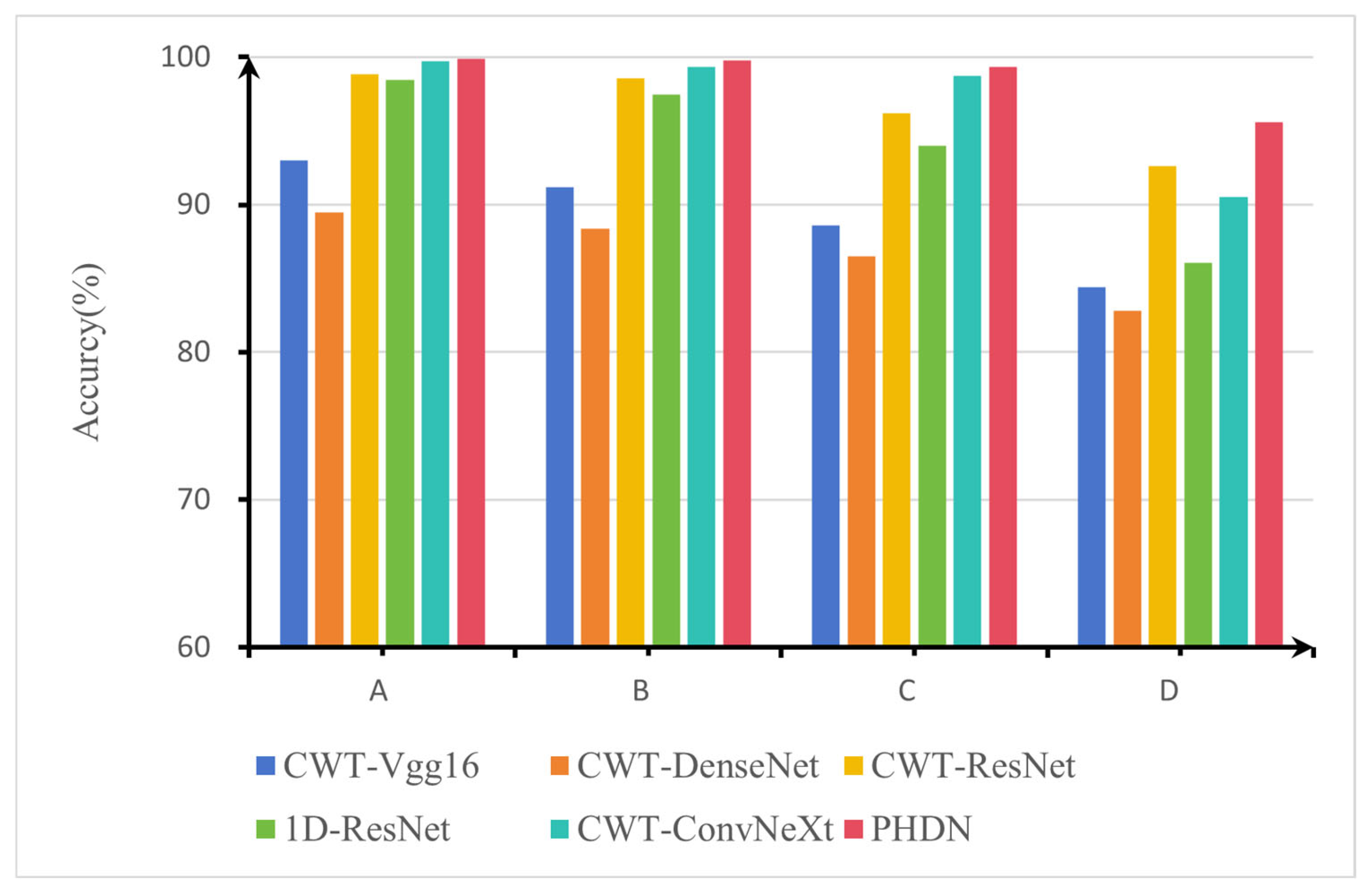
Bearing data collection is often constrained by operational conditions, making it difficult to acquire sufficient labeled samples for model training. Therefore, evaluating the fault diagnosis performance of PHDN under limited data conditions is essential. Building upon the prior experimental setup, four datasets—labeled A, B, C, and D—were constructed by selecting 100%, 50%, 30%, and 15% of the original training data, respectively. The validation and test sets remained unchanged across all experiments to ensure consistency. In addition to comparing PHDN with 1D-ResNet and CWT-ConvNeXt, we included three widely used deep learning architectures—VGG16, DenseNet201, and ResNet18—for benchmarking. All three were implemented using pre-trained weights with transfer learning for the purpose of comparison. To improve statistical reliability, each configuration was evaluated 10 independent trials, and the average diagnostic accuracy and standard deviation was reported in Table 4 as the final result.

Table 4. The results of diagnostic accuracy (%) different sample sizes.

Model	Sample Size
	A (100%)	B (50%)	C (30%)	D (15%)
CWT-Vgg16	93.03 ± 1.12	91.21 ± 1.82	88.57 ± 4.42	84.41 ± 5.61
CWT-DenseNet	89.45 ± 1.08	88.38 ± 1.60	86.51 ± 2.94	82.83 ± 4.68
CWT-ResNet	98.85 ± 0.26	98.59 ± 0.41	96.21 ± 2.75	92.62 ± 4.22
1D-ResNet	98.47 ± 0.90	97.44 ± 1.03	93.97 ± 4.55	86.04 ± 7.35
CWT-ConvNeXt	99.70 ± 0.22	99.32 ± 0.39	98.71 ± 0.94	90.53 ± 3.18
PHDN	99.89 ± 0.08	99.77 ± 0.14	99.35 ± 0.51	95.62 ± 1.21

Figure 15 and Table 4 present the diagnostic accuracy of all models under varying sample sizes. At 100% and 50% sampling ratios, all methods achieve high accuracy, reflecting their expected performance under adequate training data. When the sample size is reduced to 30%, the accuracy of most models begins to decline at varying rates, whereas PHDN and CWT-ConvNeXt demonstrate greater stability. Under the most challenging condition where only 15% of the training data is available, the diagnostic accuracies of all models drop significantly, whereas PHDN exhibits only a 4% decrease. Across all settings, PHDN achieves the highest average accuracy and maintains performance above 99% on datasets A, B, and C, highlighting its superior robustness and effectiveness in few shot scenarios.

Figure 15. Diagnostic accuracy for different sample sizes.

4.2. Experimental Validation on the KAIST Dataset Under Variable Loads

This section validates the effectiveness of the proposed method under variable load conditions. The experimental data were collected from the bearing test rig at the Korean Academy of Science and Technology. As illustrated in Figure 16, the test rig comprises a motor, gearbox, torque meter, two sets of bearings, mass wheels, and a hysteresis brake. The load was adjusted using the hysteresis brake at three torque levels: 0 Nm, 2 Nm, and 4 Nm, while the rotational speed was kept constant at 3010 r/min. Fault types include inner race, outer race, and ball defects with diameters of 0.3 mm, 1.0 mm, and 3.0 mm, as well as shaft parallel misalignment (0.1–0.5 mm) and rotor unbalance (583–3318 mg). A total of 45 distinct operating conditions were defined. In this study, only the vibration signal channel was used, and for each fault type, the medium severity level was selected. Three datasets were constructed under the three load conditions and labeled as N1, N2, and N3, respectively. Each dataset includes five fault types along with the normal condition, forming a six-class fault diagnosis task, as summarized in Table 5. Specifically, 70% of the samples were randomly assigned to the training set, 15% to the validation set, and the remaining 15% to the test set. The signal segmentation method employed in this case is the same as that in the previous experiment. The diagnostic models used the same hyperparameters as those in the CWRU dataset experiments, except that the number of output classes was adjusted to six.

Figure 16. KAIST bearing test rig [42].

Table 5. Description of the rolling bearing fault dataset under each operational condition.

Class Label	Fault Type	Failure Level	Load	Segment Length	Group
0	Normal	-	0 Nm	1226	N1
			2 Nm	1124	N2
			4 Nm	1124	N3
1	Inner Race	1.0 mm	0 Nm	971	N1
			2 Nm	929	N2
			4 Nm	869	N3
2	Outer Race	1.0 mm	0 Nm	1124	N1
			2 Nm	1175	N2
			4 Nm	1175	N3
3	Ball	1.0 mm	0 Nm	1226	N1
			2 Nm	1278	N2
			4 Nm	1184	N3
4	Misalignment	0.3 mm	0 Nm	1022	N1
			2 Nm	1022	N2
			4 Nm	1022	N3
5	unbalance	1751 mg	0 Nm	869	N1
			2 Nm	869	N2
			4 Nm	767	N3

4.2.1. Fault Diagnosis Under Different Loads

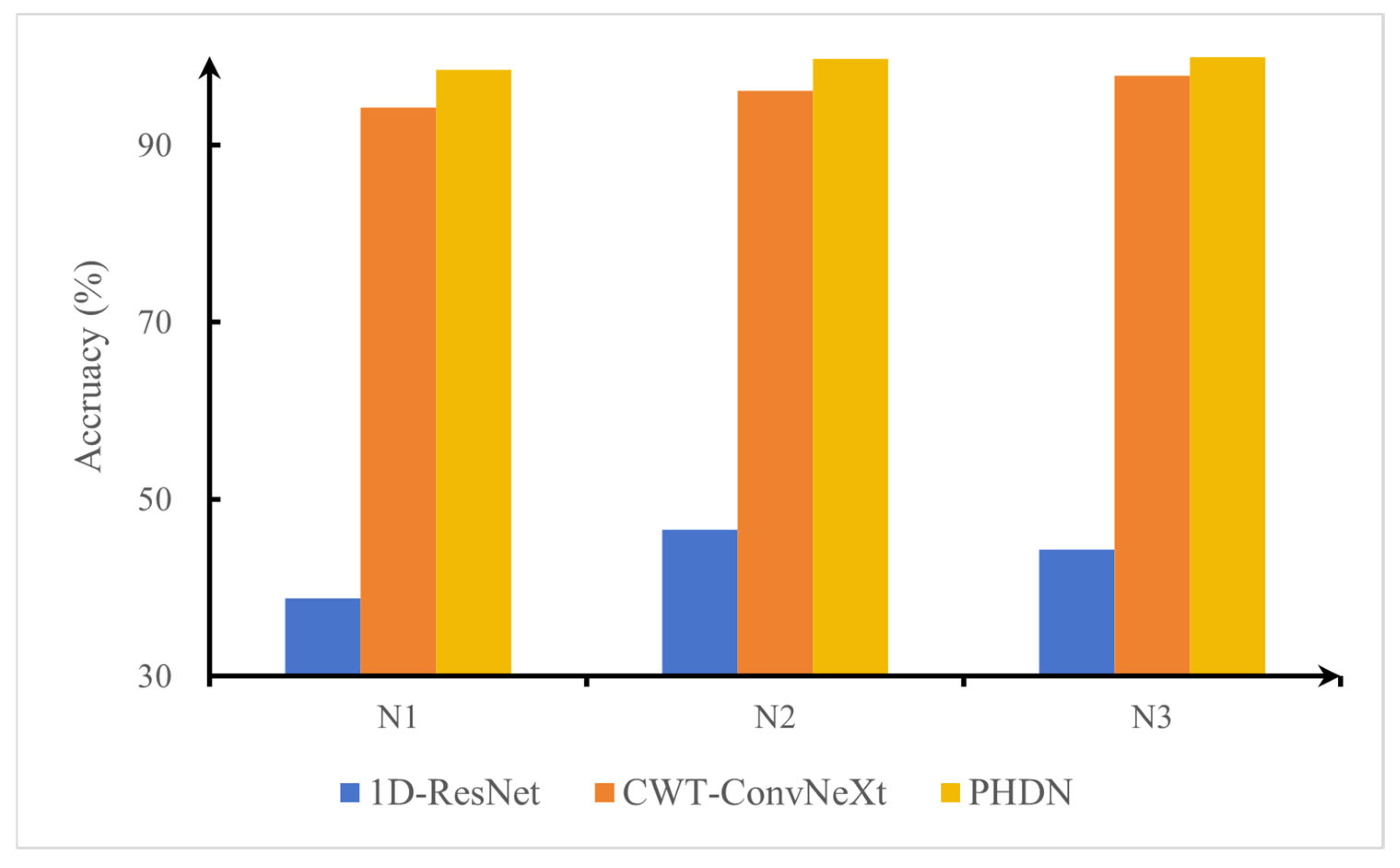
Each set of experiments was independently repeated five times, and the average accuracy and standard deviation were calculated to evaluate model performance across varying operating conditions. The “training time” in Table 6 refers to the average duration required for the model to complete one training epoch under three distinct load conditions. Figure 17 and Table 6 present the recognition results obtained under three different load conditions. PHDN and CWT-ConvNeXt demonstrate superior overall performance, whereas 1D-ResNet achieves accuracies below 50% across all conditions, indicating limited model robustness. Notably, PHDN exhibits high stability and minimal sensitivity to load variations, with accuracies of 98.53%, 99.72%, and 99.87% under N1, N2, and N3 conditions, respectively, reflecting a variation of only approximately 2%. CWT-ConvNeXt also performs well, achieving accuracies of 94.24%, 96.17%, and 97.81% across the three conditions, with a variation of about 4%. Comparative analysis further confirms that PHDN consistently outperforms CWT-ConvNeXt. These results validate the effectiveness of the proposed feature fusion strategy in enhancing standalone model performance and improving fault diagnosis robustness under varying load conditions.

Table 6. The results of diagnostic accuracy under different loads.

Model	N1 (%)	N2 (%)	N3 (%)	Training Time (s)
1D-ResNet	38.83 ± 3.54	46.56 ± 2.61	44.31 ± 2.28	30.72 ± 0.67
CWT-ConvNeXt	94.24 ± 1.09	96.17 ± 0.88	97.81 ± 0.79	39.98 ± 0.15
PHDN	98.53 ± 0.25	99.72 ± 0.22	99.87 ± 0.03	52.98 ± 0.37

Figure 17. Diagnostic accuracy under different loads.

4.2.2. Load Variation Validation

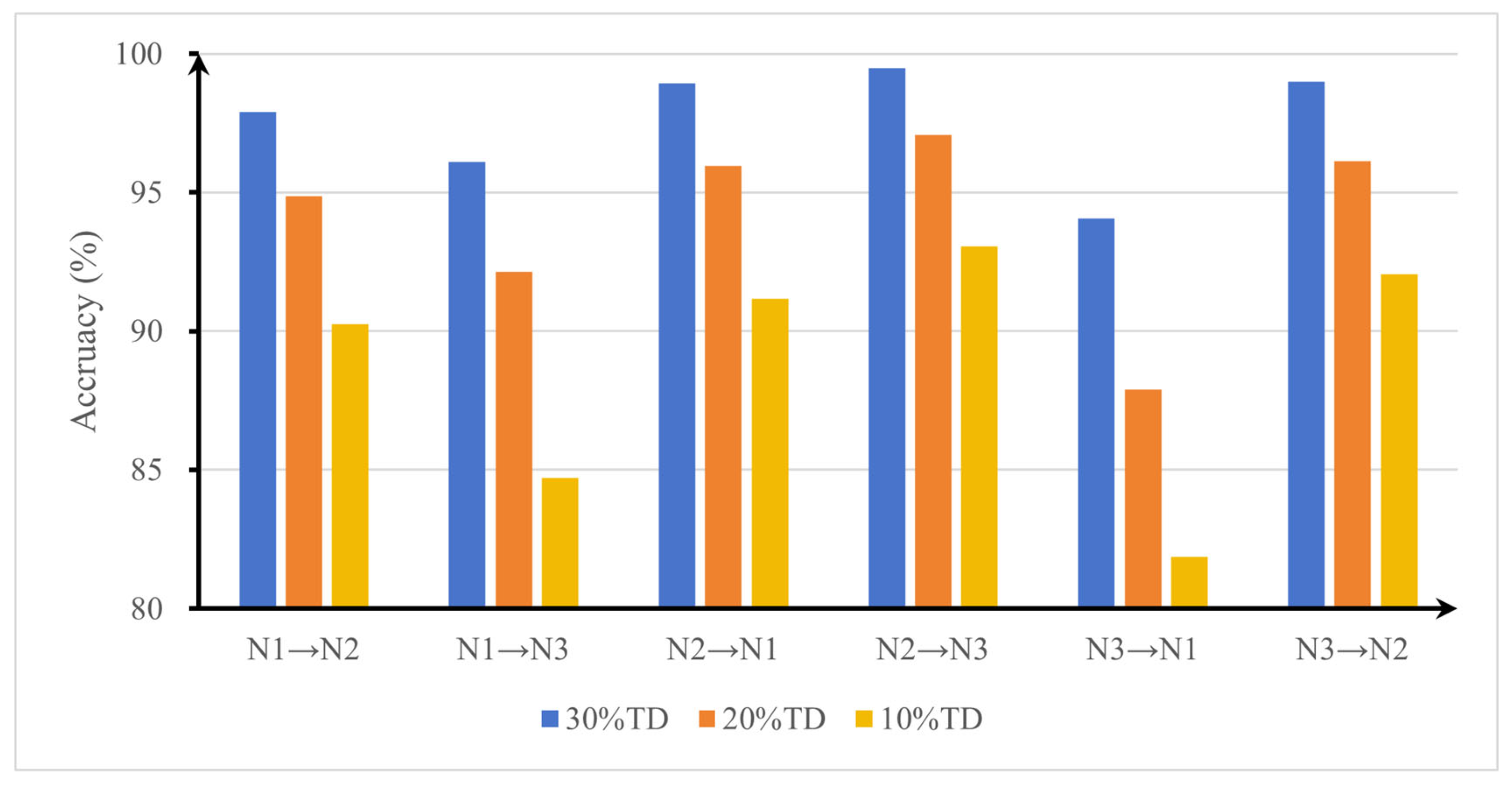
Due to the inherent variability of mechanical equipment and operating conditions, vibration signals are often subject to load variations. Therefore, a model with strong generalization capability is essential. In Figure 18, the notation N1 → N2 indicates that dataset N1 serves as the training set and dataset N2 as the test set. The PHDN model pre-trained on dataset N1 in the prior experiment is directly reused, and 10%, 20%, and 30% of the samples from the target domain (TD) are selected to fine-tune the model, simulating real-world scenarios with limited data availability in the target domain. All other experimental settings remain consistent. Each configuration is evaluated five times, and the average recognition accuracy and standard deviation is reported in Table 7.

Figure 18. Average diagnostic under variable load conditions.

Table 7. The results of diagnostic accuracy (%) under variable load conditions.

Sample Percentage	Transfer Task
	N1 → N2	N1 → N3	N2 → N1	N2 → N3	N3 → N1	N3 → N2
30%TD	97.90 ± 0.51	96.10 ± 0.82	98.95 ± 0.36	99.48 ± 0.26	94.05 ± 1.11	98.98 ± 0.40
20%TD	94.85 ± 1.01	92.15 ± 1.55	95.95 ± 0.91	97.08 ± 0.70	87.90 ± 1.72	96.12 ± 0.84
10%TD	90.25 ± 1.53	84.72 ± 2.08	91.17 ± 1.25	93.05 ± 1.00	81.86 ± 2.26	92.05 ± 1.12

As illustrated in Figure 18, when the sample size reaches 30%, recognition accuracy remains remarkably high, exceeding 95% across all transfer scenarios except N3 → N1, due to the maximum load variation between domains. As the amount of target domain data decreases, test accuracy under different operating conditions exhibits a consistent downward trend. When the sample size is reduced to 10%, the fine-tuned model achieves a minimum test accuracy of 81.86% in the N3 → N1 transfer scenario, followed by 84.72% in the N1 → N3 scenario. This result indicates that the discrepancy in data distribution between the source and target domains significantly impacts the performance of transfer learning. Table 7 summarizes the detailed experimental results.

5. Conclusions

To deal with the challenges of rolling bearing fault diagnosis under complex operating conditions, this paper proposes a parallel heterogeneous deep network (PHDN) to enhance the accuracy and robustness of fault diagnosis. Experimental results demonstrate that the proposed model achieves superior performance on both the CWRU and KAIST datasets. Under varying signal-to-noise ratio (SNR) conditions, the model maintains a recognition accuracy above 90% when SNR is greater than −5 dB. It improves the diagnostic accuracy by 3.8% over the standalone model. In low-sample scenarios using 100%, 50%, 30%, and 15% of the training data, the diagnostic accuracy of the model improves by 3.24% compared to the standalone model under the minimum sample size condition, significantly outperforming the compared methods. Under variable load conditions, PHDN achieves a diagnostic accuracy improvement of at least 2.11 percentage points over the top-performing competitor CWT-ConvNeXt, and successful cross-load model transfer is achieved.

The proposed PHDN effectively enhances fault diagnosis accuracy and robustness through cross-modal feature learning, particularly in challenging environments involving noise interference, limited training samples, and load variations. The key innovation lies in its ability to leverage the complementary strengths of multimodal data via a parallel heterogeneous architecture and cross-modal feature fusion mechanism. This approach not only improves diagnostic accuracy but also strengthens the model’s adaptability and generalization capability under diverse operational conditions, demonstrating significant engineering application potential. Despite these advancements, this study has certain limitations. The model evaluation was conducted exclusively on two laboratory-based benchmark datasets characterized by controlled experimental conditions and isolated fault modes, which may not adequately represent the complexity of real-world industrial environments, including load and speed fluctuations, multi-source noise interference, and the coupled effects of compound faults. Regarding transfer learning approaches, we acknowledge this is not claimed to be the “optimal” approach, but rather a practical, hardware-friendly solution that balances computational efficiency and diagnostic performance. Consequently, the generalizability of the findings to practical industrial applications warrants further validation. Future work will focus on optimizing the network architecture to reduce computational overhead and improve real-time inference performance. Additionally, cross-device and cross-domain transfer learning strategies will be investigated to further validate and enhance the model’s generalization across different systems and environments.

References

1. Liu, D.; Cui, L.; Cheng, W. Flexible Generalized Demodulation for Intelligent Bearing Fault Diagnosis Under Nonstationary Conditions. IEEE Trans. Ind. Inform. 2023, 19, 2717–2728. [Google Scholar] [CrossRef]
2. Jiang, G.; Yang, J.; Cheng, T.; Sun, H. Remaining useful life prediction of rolling bearings based on Bayesian neural network and uncertainty quantification. Qual. Reliab. Eng. Int. 2023, 39, 1756–1774. [Google Scholar] [CrossRef]
3. Raj, K.; Kumar, S.; Kumar, R. Systematic Review of Bearing Component Failure: Strategies for Diagnosis and Prognosis in Rotating Machinery. Arab. J. Sci. Eng. 2025, 50, 5353–5375. [Google Scholar] [CrossRef]
4. Ma, H.; Fan, C.; Zhang, Y.; Wang, Q.; Yu, K.; Ma, Z. Digital twin-inspired methods for rotating machinery intelligent fault diagnosis and remaining useful life prediction: A state-of-the-art review and future challenges. Mech. Syst. Signal Process. 2025, 232, 112770. [Google Scholar] [CrossRef]
5. Tao, H.; Wang, P.; Chen, Y.; Stojanovic, V.; Yang, H. An unsupervised fault diagnosis method for rolling bearing using STFT and generative neural networks. J. Frankl. Inst. 2020, 357, 7286–7307. [Google Scholar] [CrossRef]
6. Yan, R.; Shang, Z.; Xu, H.; Wen, J.; Zhao, Z.; Chen, X.; Gao, R. Wavelet transform for rotary machine fault diagnosis:10 years revisited. Mech. Syst. Signal Process. 2023, 200, 110545. [Google Scholar] [CrossRef]
7. Qi, B.; Li, Y.; Yao, W.; Li, Z. Application of EMD combined with deep learning and knowledge graph in bearing fault. J. Signal Process. Syst. 2023, 95, 935–954. [Google Scholar] [CrossRef]
8. Liu, Z.; Peng, D.; Zuo, M.; Xia, J.; Qin, Y. Improved Hilbert–Huang transform with soft sifting stopping criterion and its application to fault diagnosis of wheelset bearings. ISA Trans. 2022, 125, 426–444. [Google Scholar] [CrossRef]
9. Santer, P.; Reinhard, J.; Schindler, A.; Graichen, K. Detection of localized bearing faults in PMSMs by means of envelope analysis and wavelet packet transform using motor speed and current signals. Mechatronics 2025, 106, 103294. [Google Scholar] [CrossRef]
10. Hou, B.; Wang, Y.; Wang, D. Investigations on Multiclass Classification Model-Based Optimized Weights Spectrum for Rotating Machinery Condition Monitoring. J. Dyn. Monit. Diagn. 2025, 4, 194–202. [Google Scholar]
11. Chen, Z.; Wang, H.; Zhou, Y.; Yang, Y.; Liu, Y. A multiscale feature extraction and fusion method for diagnosing bearing faults. J. Dyn. Monit. Diagn. 2024, 3, 268–278. [Google Scholar]
12. Zhou, J.; Xiao, M.; Niu, Y.; Ji, G. Rolling Bearing Fault Diagnosis Based on WGWOA-VMD-SVM. Sensors 2022, 22, 6281. [Google Scholar] [CrossRef] [PubMed]
13. Yang, G.; Wang, Y.; Qin, D.; Zhu, R.; Han, Q. HMM-Based Method for Aircraft Environmental Control System Turbofan Rolling Bearing Fault Diagnosis. Shock. Vib. 2024, 2024, 5582169. [Google Scholar] [CrossRef]
14. Song, S.; Zhang, S.; Dong, W.; Zhang, X.; Ma, W. A new hybrid method for bearing fault diagnosis based on CEEMDAN and ACPSO-BP neural network. J. Mech. Sci. Technol. 2023, 37, 5597–5606. [Google Scholar] [CrossRef]
15. Fei, S. The Hybrid Method of VMD-PSR-SVD and Improved Binary PSO-KNN for Fault Diagnosis of Bearing. Shock. Vib. 2019, 2019, 4954920. [Google Scholar] [CrossRef]
16. Huo, D.; Kang, Y.; Wang, B.; Feng, G.; Zhang, J.; Zhang, H. Gear Fault Diagnosis Method Based on Multi-Sensor Information Fusion and VGG. Entropy 2022, 24, 1618. [Google Scholar] [CrossRef]
17. Niu, J.; Pan, J.; Qin, Z.; Huang, F.; Qin, H. Small-Sample Bearings Fault Diagnosis Based on ResNet18 with Pre-Trained and Fine-Tuned Method. Appl. Sci. 2024, 14, 5360. [Google Scholar] [CrossRef]
18. Wu, Y.; Feng, Z.; Liang, J.; Liu, Q.; Sun, D. Fault Diagnosis Algorithm of Beam Pumping Unit Based on Transfer Learning and DenseNet Model. Appl. Sci. 2022, 12, 11091. [Google Scholar] [CrossRef]
19. Liu, D.; Lv, F.; Wang, C.; Wang, G. Classification of early mechanical damage over time in pears based on hyperspectral imaging and transfer learning. J. Food Sci. 2023, 88, 3022–3035. [Google Scholar] [CrossRef]
20. Spirto, M.; Melluso, F.; Nicolella, A.; Malfi, P.; Cosenza, C.; Savino, S.; Niola, V. A Comparative Study between SDP-CNN and Time–Frequency-CNN Based Approaches for Fault Detection. J. Dyn. Monit. Diagn. 2025. [Google Scholar] [CrossRef]
21. Levent, E.; Turker, I.; Serkan, K. A generic intelligent bearing fault diagnosis system using compact adaptive 1d cnn classifier. J. Signal Process. Syst. 2019, 91, 179–189. [Google Scholar]
22. Shao, X.; Kim, C.; Kim, D. Accurate Multi-Scale Feature Fusion CNN for Time Series Classification in Smart Factory. Comput. Mater. Contin. 2020, 65, 543–561. [Google Scholar] [CrossRef]
23. Liu, Z.; Wang, H.; Liu, J.; Qin, Y.; Peng, D. Multitask Learning Based on Lightweight 1DCNN for Fault Diagnosis of Wheelset Bearings. IEEE Trans. Instrum. Meas. 2021, 70, 3501711. [Google Scholar] [CrossRef]
24. Guo, B.; Qiao, Z.; Zhang, N.; Wang, Y.; Wu, F. Attention-based ConvNeXt with a parallel multiscale dilated convolution residual module for fault diagnosis of rotating machinery. Expert Syst. Appl. 2024, 249, 123764. [Google Scholar] [CrossRef]
25. Ling, L.; Wu, Q.; Huang, K.; Wang, Y.; Wang, C. A Lightweight Bearing Fault Diagnosis Method Based on Multi-Channel Depthwise Separable Convolutional Neural Network. Electronics 2022, 11, 4110. [Google Scholar] [CrossRef]
26. Ni, Q.; Ji, J.; Halkon, B.; Feng, K.; Nandi, A. Physics-Informed Residual Network (PIResNet) for rolling element bearing fault diagnostics. Mech. Syst. Signal Process. 2023, 200, 110544. [Google Scholar] [CrossRef]
27. Min, Z.; Shao, M.; Shao, H.; Liu, B. Class-Imbalanced Machinery Fault Diagnosis using Heterogeneous Data Fusion Support Tensor Machine. J. Dyn. Monit. Diagnostics 2025, 4, 11–21. [Google Scholar] [CrossRef]
28. Junior, R.; Areias, I.; Campos, M.; Teixeira, C.; Silva, L.; Gomes, G. Fault detection and diagnosis in electric motors using 1d convolutional neural networks with multi-channel vibration signals. Measurement 2022, 190, 110759. [Google Scholar] [CrossRef]
29. Wang, X.; Mao, D.; Li, X. Bearing fault diagnosis based on vibro-acoustic data fusion and 1D-CNN network. Measurement 2021, 173, 108518. [Google Scholar] [CrossRef]
30. Zhang, X.; Zhang, X.; Liang, W.; He, F. Research on rolling bearing fault diagnosis based on parallel depthwise separable ResNet neural network with attention mechanism. Expert Syst. Appl. 2025, 286, 128105. [Google Scholar] [CrossRef]
31. Cao, H.; Shao, H.; Zhong, X.; Deng, Q.; Yang, X.; Xuan, J. Unsupervised domain-share CNN for machine fault transfer diagnosis from steady speeds to time-varying speeds. J. Manuf. Syst. 2022, 62, 186–198. [Google Scholar] [CrossRef]
32. Zhang, D.; Zhou, T. Deep Convolutional Neural Network using Transfer Learning for Fault Diagnosis. IEEE Access 2021, 9, 43889–43897. [Google Scholar] [CrossRef]
33. Cao, P.; Zhang, S.; Tang, J. Pre-Processing-Free Gear Fault Diagnosis Using Small Datasets with Deep Convolutional Neural Network-Based Transfer Learning. IEEE Access 2018, 6, 26241–26253. [Google Scholar] [CrossRef]
34. Yang, B.; Lei, Y.; Jia, F.; Xing, S. An intelligent fault diagnosis approach based on transfer learning from laboratory bearings to locomotive bearings. Mech. Syst. Signal Process. 2019, 122, 692–706. [Google Scholar] [CrossRef]
35. Liu, Z.; Mao, H.Z.; Wu, C.Y.; Feichtenhofer, C.; Darrell, T.; Xie, S. A ConvNet for the 2020s. In Proceedings of the 2022 IEEE/CVF Conference on Computer Vision and Pattern Recognition (CVPR), New Orleans, LA, USA, 18–24 June 2022; pp. 11966–11976. [Google Scholar]
36. Zhang, C.; Qin, F.F.; Zhao, W.T.; Li, J.; Liu, T. Research on Rolling Bearing Fault Diagnosis Based on Digital Twin Data and Improved ConvNext. Sensors 2023, 23, 5334. [Google Scholar] [CrossRef]
37. Song, J.; Nie, X.; Wu, C.; Zheng, N. A Novel Intelligent Fault Diagnosis Method of Rolling Bearings Based on the ConvNeXt Network with Improved DenseBlock. Sensors 2024, 24, 7909. [Google Scholar] [CrossRef]
38. He, K.; Zhang, X.; Ren, S.; Sun, J.; Recognition, P. Deep Residual Learning for Image Recognition. In Proceedings of the 2016 IEEE Conference on Computer Vision and Pattern Recognition (CVPR), Las Vegas, NV, USA, 27–30 June 2016; pp. 770–778. [Google Scholar]
39. Rioul, O.; Vetterli, M. Wavelets and signal processing. IEEE Signal Process. Mag. 1991, 8, 14–38. [Google Scholar] [CrossRef]
40. Lilly, J.; Olhede, S. Generalized Morse wavelets as a superfamily of analytic wavelets. IEEE Trans. Signal Process. 2012, 60, 6036–6041. [Google Scholar] [CrossRef]
41. Smith, W.A.; Randall, R.B. Rolling element bearing diagnostics using the Case Western Reserve University data: A benchmark study. Mech. Syst. Signal Process. 2015, 64, 100–131. [Google Scholar] [CrossRef]
42. Jung, W.; Kim, S.; Yun, S.; Bae, J.; Park, Y. Vibration, acoustic, temperature, and motor current dataset of rotating machine under varying operating conditions for fault diagnosis. Data Brief 2023, 48, 109049. [Google Scholar] [CrossRef]
43. Lao, C.; Tsoi, A.; Bugiolacchi, R. ConvNeXt-ECA: An Effective Encoder Network for Few Shot Learning. IEEE Access 2024, 12, 133648–133669. [Google Scholar] [CrossRef]
Disclaimer/Publisher’s Note: The statements, opinions and data contained in all publications are solely those of the individual author(s) and contributor(s) and not of MDPI and/or the editor(s). MDPI and/or the editor(s) disclaim responsibility for any injury to people or property resulting from any ideas, methods, instructions or products referred to in the content.
Article Metrics
Citations
Article Access Statistics
Multiple requests from the same IP address are counted as one view.