Sensor Placement Optimization for Power Grid Condition Monitoring Based on a Backup Coverage Model: A Case Study of Guangzhou

Abstract

The increasing complexity and vulnerability of urban power grids necessitate advanced monitoring systems to ensure operational reliability and resilience. The optimal placement of sensors is a critical yet challenging task that directly impacts the effectiveness and cost of such systems. This study addresses the need for a sensor deployment strategy that not only maximizes coverage but also guarantees monitoring redundancy for critical assets. We propose a novel optimization framework based on the Backup Coverage Sensor Location Problem (BCSLP). First, a multi-dimensional risk assessment, integrating infrastructure proximity and population density, was conducted using the Entropy Weight Method (EWM) to objectively determine the monitoring priority for each power tower in Guangzhou, China. Subsequently, the BCSLP model was formulated to optimize the trade-off between primary coverage (breadth) and backup coverage (resilience). The model was solved using both the Gurobi exact solver for a representative district and a bespoke improved Genetic Algorithm (GA) to ensure scalability. The case study in Guangzhou’s Haizhu District revealed that extreme strategies focusing solely on either breadth or resilience were suboptimal. We adopt a balanced, resilience-biased strategy $(\mathsf{\omega }=0.4)$ that supports robust monitoring of critical towers while maintaining broad network coverage. The proposed risk-informed BCSLP framework provides a scientifically robust and scalable tool for designing resilient sensor networks for power grids, offering valuable decision support for enhancing urban infrastructure security in smart cities.

1. Introduction

With the rapid growth of global urbanization and the ongoing development of information and communication technologies, smart cities have become a vital focus for future urban growth, drawing widespread attention from governments and researchers worldwide [1,2,3,4]. By integrating advanced technologies such as the Internet of Things (IoT), big data, and artificial intelligence (AI), smart cities seek to enable intelligent management and optimization of urban infrastructure, thereby boosting operational efficiency and improving residents’ quality of life [5,6,7,8]. As a key component in the development of smart cities, the power system plays a vital role. A reliable power grid not only supports industrial production but also promotes socioeconomic stability and sustains residents’ daily lives [9]. However, with the growing complexity of energy demands and the increasing integration of renewable energy sources, urban power grids are facing unprecedented challenges [10]. These include aging infrastructure, heightened vulnerability to extreme weather events, and an increased risk of cascading failures. In this context, effective power grid inspection and monitoring have become essential for ensuring the stable operation of urban electricity networks. Timely detection of grid anomalies through advanced monitoring systems is critical to maintaining grid reliability and security [11].

In recent years, multi-sensing detection devices—intelligent systems that integrate multiple sensing capabilities—have been widely adopted in urban monitoring applications [12,13]. These integrated sensor platforms are capable of simultaneously monitoring various environmental parameters such as temperature, humidity, air quality, noise levels, and light intensity. In addition, they are often equipped with high-resolution cameras and infrared imaging systems to support visual surveillance and monitoring tasks [14,15]. Compared to traditional single-function sensors, multi-sensor integrated platforms offer several advantages, including higher cost-effectiveness, simplified maintenance, and enhanced data fusion capabilities. These features provide a feasible and promising technical solution for intelligent grid condition monitoring [16].

The deployment of sensor monitoring networks in urban power grids presents a complex configuration optimization problem [17]. The layout of sensors directly affects the coverage performance, cost-efficiency, and operational reliability of power grid monitoring systems. Different application scenarios impose varying requirements on sensor placement, necessitating a comprehensive consideration of multiple factors such as geographical conditions, monitoring objectives, resource constraints, and maintenance accessibility [18]. An ill-designed sensor layout may lead not only to resource waste but also to the emergence of monitoring blind spots, ultimately compromising the system’s ability to detect and respond promptly to critical events.

The site selection for sensor networks used to monitor the power grid’s condition must determine the best number and placement of sensors within resource limits, aiming to maximize coverage [19,20]. This challenge can be broken down into key questions [21]: (1) What is the smallest number of sensors needed to satisfy coverage needs in a specified area [22]? (2) Which specific locations among all possible sites should be chosen for sensor deployment? (3) How can we find the best balance between monitoring effectiveness and deployment costs? These issues are often tackled using location-allocation models from facility location theory, such as coverage models, center models, and median models [23]. Coverage models, in particular, focus on determining the number and placement of facilities to cover as many demand points as possible within a given service radius.

Optimizing the layout of power grid condition monitoring sensors allows for automated, continuous inspection and monitoring of the grid, which is crucial for establishing a reliable urban power infrastructure [24]. Determining the right number of sensors and placing them in optimal locations not only has significant scientific value but also practical importance. This study aims to develop an effective sensor deployment optimization model to support the planning and implementation of smart grid monitoring systems in urban areas.

2. Related Work

Sensors have been widely adopted across industries. The installation and deployment of various sensors in urban areas to monitor city conditions has gradually become a key driver for smart city development. Sensor technology has been extensively applied in multiple power grid inspection scenarios, such as transmission line condition monitoring, tower corrosion detection, and temperature and partial discharge monitoring of substation equipment [25]. In intelligent power grid inspections, existing research primarily focuses on communication and data transmission in sensor networks, while insufficient attention is paid to building deployment and optimization models tailored for specific inspection tasks. The quantity and deployment methods of sensors not only impact overall operation and maintenance budgets and installation costs, but also directly affect inspection coverage and the accuracy of monitoring data [26]. Therefore, determining how to scientifically deploy inspection sensors in complex power grid lines and critical infrastructure zones has become a crucial challenge that must be addressed to enhance the intelligent operation and maintenance capabilities of power grids.

Researchers are developing toolkits to optimize sensor deployment. Liang et al. proposed an Adaptive Interactive Attention Model (AIAM) that employs deep reinforcement learning to solve the p-median problem, determining optimal sensor placement and maximizing inspection coverage in sensor networks [27]. Meanwhile, Klise et al. developed the open-source Python package Chama, applying this approach to methane emission monitoring sensor network design [28]. While standardized deployment tools can address certain challenges, they may not be suitable for specific scenarios. Sensor layout problems in particular contexts often require customized models or algorithms tailored to their unique requirements [29].

Coverage optimization problems can be further categorized into the Maximum Coverage Location Problem (MCLP) [30] and the Backup Coverage Location Problem (BCLP). The MCLP aims to maximize coverage of demand points within a limited budget and has been widely applied in emergency medical service site selection [31,32], habitat reserve location determination [33], and shared electric scooter network optimization [34]. However, in monitoring and surveillance scenarios, maximizing primary coverage alone is insufficient; ensuring overlapping coverage zones between facilities is crucial for reliability and resilience. The BCLP extends the MCLP framework by introducing redundancy and has been applied to problems such as urban security surveillance [30], hybrid surveillance solutions integrating BCLP with the Minimum Location Error Problem [35], and medical drone network deployment for airborne AED delivery [31]. These studies demonstrate that weighted multi-objective formulations can balance primary and backup coverage, but they often simplify resilience to uniform backup rules or rely on homogeneous facility assumptions. Relevant models and optimization methods still require further refinement [30].

Commercial optimization solvers such as CPLEX, Gurobi, and Xpress can address various site selection optimization problems. Du et al. utilized the CPLEX commercial solver to solve their proposed problem for sensor deployment in urban security monitoring systems [31]. However, as problem scales increase, these solvers cannot provide optimal solutions for all instances within reasonable timeframes. Consequently, most current research employs heuristic algorithms, including greedy addition algorithms, genetic algorithms, and simulated annealing algorithms. Berman and Huang employed two heuristic approaches to solve the minimum coverage location problem with distance constraints. The first is a greedy strategy-based heuristic algorithm that selects the nearest uncovered demand point and establishes facilities around it, repeating this process until all demand points are covered [32]. The second is a meta-heuristic algorithm based on simulated annealing, which explores the solution space through random facility repositioning and employs the Metropolis criterion to accept or reject new solutions. This approach helps avoid getting trapped in local optima and generally performs optimally. Compared to exact algorithms, heuristic methods require less computational time. Machine learning has shown some applications in spatial layout optimization problems [33,34,35]. However, since practical layout optimization involves complex mixed-integer linear programming, most machine learning research on such problems remains theoretical, with significant gaps in solving real-world challenges.

In the field of grid inspection sensor layout optimization, numerous studies have proposed diverse deployment methods and models tailored to different application scenarios. Some researchers focus on the siting and configuration of monitoring equipment in transmission and distribution networks, exploring feasible approaches to maximize inspection coverage and monitoring accuracy under budget constraints. For instance, Paruta et al. proposed a greedy sensor placement strategy based on an improved Distflow model for distribution network state estimation. This method first estimates state variables such as network node voltages and line currents, then selects optimal measurement point combinations through heuristic algorithms to minimize sensor quantity while satisfying error constraints [36]. Additionally, Buason et al. developed a two-layer optimization framework for voltage limit detection in distribution networks. The upper-level model determines the optimal sensor placement scheme within budget limits, while the lower-level model verifies the selected solution’s monitoring integrity and accuracy under various operational conditions through linear approximation and scenario simulation [37]. Maleki et al. proposed a hybrid wired-wireless sensor network design approach to minimize energy consumption and extend network lifespan, addressing practical communication constraints in industrial applications, optimal placement of access points and cluster heads, as well as network configuration costs [38]. The authors formulated this problem as a mixed-integer nonlinear programming model and solved it using the BARON solver. Tang et al. investigated the relay node placement problem in large-scale wireless sensor networks, aiming to deploy the minimum number of relay nodes [35]. The authors categorized this placement problem into two optimization scenarios: the Connected Relay Node Single Coverage Problem (CRNSC) and the 2-Connected Relay Node Dual Coverage Problem (2CRNDC). Specifically, CRNSC ensures that the connected relay node set meets the requirement that each sensor node is covered by at least one relay node. In contrast, 2CRNDC requires the 2-connected relay node network to guarantee that each sensor node is covered by at least two relay nodes. Samudrala et al. proposed an optimal sensor deployment strategy for identifying transmission line topology changes (such as line tripping), combining node sensors and line sensors to achieve cost optimization and maximize fault detectability [39]. Jamei et al. designed a microphasor measurement unit-based anomaly detection system for distribution networks, achieving high-sensitivity fault diagnosis through optimized positioning selection [40].

However, existing research on urban power grid inspection remains limited in addressing the collaborative deployment of heterogeneous sensor types, particularly in terms of feasible strategies for dynamic and evolving network architectures [41]. In particular, there is still significant room for improvement in achieving an optimal balance among deployment cost, coverage performance, and network resilience. Although the concept of backup coverage has been preliminarily explored in related fields such as emergency services and environmental monitoring, its systematic application in power grid inspection remains insufficient. To bridge these gaps, this study develops an optimization model for the deployment of multiple types of sensors in dynamic urban power grids. The Backup Coverage Sensor Location Problem (BCSLP) provides a suitable framework, as it explicitly incorporates the requirement of secondary coverage to enhance monitoring reliability in the event of primary sensor failures. The model integrates practical constraints and leverages intelligent optimization algorithms to improve inspection coverage and resilience. By explicitly accounting for grid topology changes, the criticality of infrastructure assets, and the need for backup coverage, the proposed framework offers a more adaptive and robust strategy for advancing intelligent inspection and maintenance in smart grid systems.

3. Study Area and Data

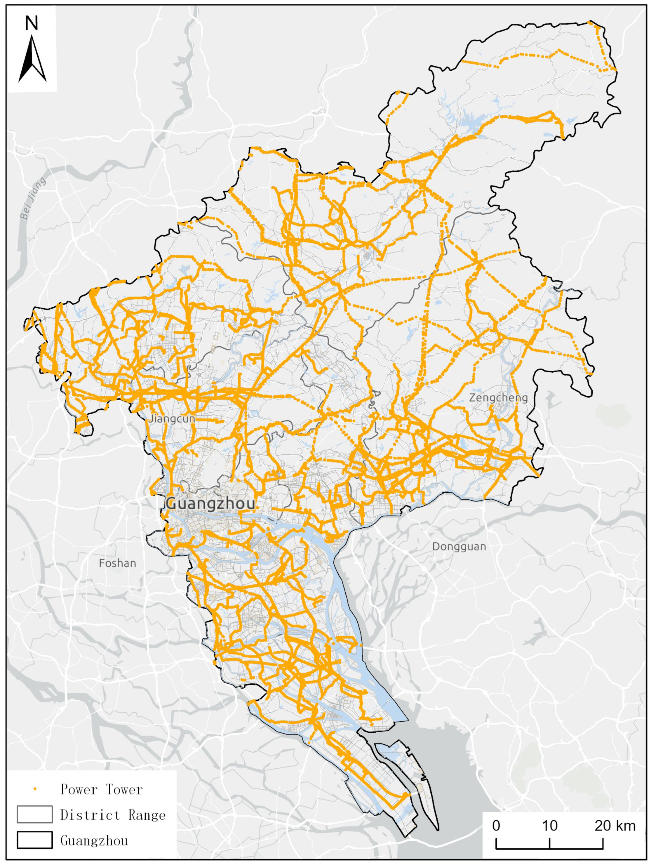
This study focuses on Guangzhou, China, as the research area (Figure 1). The spatial distribution data of power towers in Guangzhou were obtained from the open-source mapping platform OpenStreetMap (OSM). The dataset covers all 11 districts of Guangzhou and includes a total of 15,375 power towers. To accurately extract the distribution of transmission towers within each administrative district, boundary data for Guangzhou’s administrative divisions were retrieved from the National Geographic Information Resource Directory Service System of China.

Figure 1. Spatial distribution of power tower points in Guangzhou.

To assess various urban factors influencing tower distribution, multiple supplementary datasets were integrated: road network data were obtained from OSM; building footprint data were sourced from the dataset published by Zhang et al., with most source images acquired between 2022 and 2024 [42]; and population grid data were retrieved from the dataset by Chen et al., with a spatial resolution of 100 m × 100 m and no additional smoothing applied [43]. A detailed summary of all datasets used in this study, including version, license, and other provenance information, is provided in Table 1.

Table 1. Summary of datasets used in this study.

Dataset	Version/Date	Original CRS	License/Terms	URL	Access Date
Power tower locations (Guangzhou)	2025	WGS 1984 (EPSG: 4326)	OpenStreetMap License (ODbL)	https://www.openstreetmap.org	5 July 2025
Guangzhou administrative boundaries	2025	CGCS 2000 (EPSG: 4490)	National Geographic Information Resource Directory Service System of China	https://www.webmap.cn/main.do?method=index	3 July 2025
Road network data	2025	WGS 1984 (EPSG:4326)	OpenStreetMap License (ODbL)	https://www.openstreetmap.org	5 July 2025
Building footprint data	2022–2024	WGS 1984 (EPSG:4326)	Zhang et al. [42]	https://doi.org/10.6084/m9.figshare.27992417.v2	3 July 2025
Population grid data	2020	Albers Equal Area (Krassovsky 1942)	Chen et al. [43]	https://doi.org/10.6084/m9.figshare.24916140.v1	3 July 2025

For spatial consistency and comparability across all datasets, the geographic coordinate system used in this study is WGS 1984 (EPSG:4326), which provides a globally recognized reference for latitude and longitude measurements. All vector and raster data were reprojected to the Web Mercator projection (EPSG:3857) for spatial analyses, visualization, and mapping. This choice ensures that angular relationships are preserved, facilitates overlay operations across different datasets, and allows all experiments and analyses to be conducted within a unified coordinate system. By standardizing the spatial reference framework, potential errors arising from heterogeneous coordinate systems are eliminated, and distance, area, and spatial relationships remain comparable across datasets.

4. Methods

4.1. Workflow

This study utilizes multiple datasets, including population distribution, road networks, building footprints, and the spatial distribution of power towers in Guangzhou. A structured optimization framework for sensor deployment is proposed to support power grid condition monitoring. The framework employs buffer analysis and the entropy weight method to evaluate spatial correlations between transmission lines and urban features such as roads, buildings, and population density. A comprehensive risk score is calculated for each transmission tower using a weighted summation approach, and the resulting risk values are normalized to represent the monitoring demand intensity.

Based on the assessed monitoring demand, an integer programming model—the Backup Coverage Sensor Location Problem (BCSLP)—is formulated to ensure both complete coverage and system robustness in sensor deployment. To solve the model, this study applies two distinct solution methods: a genetic algorithm tailored to the characteristics of the power grid monitoring problem, and a commercial optimization solver (Gurobi). These approaches are independently implemented to obtain optimal or near-optimal deployment configurations under multiple constraints.

In this study, we restrict our analysis to homogeneous sensors, i.e., all sensors are assumed to have identical sensing range and deployment cost. This assumption allows us to focus on the core problem formulation and algorithm design without introducing additional heterogeneity-related complexity. The extension to heterogeneous sensor types with varying ranges and costs is an interesting and valuable direction, which we leave for future work.

This framework is risk-driven, spatially adaptive, and cost-aware, offering both theoretical and technical support for the scientific configuration of urban power grid sensor networks. The overall workflow is illustrated in Figure 2.

Figure 2. Workflow of the sensor deployment optimization for power grid condition monitoring.

4.2. BCSLP Model for Optimal Sensor Placement in Power Grid Monitoring

In power grid condition monitoring, the deployment of sensor networks is a key enabler for automated inspection and fault early warning. However, individual sensors may temporarily fail due to communication disruptions, hardware malfunctions, or extreme weather conditions. To ensure monitoring continuity for critical power grid assets, we introduce the Backup Coverage Sensor Location Problem (BCSLP) model. The core idea of this model is to guarantee that if a primary sensor fails, a backup sensor can seamlessly take over the monitoring task. This backup coverage ($\ge 2$ sensors) metric directly enhances system reliability by providing fault tolerance, ensuring a higher probability of detection even if a single sensor fails. This mechanism significantly improves the reliability and resilience of the monitoring network.

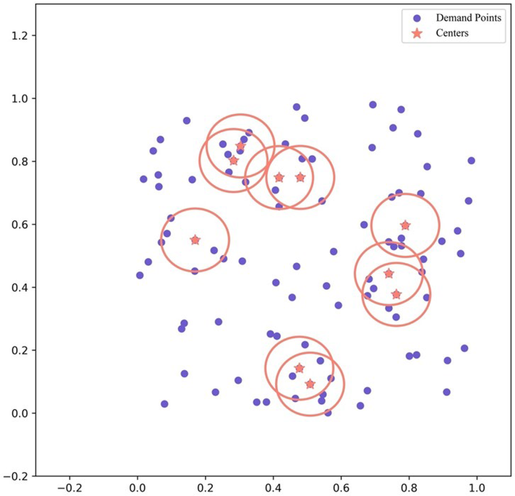
Figure 3 illustrates a conceptual example of the BCSLP model: the blue dots represent critical power grid assets (e.g., power towers), while the orange stars indicate selected sensor deployment sites. Each sensor has an effective monitoring radius (represented by orange circles), ensuring coverage of nearby assets.

Figure 3. An example of the BCSLP method (The red circles in the figure represent the coverage radius of the facilities).

The goal of optimal sensor deployment in power grid monitoring is to determine the best combination of sensor quantity and placement under a limited budget, in order to balance monitoring coverage and redundancy reliability. In this study, we formulate the problem as a Backup Coverage Sensor Location Problem (BCSLP), aiming to maximize the weighted coverage of critical grid assets. The requirement for backup coverage introduces redundancy, a fundamental principle for improving system reliability. This design ensures continuous monitoring capability and a significantly higher probability of detection in the event of an individual sensor failure. The model jointly considers the synergy between newly deployed and existing sensors.

Objective Functions:

$$Maximize Z_1={\displaystyle \sum _i}{a}_i{y}_i$$

(1)

$$Maximize Z_2={\displaystyle \sum _i}{a}_i{u}_i$$

(2)

Subject to:

$${\displaystyle \sum _{j\in N_i}}{x}_j\ge y_i, \forall i$$

(3)

$${\displaystyle \sum _{j\in N_i}}{x}_j-y_i\ge u_i, \forall i$$

(4)

$$u_i\le y_i, \forall i$$

(5)

$${\displaystyle \sum _j}{x}_j=P$$

(6)

$$x_j,y_i,u_i\in \left\{0,1\right\}, \forall i,j$$

(7)

• $i$: A critical power grid asset, such as a transmission tower, transformer, or switch station.
• $j$: A candidate site for sensor deployment.
• $x_j$: Binary decision variable; $x_j=1$ if a sensor is deployed at site $j$, otherwise $0$.
• $y_i$: Binary state variable; $y_i=1$ if asset $i$ is covered by at least one sensor (primary coverage).
• $u_i$: Binary state variable; $u_i=1$ if asset $i$ is redundantly covered by at least two sensors (backup coverage).
• $P$: Total budget limit for sensor deployment.
• $N_i$: Set of candidate locations capable of effectively monitoring asset $i$.
• $a_i$: Importance weight of asset $i$, which can be determined by factors such as voltage level, topological criticality, failure history, population served, or economic value.

Objective (1) aims to maximize the weighted primary coverage of all critical assets, ensuring wide monitoring coverage. Objective (2) seeks to maximize the weighted backup coverage, enhancing network robustness and resilience. Constraint (3) ensures that an asset is considered primarily covered only if it is within the range of at least one sensor. Constraint (4) defines backup coverage: an asset is backup-covered only if monitored by at least two sensors. Constraint (5) maintains logical consistency: backup coverage is allowed only if primary coverage is already achieved. Constraint (6) imposes a total budget cap. Constraint (7) ensures all decision variables are binary.

In practice, a weighted sum of the two objectives is often used to facilitate computation:

$$Maximize Z=\omega {\displaystyle \sum _i}{a}_i{y}_i + \left(1-\omega \right){\displaystyle \sum _i}{a}_i{u}_i$$

(8)

where $\omega \in \left[0,1\right]$ is a strategy weight parameter. When $\omega$ is close to 1, the model prioritizes coverage breadth, seeking to cover as many assets as possible. When $\omega$ is close to 0, the model emphasizes coverage reliability, ensuring redundancy for key assets. The value of $\omega$ can be adjusted based on the actual needs of decision-makers—e.g., broad-scale inspection versus targeted critical asset protection.

In our modeling, we note that the locations of existing towers do not automatically guarantee that their access, right-of-way, or safety meet the project requirements. These factors are treated as potential constraints. In practice, when metadata for a site (e.g., permit expiration, structural deficiency reports) is available and indicates infeasibility, we enforce the exclusion of such sites from the candidate set by setting their decision variable to zero (i.e., $x_j=0$).

4.3. Risk Heterogeneity and the Construction of a Multi-Dimensional Monitoring Priority Evaluation System

The operational risk of transmission towers in urban environments is inherently heterogeneous. Differences in geographic location, proximity to surrounding infrastructure, and local population density lead to substantial variation in both the potential consequences of incidents and the urgency of monitoring. To enable sensor deployment to respond precisely to spatial risk disparities and optimize resource allocation, this study constructs a comprehensive multi-dimensional monitoring priority evaluation system. The goal is to objectively quantify the monitoring value of each transmission tower, thereby guiding the optimization model to allocate limited sensing resources to the most critical nodes.

To achieve a standardized evaluation across diverse data sources and ensure fine-grained spatial assessment, the entire study area was discretized into a uniform grid of 100 m × 100 m resolution [44]. This spatial scale effectively captures local heterogeneity in risk and population distribution while maintaining computational efficiency. Each grid cell was treated as a basic analytical unit, within which two core indicators were calculated: (1) a composite risk score derived from proximity to roads and buildings, and (2) the population count within the cell. The former reflects the structural and operational risk associated with infrastructure interference, while the latter directly correlates with the potential impact of incidents on public safety and property.

To integrate multiple indicators, the Entropy Weight Method (EWM) was employed for weight determination [45]. EWM quantifies the informational contribution of each indicator by calculating its information entropy, assigning higher weights to indicators with greater variation and discriminatory power. The method involves a systematic procedure. First, all raw data $X=\left(x_{ij}\right)$, where i denotes the grid cell and $j$ the indicator, are normalized to the [0, 1] range to eliminate differences in magnitude and units. For positively oriented indicators, the normalization is performed using the following formula:

$$x_{ij}={\displaystyle \frac{x_{ij}-\min \left(x_j\right)}{\max \left(x_j\right)-\min \left(x_j\right)}}$$

(9)

This ensures comparability across all indicators. Next, the proportion $p_{ij}$ of each grid cell $i$ under indicator $j$ is computed to derive the information entropy $e_j$, as follows:

$$p_{ij}={\displaystyle \frac{x_{ij}}{{\sum }_i^m{x}_{ij}}}, e_j=-k {\displaystyle \sum _{i=1}^m}{p}_{ij}\ln \left(p_{ij}\right)$$

(10)

where $k={\displaystyle \frac{1}{ln\left(m\right)}}$, and $\mathrm{m}$ is the total number of grid cells. When $p_{ij}=0$, the term $p_{ij}ln\left(p_{ij}\right)$ is defined to be zero. A lower entropy value $e_j$ implies higher variation and greater informational value of the corresponding indicator.

Subsequently, the entropy weight $w_j$ for each indicator is calculated based on its redundancy $d_j=1-e_j$, as follows:

$$w_j = {\displaystyle \frac{1-e_{ij}}{{\sum }_{j=1}^n \left(1-e_j\right)}}$$

(11)

Using the derived objective weights $w_j$, a comprehensive monitoring priority score $S_i$ for each grid cell is calculated via a weighted sum:

$$S_i={\displaystyle \sum _j^n}{w}_j\cdot x_{ij}$$

(12)

The score $S_i$ reflects the overall monitoring urgency of the cell and is assigned to all power towers located within the corresponding grid. To eliminate scale effects and enhance interpretability, these scores are normalized so that $\sum a_i=1$. This normalization allows the weights to be interpreted as relative demand intensities and ensures comparability across demand points. The resulting normalized values are subsequently incorporated into the BCSLP optimization model as the importance coefficients $a_i$ for demand points.

Through this systematic data integration and analysis process, complex risk-related factors are transformed into a data-driven, quantifiable parameter that directly supports sensor deployment decisions. After normalization, the monitoring priority scores are converted into the demand weights $a_i$, which serve as importance coefficients in the optimization model. This ensures that the optimization solutions are guided by scientific, risk-oriented, and evidence-based criteria.

Taking Haizhu District of Guangzhou as an example, the spatial distribution of the normalized weight $a_i$ is shown below (Figure 4), and the overall frequency characteristics of $a_i$ are further summarized in the histogram (Figure 5). The histogram illustrates the overall numerical distribution of $a_i$ across all towers, while the heatmap intuitively reflects their spatial variation and clustering patterns. These results indicate that the $a_i$ values of power towers in Haizhu District exhibit notable variations both numerically and spatially.

Figure 4. Heatmap of the spatial distribution of demand weights $a_i$ in Haizhu District, Guangzhou.

Figure 5. Histogram of demand weights $a_i$ in Haizhu District, Guangzhou.

5. Experiment

5.1. Risk Assessment of Power Towers

5.1.1. Risk Zones near Roads for Power Towers in Guangzhou

Based on the integration of road networks and power tower data in Guangzhou, a 50 m buffer analysis was conducted to identify potential risk zones in proximity to roads (see Figure 6). In this study, a 50 m buffer around roads and buildings was adopted based on the following considerations: first, this distance effectively captures the immediate and most significant impact zone of traffic and construction activities; second, the 50 m threshold is widely applicable in spatial analysis and planning practices, ensuring both the rationality of impact identification and the operational feasibility of the results; finally, this distance is consistent with the control ranges commonly used in management regulations and planning practices. Therefore, a 50 m buffer was used as the standard in this study, and no additional sensitivity analysis with alternative distances (e.g., 25 m or 100 m) was conducted, in order to maintain consistency with practical management scales and ensure interpretability of the results. The spatial pattern exhibits characteristics of “core clustering, arterial extension, and dispersed periphery”: in core urban areas such as Yuexiu and Liwan districts, risk zones are densely distributed in patch-like forms, covering major commercial zones; along major arteries such as Huangpu Avenue and Guangzhou Avenue, risk zones extend linearly; in suburban areas like Zengcheng and Conghua, risk zones are scattered, reflecting a lack of safety planning for transmission towers in rural road expansion projects and revealing insufficient spatial regulation of peripheral power infrastructure.

Figure 6. Spatial Distribution Map of Road-Near Risk Zones for Power Towers in Guangzhou.

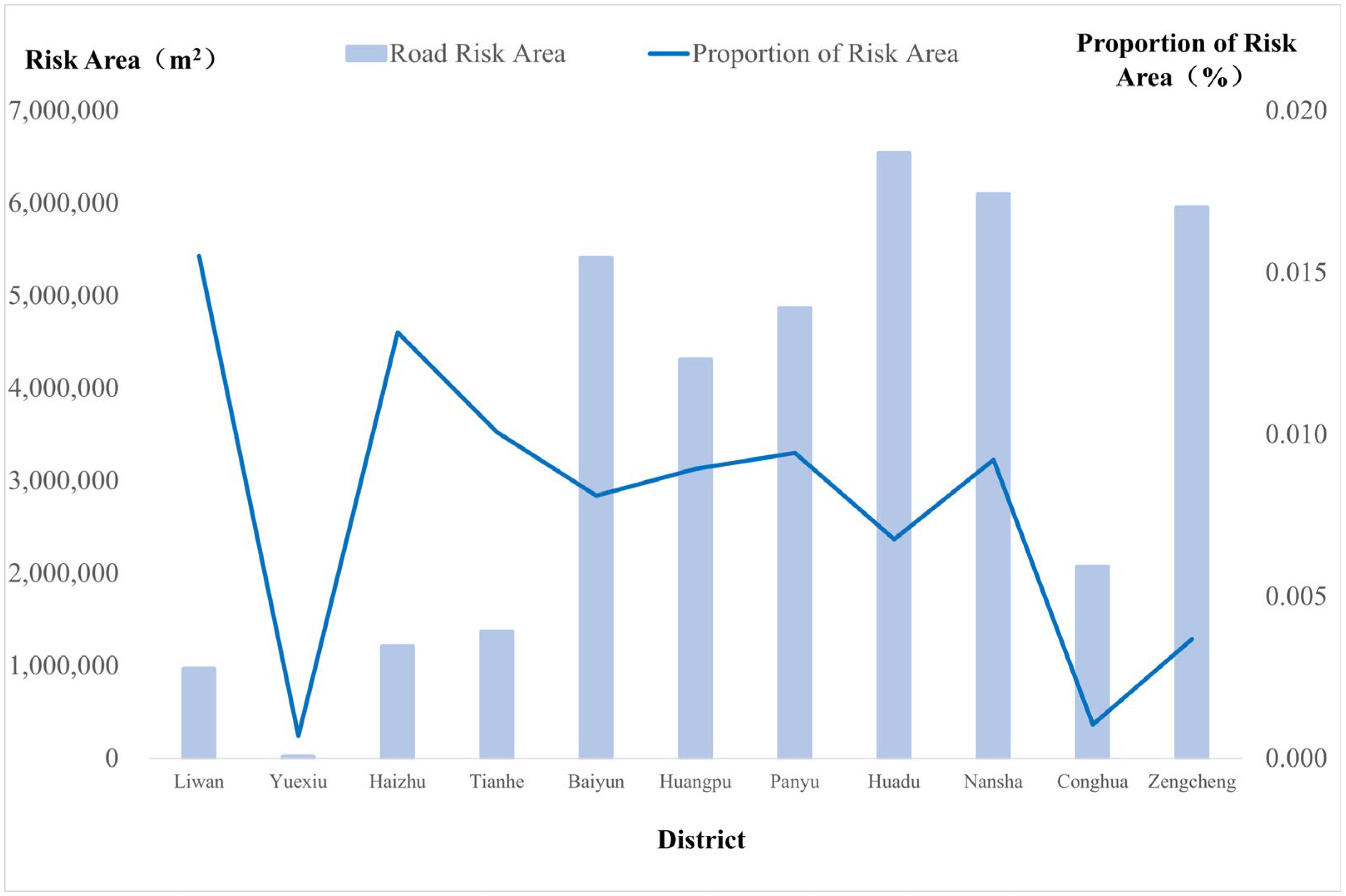
The total area of road-adjacent risk zones amounts to 38.825 million square meters. Huadu District (6.541 million m²) and Nansha District (6.098 million m²) have the largest absolute risk zone areas, while Liwan (1.55%) and Haizhu (1.31%) exhibit the highest risk density, indicating that dense road networks and insufficient safety distances from towers in older urban cores necessitate prioritized deployment of high-precision sensors (Figure 7). Although Zengcheng and Conghua have relatively large risk zone areas, their proportions are only 0.37% and 0.10%, respectively, suggesting a sparse and weak coverage of power infrastructure along rural roads. This calls for dynamic deployment strategies to address the limitations of traditional centralized monitoring, thereby reducing inspection blind spots and the risk of missed detections.

Figure 7. Statistical Chart of Road-Near Risk Zone Areas in Guangzhou.

5.1.2. Risk Zones near Buildings for Power Towers in Guangzhou

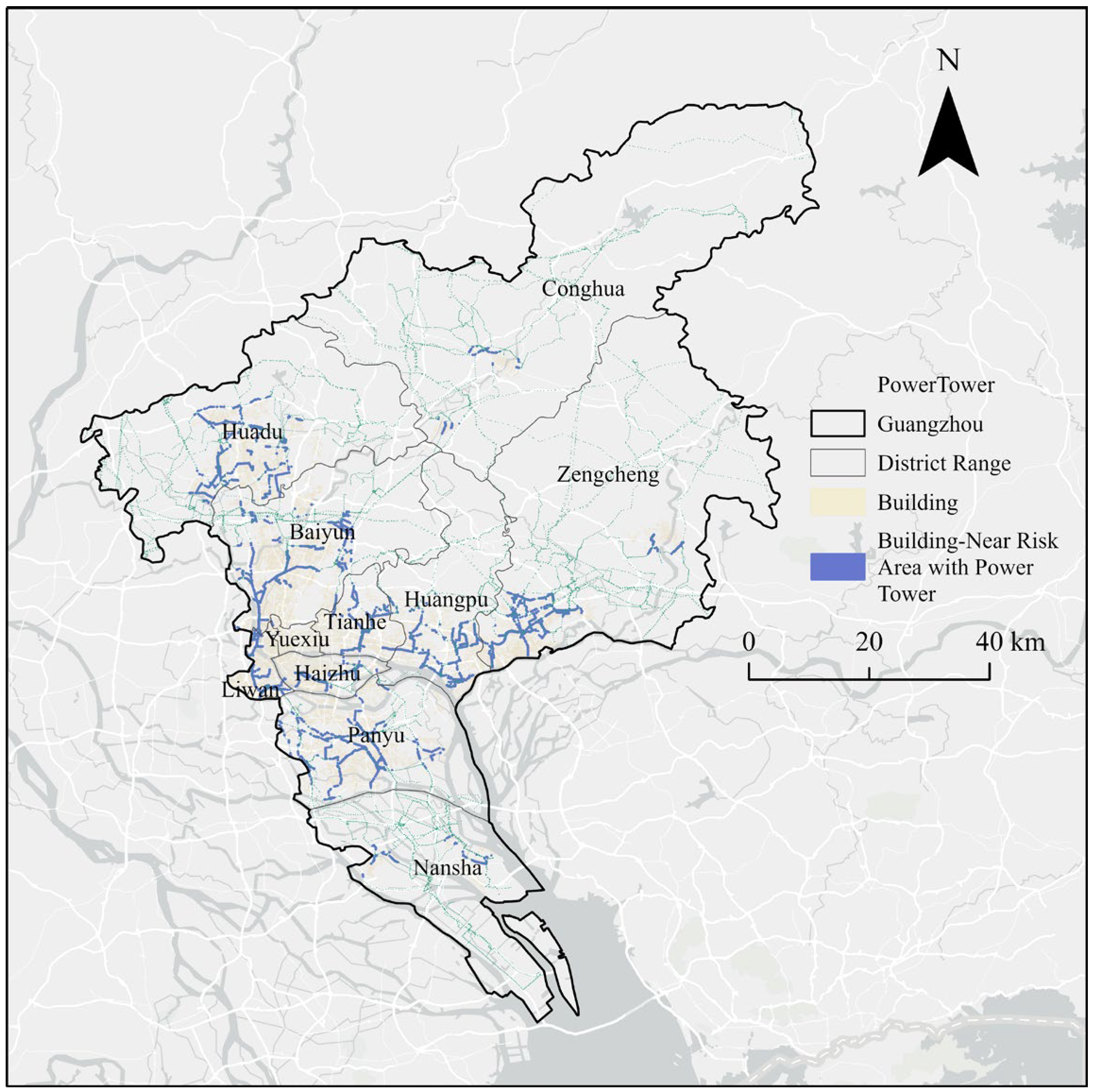
Based on a spatial overlay analysis of building footprints and power towers in Guangzhou, 50 m buffers were generated around each to identify potential risk zones where towers are in close proximity to buildings, as illustrated in Figure 8. From a spatial pattern perspective, these tower–building risk zones exhibit a multi-level structure characterized by “contiguous coverage in old urban areas—clustered distribution in urban villages—scattered patches in newly developed districts”. In historical districts such as Xiguan in Liwan and Xiaobei in Yuexiu, the risk zones are mainly concentrated in continuous polygonal areas. In contrast, in urban villages like Jiangxia (Baiyun District) and Tangxia (Tianhe District), dense “handshake” buildings form distinct clustered risk zones, significantly increasing the complexity of safety management for power infrastructure. In newly developed areas, risk zones are more sporadically distributed, reflecting the current lack of spatial coordination between new buildings and existing power facilities, which results in potential blind spots in safety coverage. This dispersed pattern highlights the need for greater flexibility in sensor deployment to avoid monitoring gaps caused by sparse layouts.

Figure 8. Spatial Distribution of Building-Near Risk Zones around Power Towers in Guangzhou.

The total area of building-near risk zones across the city reaches 16.035 million square meters, forming a stratified spatial distribution of “contiguous zones in old towns—clustered hotspots in urban villages—scattered patches in new districts”. Baiyun District (2.817 million m²) and Zengcheng District (2.665 million m²) contain the largest aggregated risk areas, whereas the highest risk density is found in Liwan District (2.04%), underscoring the inherent deficiencies in power facility safety planning in historical urban layouts (Figure 9). The high-risk clusters in urban villages are a result of their uniquely dense building patterns. Although the number of risk points is relatively low in newly developed areas such as Nansha (0.06%) and Conghua (0.01%), these zones may still pose significant safety hazards due to potential management oversights.

Figure 9. Statistical Chart of Building-Near Risk Zones in Guangzhou.

5.1.3. Comprehensive Risk Zones Around Power Towers in Guangzhou

Based on the spatial overlay analysis of power tower distribution, the combined effect of road-near and building-near risk zones reveals significant spatial heterogeneity in the potential risk pattern of Guangzhou’s power infrastructure. Overall, the distribution of towers exhibits a “sparse center–dense periphery” pattern (Figure 10). In central urban districts such as Yuexiu (3 towers) and Liwan (232 towers), high development density and a high degree of infrastructure undergrounding limit the available surface space for tower placement. These constraints impose higher requirements for the flexibility of grid inspection and the redundancy of monitoring safety. In contrast, peripheral districts like Huadu (2494 towers), Zengcheng (3057 towers), and Conghua (2392 towers) concentrate more than half (51.4%) of the city’s towers, primarily driven by rapid urban expansion and increasing power transmission demands. These areas form the physical basis for potential grid operation risks.

Figure 10. Spatial Distribution Map of Comprehensive Risk Zones near Power Towers in Guangzhou.

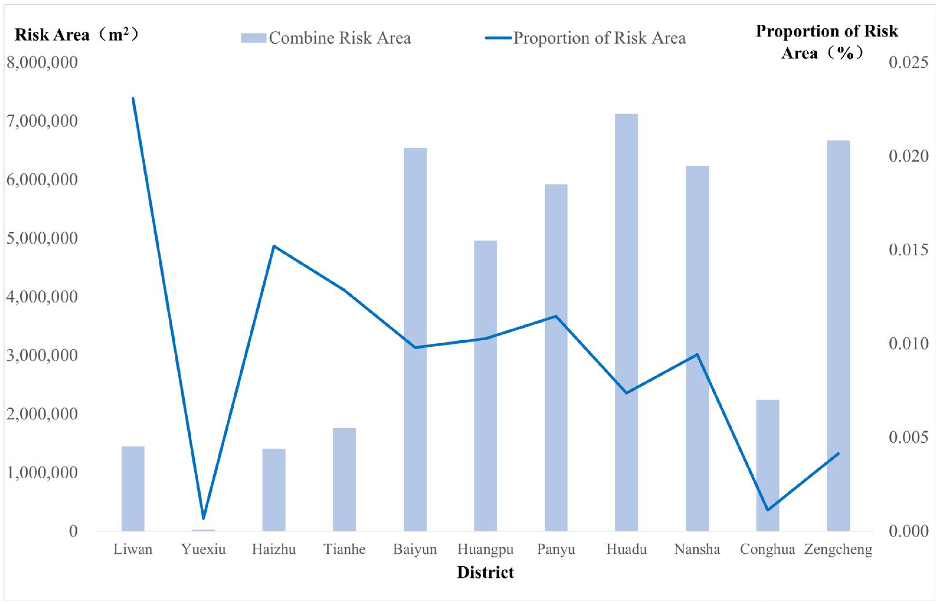
From the perspective of the overall spatial pattern, the distribution of risk zones closely overlaps with the areas of tower concentration. The three major peripheral districts—Huadu (7.119 million m²), Zengcheng (6.660 million m²), and Nansha (6.228 million m²)—together account for 61.2% of the total risk zone area in the city, reflecting both a high concentration of facilities and substantial spatial expansion pressure. This highlights a direct coupling relationship between power infrastructure deployment and spatial development dynamics (Figure 11). Meanwhile, central districts such as Yuexiu, despite their relatively small total risk area (23,000 m²), are characterized by dense development and spatial constraints, thereby requiring higher precision and flexibility in sensor deployment for effective monitoring coverage.

Figure 11. Statistical Chart of Comprehensive Risk Zone Areas around Power Towers in Guangzhou.

5.2. Solution of the BCSLP Model

The overall objective of this study is to develop an optimized sensor deployment strategy for monitoring the entire power transmission tower network in Guangzhou. However, the optimization of spatial sensor layouts inherently belongs to the class of NP-hard problems [46], whose computational complexity increases exponentially with the number of demand points and candidate facility sites. Given that there are 15,375 power towers distributed across Guangzhou, the sheer scale of the problem poses a significant computational challenge to obtaining exact optimal solutions within a reasonable timeframe. Even when heuristic algorithms are employed, achieving stable and efficient solutions remains difficult.

To ensure the feasibility of validating the model while enabling a more detailed and refined analysis of the optimization results, this study selects Haizhu District—a representative area of Guangzhou—as the experimental region. The choice of Haizhu District is based on the following considerations: Representativeness and Complexity: Haizhu is one of the core urban districts of Guangzhou, characterized by a complex urban fabric that includes densely populated old residential areas, emerging commercial centers, and major transportation hubs. The district exhibits a high density of transmission towers and diverse risk factors. Computational Feasibility: By narrowing the study area to Haizhu District (which contains 298 power towers), the problem scale becomes computationally manageable, allowing us to employ the Gurobi exact solver to obtain globally optimal solutions. These solutions can then serve as benchmarks for evaluating the performance of heuristic algorithms such as the genetic algorithm.

In this study, the candidate-site set $j$ was defined exclusively as the set of existing transmission tower locations within the study area. Since these towers already represent established infrastructure, additional site-screening criteria such as accessibility, rights-of-way, or safety were not applied.

All experiments in this section are conducted using the Haizhu District dataset. We employ two solution methods for the BCSLP model: Exact Algorithm: The industry-leading Gurobi optimizer is used to solve the mixed-integer linear programming (MILP) model, providing exact, provably optimal solutions [47]. Heuristic Algorithm: An improved Genetic Algorithm (GA) is applied as a comparative method. It is capable of producing high-quality near-optimal solutions within shorter computational times, demonstrating its potential for scaling up to larger regions in future applications [48]. All experiments were conducted on a Windows 11 workstation equipped with an Intel Core i7-14700F CPU (Intel, Santa Clara, CA, USA), an NVIDIA GeForce RTX 4060 Ti (8 GB) GPU (NVIDIA, Santa Clara, CA, USA), and 32 GB RAM. Optimization was performed with Gurobi Optimizer 12.0.3 via Python 3.10.16. The scientific stack comprised NumPy 1.26.4, Pandas 2.2.3, Matplotlib 3.10.0, Seaborn 0.13.2, and scikit-learn 1.7.0. Geospatial data processing used GeoPandas 1.0.1, Shapely 2.0.7, Fiona 1.10.1, and PyProj 3.7.1 on projected vector datasets (EPSG:3857). Desktop GIS tasks, including cartographic refinement and map export, were carried out in ArcGIS Pro 3.5.3.

5.2.1. Gurobi-Based Sensitivity Analysis of Weight ω and Knee-Point Identification for Primary–Backup Coverage Trade-Offs

This study conducts a sensitivity analysis by varying the weight parameter ω in the BCSLP to balance two core objectives: coverage breadth—maximizing the demand served at least once—and monitoring resilience—maximizing redundant monitoring of high-priority towers. We examine four representative strategies with $\mathsf{\omega }\in \{1.0,0.8,0.6,0.4,0.2,0.0\}$ and report results across budgets $\mathrm{P}\in \{20,25,30,35\}$. Primary covered demand (%) is defined as the share of aggregate demand served at least once within the service radius; backup covered demand (%) is the share served at least twice. All metrics are computed at the demand-point level with point-specific weights and then aggregated (Table 2).

Table 2. Computational results for the BCSLP performed by Gurobi.

$\mathit{w}$	$\mathit{P}$	Primary Covered Demand (%)	Backup Covered Demand (%)	Obj Value
1.0	20	84.2	3.00	11.8
1.0	25	92.4	2.50	13.0
1.0	30	97.1	4.80	13.7
1.0	35	99.3	7.70	14.0
0.8	20	80.3	2.20	9.65
0.8	25	89.3	27.6	10.8
0.8	30	93.2	39.5	11.6
0.8	35	95.2	52.9	12.2
0.6	20	70.8	40.0	8.22
0.6	25	81.7	44.1	9.38
0.6	30	86.7	54.0	10.4
0.6	35	92.3	60.5	11.2
0.4	20	58.2	52.9	7.74
0.4	25	68.7	58.8	8.83
0.4	30	73.7	67.4	9.83
0.4	35	79.4	74.5	10.8
0.2	20	56.9	53.5	7.62
0.2	25	64.4	61.1	8.69
0.2	30	71.7	68.3	9.70
0.2	35	77.4	75.3	10.7
0.0	20	56.4	53.5	7.52
0.0	25	64.2	61.1	8.60
0.0	30	68.9	68.4	9.63
0.0	35	76.6	75.4	10.6

When $\mathsf{\omega }=1.0$, the model is fully breadth-oriented. As the budget increases from $\mathrm{P}=20$ to 35, primary coverage climbs from 84.2% to 99.3%, while backup coverage remains low (3.0% to 7.7%); the objective value rises from 11.8 to 14.0. This pattern indicates dispersed deployments that prioritize serving as many distinct towers as possible at least once. The downside is limited redundancy: a single sensor failure can fully compromise monitoring in locally covered areas, which is undesirable for reliability-critical assets. At the opposite extreme ($\mathsf{\omega }=0.0$), the model fully prioritizes resilience. At $\mathrm{P}=20$, primary and backup coverage are 56.4% and 53.5%, and by $\mathrm{P}=35$ they reach 76.6% and 75.4%, respectively (objective 7.52 to 10.6). The resulting layouts concentrate sensors around high-risk towers to form multi-redundant clusters, ensuring robust coverage of core nodes but reducing breadth over peripheral or lower-risk towers.

Intermediate weights produce smooth and interpretable trade-offs. With ω = 0.8, from $\mathrm{P}=20$ to 35, primary increases from 80.3% to 95.2% while backup grows from 21.0% to 52.9% (objective 9.65 to 12.2); with $\mathsf{\omega }=0.6$, the same budgets yield 70.8% to 92.3% primary and 39.9% to 60.5% backup (8.22 to 11.2). As $\mathsf{\omega }$ decreases further, redundancy strengthens markedly: at $\mathrm{P}=35$, backup coverage reaches 74.5% for $\mathsf{\omega }=0.4$ and 75.3% for $\mathsf{\omega }=0.2$, while primary remains moderate (79.4% and 77.4%). Two additional observations follow. First, at any fixed budget, backup coverage rises rapidly as $\mathsf{\omega }$ decreases, with diminishing returns between $\mathsf{\omega }=0.2$ and $\mathsf{\omega }=0.0$, suggesting that extreme resilience pays little more than a resilience-biased balance. Second, within each ω, the objective value grows monotonically with $\mathrm{P}$, confirming scalability.

Taken together, the ⟨primary, backup⟩ frontiers reveal a knee-point around $\mathsf{\omega }=0.4$, identified using the Kneedle algorithm. This setting yields substantial breadth (≈$79\text{–}87\%$ across budgets) while also ensuring high redundancy (≈$53\text{–}75\%$). In other words, globally fixed $\mathsf{\omega }=0.4$ represents a reproducible compromise point between the extremes of breadth and resilience.

Accordingly, the subsequent improved genetic algorithm implementation focuses on the scenario where $\mathsf{\omega }=0.4$, not because it proved most effective in terms of raw objective values, but because it corresponds to the knee-point of the trade-off frontier. Unless otherwise specified, the subsequent experiments in this study adopt $\mathsf{\omega }=0.4$.

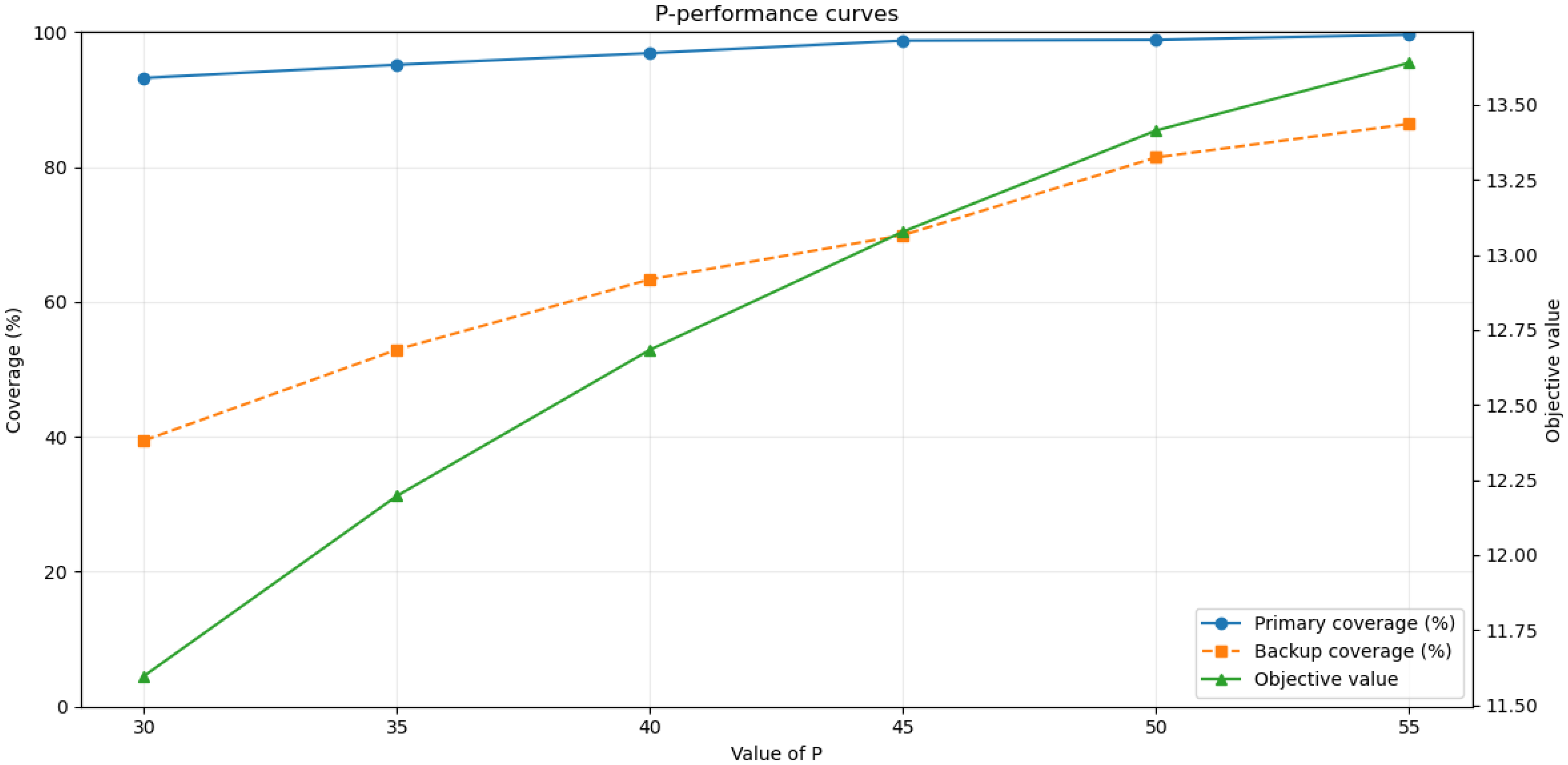
To examine the influence of different facility numbers, we tested $\mathrm{P}=[30,35,40,45,50,55]$ and constructed a performance curve shown below (Figure 12). The curve includes three key indicators: primary coverage, backup coverage, and the objective function value. The results show that all three indicators improve as the number of selected facilities increases, while the marginal gains gradually decrease, reflecting the trade-off between facility investment and coverage effectiveness.

Figure 12. Performance curves of primary $\mathrm{coverage}(\ge 1)$, backup $\mathrm{coverage}(\ge 2)$, and objective function with increasing facility numbers $\mathrm{P}$ and fixed $\mathsf{\omega }=0.4$.

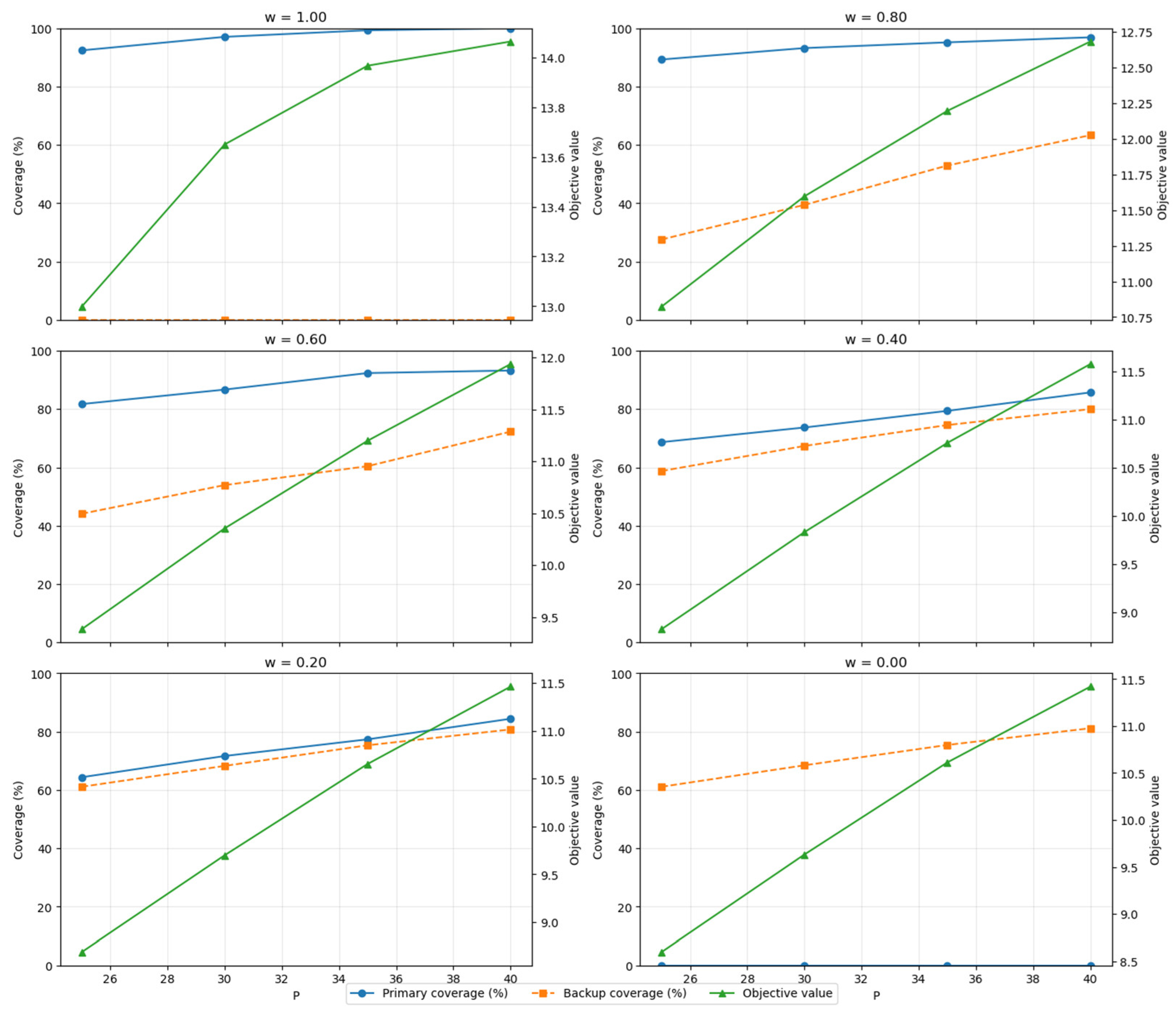
The figure below presents a comprehensive analysis of the impact of varying budget allocations on coverage metrics within the BCSLP framework (Figure 13).

Figure 13. Coverage performance (Primary coverage: $\ge 1$, Backup coverage: $\ge 2$) and objective values under varying $\mathrm{P}$ and weight $\mathsf{\omega }$.

Each subplot corresponds to a different $\mathsf{\omega }$, showing primary coverage (blue solid line), backup coverage (orange dashed line), and the overall objective value (green solid line) as functions of the budget. The results illustrate the trade-off between prioritizing primary versus backup coverage: when $\mathsf{\omega }$ is high, the model emphasizes maximizing primary coverage, while lower $\mathsf{\omega }$ values shift the solution toward improving redundancy. Within each $\mathsf{\omega }$, the objective value increases consistently with the budget, confirming scalability, while the trade-off plots highlight how different $\mathsf{\omega }$ shift the balance between breadth and redundancy. Selection of ω follows the knee-point rule introduced above, ensuring a reproducible balance.

In Figure 14 below, we compare solutions to the BCSLP obtained with the exact Gurobi solver under four facility budgets, $\mathrm{P}=25,30,35,40$. The background shows the demand surface (over-65 population) and the overlays mark the selected facilities and their service regions. Model settings are held fixed across panels: the coverage radius is 500 m, the objective weight is $\mathsf{\omega }=0.4$, and primary and backup coverage correspond to coverage by at least one and at least two facilities, respectively. As $\mathrm{P}$ increases, the selected sites densify along high-intensity demand corridors and clusters, expanding spatial reach while strengthening backup coverage near hotspots. The resulting deployment remains well dispersed, indicating that the model balances marginal coverage gains with redundancy under a consistent parameterization. Orange crosses denote selected facilities; orange circles delineate nominal 500 m service areas; the blue background encodes demand intensity. All panels are produced from the same candidate set and demand with identical parameters ($\mathsf{\omega }=0.4$; projected metric coordinates, EPSG:3857).

Figure 14. BCSLP site selection with the Gurobi solver under varying facility budgets ((a) P = 25, (b) P = 30, (c) P = 35, (d) P = 40) and fixed $\mathsf{\omega }=0.4$.

5.2.2. Heuristic Solution via an Improved Genetic Algorithm

While exact solvers such as Gurobi can deliver benchmark optimal solutions, their computational cost becomes prohibitive when dealing with large-scale, real-world instances of the BCSLP. To address this scalability challenge, we propose an enhanced Genetic Algorithm (GA), specifically tailored to the structural and computational complexities of the BCSLP model. Although traditional GAs are widely recognized for their global search capabilities, they often encounter difficulties in rugged fitness landscapes—such as premature convergence and the stochastic loss of elite individuals. To mitigate these limitations, our approach integrates a suite of synergistic strategies that collectively balance the trade-off between global exploration and local exploitation.

Rather than incorporating disparate algorithmic components, the proposed GA reflects a comprehensive redesign of the evolutionary process. First, an elitism mechanism is embedded to ensure stable and monotonic progress toward high-quality solutions. This strategy guarantees that the best-performing individuals are retained across generations, forming a robust solution baseline and safeguarding against performance deterioration due to random variation.

On this stable foundation, the algorithm employs an adaptive mutation strategy. By dynamically adjusting the mutation rate throughout the evolution process, the GA promotes thorough exploration in early stages—thus reducing the likelihood of premature convergence to sub-optimal solutions. As the population begins to converge on promising regions, the mutation rate is gradually decreased, facilitating a transition from global search to focused local refinement and enhancing convergence accuracy.

In parallel, a diversity control mechanism is incorporated to prevent genetic drift, which can occur when the population becomes dominated by a few highly similar individuals. By monitoring and regulating population diversity—specifically by identifying and limiting the proliferation of identical or near-identical chromosomes—this mechanism maintains a healthy level of genetic variance. As a result, the algorithm preserves its exploratory capacity and avoids entrapment in local optima, which is especially critical in complex, multi-modal spatial optimization landscapes.

These strategies transform the standard GA into a problem-aware and scalable optimization framework. The proposed algorithm demonstrates the ability to efficiently generate high-quality, near-optimal solutions for large-scale sensor placement scenarios—offering practical value for enhancing the resilience and safety of critical urban infrastructure systems.

We solve the Backup Coverage Location Problem using a tailored genetic algorithm. A chromosome encodes a feasible facility set of fixed cardinality p as a length-p list of distinct facility indices, and feasibility is preserved by all search operators. The population size is fixed at 50 individuals per generation and the run is terminated after 200 generations without additional early-stopping. Parent selection is rank-based: after sorting the population by fitness, 20 individuals form the mating pool via a probabilistic, rank-biased draw that favors higher-ranked solutions. Crossover is a set-preserving exchange applied at every mating event (effective crossover probability of 1.0): genes common to both parents are retained, while a randomly sized prefix (length cc chosen uniformly from the admissible range) of the non-overlapping subsequences is swapped between parents to produce one or two offspring; when parents are identical, only one child is created. Mutation is single-site and feasibility-preserving: with an adaptive probability ${\mathrm{p}}_{\mathrm{m}\mathrm{u}\mathrm{t}}\left(\mathrm{t}\right)=0.05+{\mathrm{p}}_0(1-\mathrm{t}/\mathrm{T})(\mathrm{w}\mathrm{i}\mathrm{t}\mathrm{h} {\mathrm{p}}_0=0.10,\mathrm{T}=200$, and $\mathrm{t}$ = the current generation), one randomly chosen gene is replaced by a facility index not present in the chromosome, which encourages exploration early (initial rate 0.15) and stabilizes to a 0.05 floor late in the run. Elitism retains the top two individuals from the mating pool via deep copy into the next generation, and the remaining slots are filled with offspring so that the population size remains constant. The algorithm returns the best-so-far solution and its objective value together with total runtime.

The following pseudocode summarizes the improved genetic algorithm used in this study (see Algorithm 1).

Algorithm 1: Improved GA for BSCLP (set-preserving crossover, elitism, adaptive mutation)
Inputs:
	$\mathrm{n} \left(\mathrm{d}\mathrm{e}\mathrm{m}\mathrm{a}\mathrm{n}\mathrm{d}\mathrm{s}\right), \mathrm{m} \left(\mathrm{c}\mathrm{a}\mathrm{n}\mathrm{d}\mathrm{i}\mathrm{d}\mathrm{a}\mathrm{t}\mathrm{e}\mathrm{s}\right), \mathrm{p} (\mathrm{s}\mathrm{i}\mathrm{t}\mathrm{e}\mathrm{s} \mathrm{t}\mathrm{o} \mathrm{s}\mathrm{e}\mathrm{l}\mathrm{e}\mathrm{c}\mathrm{t})$
	$\mathrm{D}\in \mathbb{R}^\{\mathrm{m}\times \mathrm{n}\} (\mathrm{f}\mathrm{a}\mathrm{c}\mathrm{i}\mathrm{l}\mathrm{i}\mathrm{t}\mathrm{y}-\mathrm{d}\mathrm{e}\mathrm{m}\mathrm{a}\mathrm{n}\mathrm{d} \mathrm{d}\mathrm{i}\mathrm{s}\mathrm{t}\mathrm{a}\mathrm{n}\mathrm{c}\mathrm{e}\mathrm{s}), \mathrm{r}>0 (\mathrm{c}\mathrm{o}\mathrm{v}\mathrm{e}\mathrm{r}\mathrm{a}\mathrm{g}\mathrm{e} \mathrm{r}\mathrm{a}\mathrm{d}\mathrm{i}\mathrm{u}\mathrm{s})$
	$\mathrm{d}\in \mathbb{R}^\mathrm{n}\text{\_}+ (\mathrm{d}\mathrm{e}\mathrm{m}\mathrm{a}\mathrm{n}\mathrm{d} \mathrm{w}\mathrm{e}\mathrm{i}\mathrm{g}\mathrm{h}\mathrm{t}\mathrm{s}), \mathrm{w}\in [0,1]$
	$\mathrm{G} (\mathrm{p}\mathrm{o}\mathrm{p}\mathrm{u}\mathrm{l}\mathrm{a}\mathrm{t}\mathrm{i}\mathrm{o}\mathrm{n} \mathrm{s}\mathrm{i}\mathrm{z}\mathrm{e}), \mathrm{R} (\mathrm{r}\mathrm{e}\mathrm{p}\mathrm{r}\mathrm{o}\mathrm{d}\mathrm{u}\mathrm{c}\mathrm{t}\mathrm{i}\mathrm{o}\mathrm{n} \mathrm{s}\mathrm{i}\mathrm{z}\mathrm{e} \le \mathrm{G}), \mathrm{T} \left(\mathrm{g}\mathrm{e}\mathrm{n}\mathrm{e}\mathrm{r}\mathrm{a}\mathrm{t}\mathrm{i}\mathrm{o}\mathrm{n}\mathrm{s}\right)$
	${\mathsf{\mu }}_0 (\mathrm{b}\mathrm{a}\mathrm{s}\mathrm{e} \mathrm{m}\mathrm{u}\mathrm{t}\mathrm{a}\mathrm{t}\mathrm{i}\mathrm{o}\mathrm{n} \mathrm{r}\mathrm{a}\mathrm{t}\mathrm{e}), \mathrm{E} \left(\mathrm{e}\mathrm{l}\mathrm{i}\mathrm{t}\mathrm{e}\mathrm{s}\right)$
Precompute:
	$\mathrm{A}\text{\_}\{\mathrm{j},\mathrm{i}\}=1\{\mathrm{D}\text{\_}\{\mathrm{j},\mathrm{i}\}\le \mathrm{r}\}\in \{0,1\}^\{\mathrm{m}\times \mathrm{n}\}$
	$\mathrm{d}\text{\_}\mathrm{t}\mathrm{o}\mathrm{t}=\sum \text{\_}\{\mathrm{i}=1\}^\mathrm{n} \mathrm{d}\text{\_}\mathrm{i} (>0)$
Coverage and objective:
	$\mathrm{F}\mathrm{o}\mathrm{r} \mathrm{S}\subset \left[\mathrm{m}\right], \left|\mathrm{S}\right|=\mathrm{p}:$
	$\mathrm{c}\text{\_}\mathrm{i}\left(\mathrm{S}\right)=\sum \text{\_}\{\mathrm{j}\in \mathrm{S}\}\mathrm{A}\text{\_}\{\mathrm{j},\mathrm{i}\}$
	$\mathrm{y}\text{\_}\mathrm{i}\left(\mathrm{S}\right)=1\{\mathrm{c}\text{\_}\mathrm{i}(\mathrm{S})\ge 1\}, \mathrm{u}\text{\_}\mathrm{i}\left(\mathrm{S}\right)=1\{\mathrm{c}\text{\_}\mathrm{i}(\mathrm{S})\ge 2\}$
	$\mathrm{P}\left(\mathrm{S}\right)=(\sum \text{\_}\{\mathrm{i}=1\}^\mathrm{n}\mathrm{d}\text{\_}\mathrm{i}·\mathrm{y}\text{\_}\mathrm{i}(\mathrm{S}\left)\right)/\mathrm{d}\text{\_}\mathrm{t}\mathrm{o}\mathrm{t} (\mathrm{p}\mathrm{r}\mathrm{i}\mathrm{m}\mathrm{a}\mathrm{r}\mathrm{y}\ge 1)$
	$\mathrm{B}\left(\mathrm{S}\right)=(\sum \text{\_}\{\mathrm{i}=1\}^\mathrm{n}\mathrm{d}\text{\_}\mathrm{i}·\mathrm{u}\text{\_}\mathrm{i}(\mathrm{S}\left)\right)/\mathrm{d}\text{\_}\mathrm{t}\mathrm{o}\mathrm{t} (\mathrm{b}\mathrm{a}\mathrm{c}\mathrm{k}\mathrm{u}\mathrm{p}\ge 2)$
	$\mathrm{f}\left(\mathrm{S}\right)=\mathrm{w}·\mathrm{P}\left(\mathrm{S}\right)+(1-\mathrm{w})·\mathrm{B}\left(\mathrm{S}\right) \left(\mathrm{m}\mathrm{a}\mathrm{x}\mathrm{i}\mathrm{m}\mathrm{i}\mathrm{z}\mathrm{e}\right)$
	$\mathrm{F}\mathrm{i}\mathrm{t}\mathrm{n}\mathrm{e}\mathrm{s}\mathrm{s}\left(\mathrm{S}\right)=-\mathrm{f}\left(\mathrm{S}\right)\left(\mathrm{m}\mathrm{i}\mathrm{n}\mathrm{i}\mathrm{m}\mathrm{i}\mathrm{z}\mathrm{e}\right)$
Operators:
	$\mathrm{S}\mathrm{e}\mathrm{l}\mathrm{e}\mathrm{c}\mathrm{t}\mathrm{i}\mathrm{o}\mathrm{n}(\mathrm{P}\mathrm{o}\mathrm{p},\mathrm{R}):\mathrm{a}\mathrm{n}\mathrm{y} \mathrm{s}\mathrm{t}\mathrm{a}\mathrm{n}\mathrm{d}\mathrm{a}\mathrm{r}\mathrm{d} \mathrm{s}\mathrm{c}\mathrm{h}\mathrm{e}\mathrm{m}\mathrm{e} (\mathrm{e}.\mathrm{g}., \mathrm{t}\mathrm{o}\mathrm{u}\mathrm{r}\mathrm{n}\mathrm{a}\mathrm{m}\mathrm{e}\mathrm{n}\mathrm{t})\to \mathrm{R} \mathrm{p}\mathrm{a}\mathrm{r}\mathrm{e}\mathrm{n}\mathrm{t}\mathrm{s}$
	$\mathrm{C}\mathrm{r}\mathrm{o}\mathrm{s}\mathrm{s}\mathrm{o}\mathrm{v}\mathrm{e}\mathrm{r}({\mathrm{S}}_1,{\mathrm{S}}_2,\mathrm{p}):\mathrm{s}\mathrm{e}\mathrm{t}-\mathrm{p}\mathrm{r}\mathrm{e}\mathrm{s}\mathrm{e}\mathrm{r}\mathrm{v}\mathrm{i}\mathrm{n}\mathrm{g}$
	$\mathrm{C}\text{\_}\mathrm{c}\mathrm{o}\mathrm{r}\mathrm{e}={\mathrm{S}}_1\cap {\mathrm{S}}_2; \mathrm{C}\text{\_}\mathrm{r}\mathrm{e}\mathrm{s}\mathrm{t}=({\mathrm{S}}_1\cup {\mathrm{S}}_2)\backslash \mathrm{C}\text{\_}\mathrm{c}\mathrm{o}\mathrm{r}\mathrm{e}$
	$\mathrm{K}=\mathrm{m}\mathrm{i}\mathrm{n}(\mathrm{p}-|\mathrm{C}\text{\_}\mathrm{c}\mathrm{o}\mathrm{r}\mathrm{e}|,|\mathrm{C}\text{\_}\mathrm{r}\mathrm{e}\mathrm{s}\mathrm{t}\left|\right)$
	$\mathrm{C}=\mathrm{C}\text{\_}\mathrm{c}\mathrm{o}\mathrm{r}\mathrm{e}\cup \mathrm{S}\mathrm{a}\mathrm{m}\mathrm{p}\mathrm{l}\mathrm{e}(\mathrm{C}\text{\_}\mathrm{r}\mathrm{e}\mathrm{s}\mathrm{t},\mathrm{K})$
	$\mathrm{i}\mathrm{f}\left|\mathrm{C}\right|<\mathrm{p}:\mathrm{f}\mathrm{i}\mathrm{l}\mathrm{l} \mathrm{f}\mathrm{r}\mathrm{o}\mathrm{m}\left[\mathrm{m}\right]\backslash \mathrm{C} \mathrm{u}\mathrm{n}\mathrm{i}\mathrm{f}\mathrm{o}\mathrm{r}\mathrm{m}\mathrm{l}\mathrm{y} \mathrm{t}\mathrm{o} \mathrm{s}\mathrm{i}\mathrm{z}\mathrm{e} \mathrm{p}$
	return C
	Mutation(S):
	$\mathrm{c}\mathrm{h}\mathrm{o}\mathrm{o}\mathrm{s}\mathrm{e} \mathrm{q}\in \{1,2\}; \mathrm{d}\mathrm{r}\mathrm{o}\mathrm{p} \mathrm{q} \mathrm{i}\mathrm{t}\mathrm{e}\mathrm{m}\mathrm{s} \mathrm{f}\mathrm{r}\mathrm{o}\mathrm{m} \mathrm{S}; \mathrm{a}\mathrm{d}\mathrm{d} \mathrm{q} \mathrm{f}\mathrm{r}\mathrm{o}\mathrm{m} \left[\mathrm{m}\right]\backslash \mathrm{S}; \mathrm{e}\mathrm{n}\mathrm{s}\mathrm{u}\mathrm{r}\mathrm{e}\left|\mathrm{S}\right|=\mathrm{p},\mathrm{u}\mathrm{n}\mathrm{i}\mathrm{q}\mathrm{u}\mathrm{e}$
	Adaptive rate:
	$\mathsf{\mu }\text{\_}\mathrm{t}=\mathrm{D}\mathrm{e}\mathrm{c}\mathrm{a}\mathrm{y}({\mathsf{\mu }}_0,\mathrm{t},\mathrm{T})(\mathrm{e}.\mathrm{g}.,\mathsf{\mu }\text{\_}\mathrm{t}=\mathrm{m}\mathrm{a}\mathrm{x}(\mathsf{\mu }\text{\_}\mathrm{m}\mathrm{i}\mathrm{n},{\mathsf{\mu }}_0·(1-\mathrm{t}/\mathrm{T})^\mathsf{\beta }\left)\right)$
Main loop:
	$\mathrm{I}\mathrm{n}\mathrm{i}\mathrm{t}\mathrm{i}\mathrm{a}\mathrm{l}\mathrm{i}\mathrm{z}\mathrm{e} \mathrm{P} \mathrm{w}\mathrm{i}\mathrm{t}\mathrm{h} \mathrm{G} \mathrm{r}\mathrm{a}\mathrm{n}\mathrm{d}\mathrm{o}\mathrm{m} \mathrm{s}\mathrm{i}\mathrm{z}\mathrm{e}-\mathrm{p} \mathrm{u}\mathrm{n}\mathrm{i}\mathrm{q}\mathrm{u}\mathrm{e} \mathrm{s}\mathrm{u}\mathrm{b}\mathrm{s}\mathrm{e}\mathrm{t}\mathrm{s} \mathrm{o}\mathrm{f} \left[\mathrm{m}\right]$
	$\mathrm{E}\mathrm{v}\mathrm{a}\mathrm{l}\mathrm{u}\mathrm{a}\mathrm{t}\mathrm{e} \mathrm{F}\mathrm{i}\mathrm{t}\mathrm{n}\mathrm{e}\mathrm{s}\mathrm{s}; \mathrm{s}\mathrm{e}\mathrm{t} \mathrm{S} *=\mathrm{a}\mathrm{r}\mathrm{g}\mathrm{m}\mathrm{i}\mathrm{n} \mathrm{F}\mathrm{i}\mathrm{t}\mathrm{n}\mathrm{e}\mathrm{s}\mathrm{s}\left(\mathrm{P}\right); \mathrm{H}\mathrm{i}\mathrm{s}\mathrm{t}\mathrm{o}\mathrm{r}\mathrm{y}=\left[\mathrm{f}\right(\mathrm{S}*\left)\right]$
	$\mathrm{f}\mathrm{o}\mathrm{r} \mathrm{t}=1..\mathrm{T}:$
	$\mathsf{\mu }\leftarrow \mathsf{\mu }\text{\_}\mathrm{t}; \mathrm{E}\mathrm{l}\mathrm{i}\mathrm{t}\mathrm{e}\leftarrow \mathrm{t}\mathrm{o}\mathrm{p} \mathrm{E} \mathrm{b}\mathrm{y} \mathrm{F}\mathrm{i}\mathrm{t}\mathrm{n}\mathrm{e}\mathrm{s}\mathrm{s}$
	$\mathrm{M}\leftarrow \mathrm{S}\mathrm{e}\mathrm{l}\mathrm{e}\mathrm{c}\mathrm{t}\mathrm{i}\mathrm{o}\mathrm{n}(\mathrm{P},\mathrm{R}); \mathrm{O}\leftarrow \mathrm{\varnothing }$
	$\mathrm{w}\mathrm{h}\mathrm{i}\mathrm{l}\mathrm{e} \left|\mathrm{E}\mathrm{l}\mathrm{i}\mathrm{t}\mathrm{e}\right|+\left|\mathrm{O}\right|<\mathrm{G}:$
	pick $({\mathrm{S}}_1,{\mathrm{S}}_2)$ from M
	C ← $\mathrm{Crossover}({\mathrm{S}}_1,{\mathrm{S}}_2,\mathrm{p})$
	with prob $\mathsf{\mu }:\mathrm{C}$ ← Mutation(C)
	$\mathrm{O}\leftarrow \mathrm{O}\cup \{\mathrm{C}\}$
	$\mathrm{P}\leftarrow \mathrm{E}\mathrm{l}\mathrm{i}\mathrm{t}\mathrm{e}\cup \mathrm{O}$
	$\mathrm{i}\mathrm{f} \mathrm{m}\mathrm{i}\mathrm{n} \mathrm{F}\mathrm{i}\mathrm{t}\mathrm{n}\mathrm{e}\mathrm{s}\mathrm{s}\left(\mathrm{P}\right) \mathrm{i}\mathrm{m}\mathrm{p}\mathrm{r}\mathrm{o}\mathrm{v}\mathrm{e}\mathrm{s}:\mathrm{u}\mathrm{p}\mathrm{d}\mathrm{a}\mathrm{t}\mathrm{e} \mathrm{S} *$
	$\mathrm{a}\mathrm{p}\mathrm{p}\mathrm{e}\mathrm{n}\mathrm{d} \mathrm{f}(\mathrm{S}*) \mathrm{t}\mathrm{o} \mathrm{H}\mathrm{i}\mathrm{s}\mathrm{t}\mathrm{o}\mathrm{r}\mathrm{y}$
Output:
	$\mathrm{S}* (\mathrm{s}\mathrm{e}\mathrm{l}\mathrm{e}\mathrm{c}\mathrm{t}\mathrm{e}\mathrm{d} \mathrm{i}\mathrm{n}\mathrm{d}\mathrm{i}\mathrm{c}\mathrm{e}\mathrm{s}),\mathrm{f}(\mathrm{S}*),\mathrm{H}\mathrm{i}\mathrm{s}\mathrm{t}\mathrm{o}\mathrm{r}\mathrm{y}(\mathrm{b}\mathrm{e}\mathrm{s}\mathrm{t}-\mathrm{s}\mathrm{o}-\mathrm{f}\mathrm{a}\mathrm{r}),\mathrm{r}\mathrm{u}\mathrm{n}\mathrm{t}\mathrm{i}\mathrm{m}\mathrm{e}$

Performance and Analysis of Improved GA

Figure 15 compares the convergence behavior of the genetic algorithm under four hyperparameter configurations, with the problem instance, objective definition, and weights held fixed. Each curve reports the mean best-so-far objective value over 200 generations, averaged across 20 independent runs for each configuration. The legend encodes generation size (gen), reproduction pool size (repr), base mutation probability before adaptive decay (mut), and the number of elites carried over each generation (elite). All configurations use the same set-preserving crossover at every mating event; runs differ only in their random seeds.

Figure 15. GA convergence under different hyperparameters.

Across all settings, the algorithm exhibits rapid improvement during the first 10–20 generations followed by diminishing returns, indicating that most gains are realized early while later generations mainly refine solutions. An increasing population and reproduction pool $(\mathrm{g}\mathrm{e}\mathrm{n}=80,\mathrm{r}\mathrm{e}\mathrm{p}\mathrm{r}=30,\mathrm{m}\mathrm{u}\mathrm{t}=0.10,\mathrm{e}\mathrm{l}\mathrm{i}\mathrm{t}\mathrm{e}=2)$ accelerates early progress and yields the highest terminal objective $(\approx 13.47)$, outperforming the baseline $(\mathrm{g}\mathrm{e}\mathrm{n}=50,\mathrm{r}\mathrm{e}\mathrm{p}\mathrm{r}=20,\mathrm{m}\mathrm{u}\mathrm{t}=0.10,\mathrm{e}\mathrm{l}\mathrm{i}\mathrm{t}\mathrm{e}=2;\approx 13.41)$. Raising the mutation rate to 0.20 (with other settings fixed) slightly speeds up early exploration but makes it converge to a marginally lower plateau $(\approx 13.38)$, consistent with stronger stochasticity trading off final refinement. Removing elitism $(\mathrm{e}\mathrm{l}\mathrm{i}\mathrm{t}\mathrm{e}=0)$ produces the slowest and lowest convergence ($\approx 13.35$), underscoring the stabilizing role of retaining top solutions. Overall, larger gen/repr and modest elitism provide the most reliable improvements, whereas overly aggressive mutation offers limited benefit at convergence. These trends suggest using moderate mutation with elitism and, when computationally affordable, a larger population to secure faster and higher-quality solutions.

Figure 16 illustrates the runtime of the improved GA under different population sizes P on the same hardware. The plot reports the median runtime together with the interquartile range $[{\mathrm{p}}_{25},{\mathrm{p}}_{75}]$. As shown, the runtime exhibits approximately linear growth as $\mathrm{P}$ increases. Specifically, when $\mathrm{P}=20$, the runtime is around 0.38 s, while for $\mathrm{P}=60$, it rises to about 0.94 s. These results indicate that enlarging the population size introduces additional computational overhead, but the overall runtime remains within an acceptable range for practical applications.

Figure 16. Runtime of the improved GA with varying population sizes $\mathrm{P}$, showing the median and the $\left[{\mathrm{p}}_{25},{\mathrm{p}}_{75}\right]$ interval.

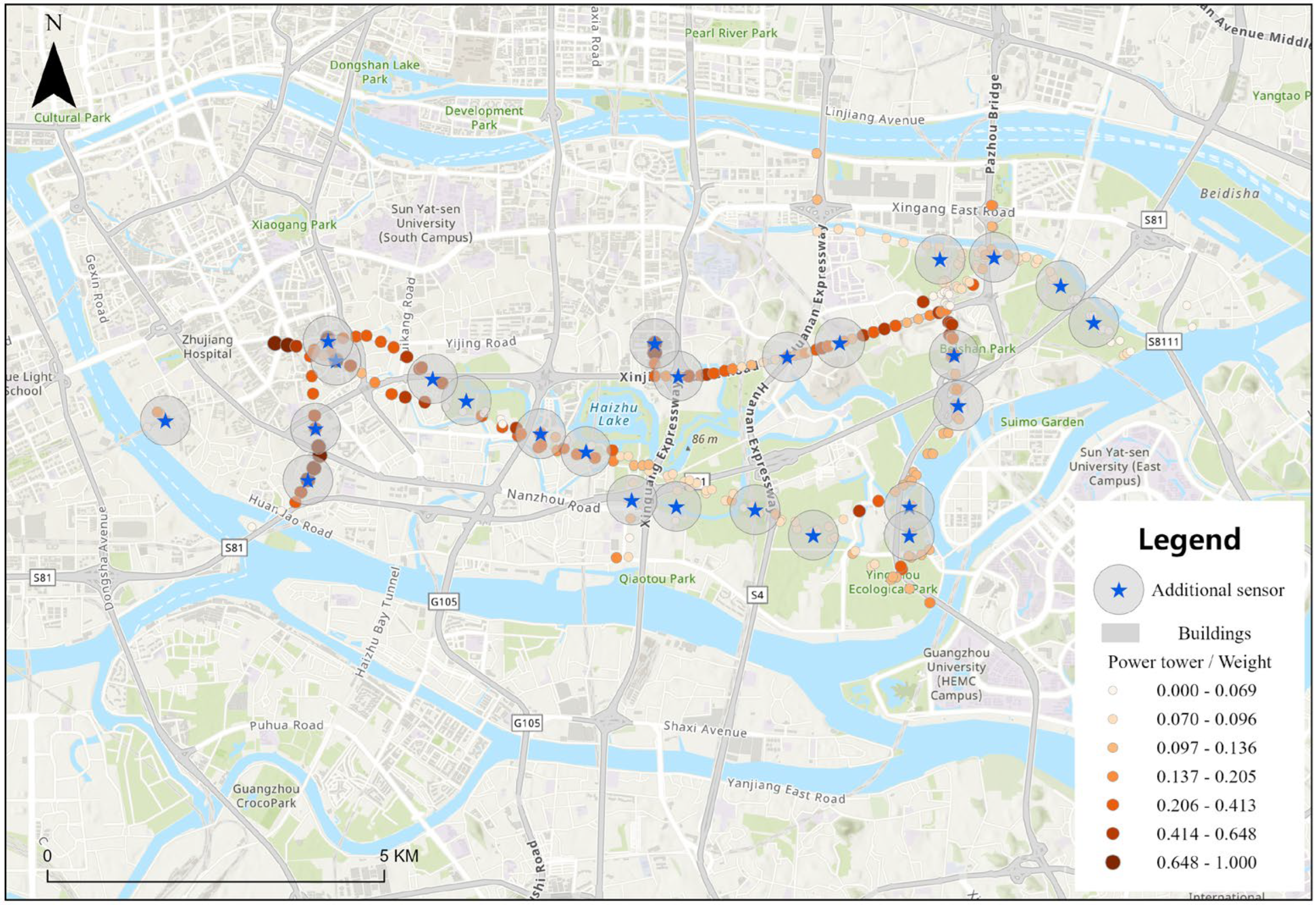
The optimized sensor placement solutions for the BCSLP obtained by the improved genetic algorithm are presented in Figure 17. The results demonstrate that the algorithm successfully identifies a subset of transmission towers that maximizes both primary and backup coverage, effectively reflecting the towers’ spatial risk distribution. High-risk towers, as quantified in the earlier risk analysis, are preferentially included in the selected facility set, indicating that the GA effectively balances coverage efficiency and redundancy. Overall, the solution confirms the capability of the improved GA to generate high-quality, near-optimal configurations, providing a practical basis for the implementation of resilient and risk-aware monitoring in urban power grids.

Figure 17. Results of the Solution Performed by Improved Genetic Algorithm.

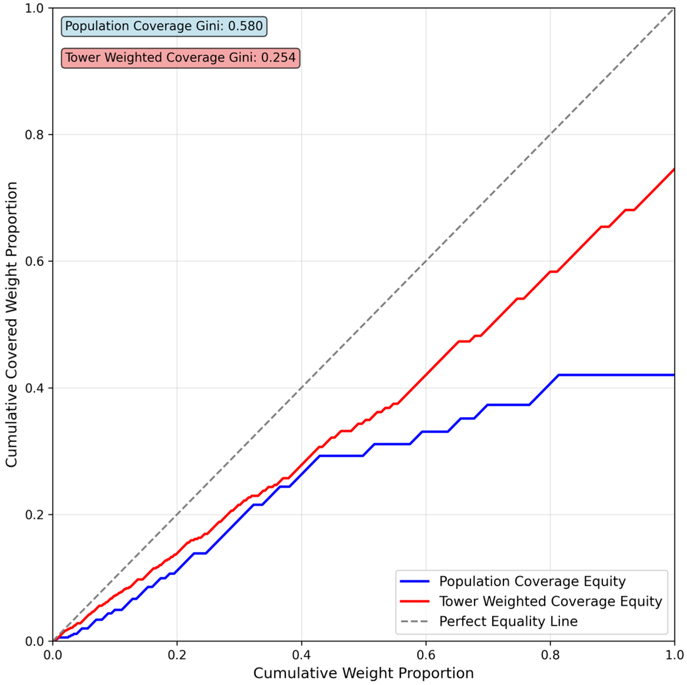
In facility location studies, equity represents a crucial dimension for evaluating the rationality of spatial configurations. Traditional optimization models typically emphasize maximizing coverage as the primary objective; however, an exclusive focus on efficiency may result in spatially uneven resource distribution, thereby leaving certain regions or population groups underserved. To quantitatively capture such inequalities, this study adopts the Gini coefficient as an equity assessment indicator [49]. Originally developed to measure income inequality, the Gini coefficient ranges from 0 to 1, with lower values indicating more equitable distributions and higher values reflecting greater disparities. In this study, the Gini coefficient is applied to evaluate the equity of tower location schemes in terms of both population coverage and tower-weight coverage. Specifically, population data for Zhuhai District are statistically analyzed and stratified to characterize spatial variations in population density, which are then compared with the tower coverage outcomes. For consistency, the service radius of tower monitoring facilities is uniformly set to 500 m, in alignment with the parameter settings described earlier.

The results (Figure 18) indicate that the Gini coefficient for population coverage is 0.58, suggesting that the current location scheme exhibits a certain degree of inequity across different population strata. This disparity was further confirmed by statistical testing $({\mathsf{\chi }}^2 \mathrm{t}\mathrm{e}\mathrm{s}\mathrm{t},p<0.01)$. By contrast, the Gini coefficient for tower-weight coverage is only 0.25, reflecting a substantially higher level of equity in terms of monitoring tower distribution. This implies that a limited number of selected sites can effectively cover the majority of high-weight towers, thereby ensuring both the fairness and effectiveness of tower monitoring. It is also worth noting that, in this study, power tower locations are generally situated in areas with relatively low population density, and the monitoring points are deployed directly on the towers. This contextual factor further supports the rationale of the equity analysis, as the monitoring coverage of towers can be considered balanced.

Figure 18. Lorenz curves of coverage distribution for population and towers.

Ablation Study: Evaluating Adaptive Mutation and Elitism in the Genetic Algorithm

To assess the effectiveness of our improvements to the genetic algorithm (GA) for the BCSLP, we conduct an ablation study that contrasts an Improved GA—equipped with adaptive mutation and elitism—against a Baseline GA without these components. Both algorithms operate on the same dataset, distance metric, and normalized coverage radius as the main experiments. Hyperparameters are aligned to ensure fair comparison (200 generations, population size 50, reproduction size 20, base mutation rate 0.10); the Improved GA uses an elitism size of 2 and an adaptive mutation schedule with a lower bound. To control randomness, we pair runs via matched seeds and repeat the experiment multiple times to limit stochastic variance. Evaluation focuses on the BCSLP objective (the weighted sum of primary and backup coverage), primary coverage (users covered by at least one facility), backup coverage (users covered by at least two facilities), and wall-clock runtime. The accompanying figure visualizes run-wise objective values across repetitions, enabling a direct comparison of central tendency and variability between the two methods.

Results (Figure 19) indicate that the Improved GA attains slightly higher objective values on average while exhibiting reduced run-to-run variance, reflecting more stable convergence behavior. Under the same computational budget, it typically reaches competitive solutions earlier, and its runtime remains comparable to that of the Baseline GA. These findings support the conclusion that adaptive mutation and elitism offer a robust, reproducible performance gain without incurring notable computational overhead.

Figure 19. Ablation Study: Objective across Runs (BaselineGA vs. ImprovedGA).

6. Discussion and Conclusions

6.1. Discussion

This study successfully developed and validated a risk-informed optimization framework for deploying condition monitoring sensors on urban power grids, using Guangzhou as a case study. The results not only provide specific layout strategies but also yield several significant insights into the strategic challenges of safeguarding critical infrastructure.

A principal finding is the critical trade-off between monitoring breadth and monitoring resilience. The sensitivity analysis, orchestrated by adjusting the weight parameter ω, quantitatively demonstrated the limitations of extreme strategies. A breadth-focused approach $(\mathsf{\omega }=1.0)$, while covering the maximum number of towers, creates a fragile network vulnerable to single-point failures—a risk that is unacceptable for critical infrastructure. Conversely, a purely resilience-focused strategy $(\mathsf{\omega }=0.0)$ leads to the inefficient clustering of resources around a few key nodes, leaving large portions of the grid unmonitored. Our findings strongly advocate for a balanced, resilience-biased strategy, which ensures that while a majority of assets receive baseline coverage, the most critical, high-risk towers are fortified with redundant monitoring. This nuanced approach aligns with modern resilience engineering principles, which prioritize system integrity under duress over simple coverage metrics.

The methodological strength of this study lies in its data-driven, objective approach to defining “criticality”. By employing the Entropy Weight Method (EWM) to synthesize composite risk from road/building proximity and population density, we moved beyond subjective or uniform assumptions. This ensures that the optimization is guided by quantifiable, spatially heterogeneous risk, making the resulting deployment plans directly relevant and defensible for urban planners and utility operators. The clear identification of high-risk zones in Haizhu District underscores the practical value of this granular, risk-aware prioritization.

Furthermore, the dual-solver approach validates both the model’s conceptual soundness and its practical scalability. The use of the Gurobi optimizer on the Haizhu District case study provided a provably optimal solution, serving as a crucial benchmark. The successful performance of our improved Genetic Algorithm (GA)—achieving near-optimal results with significantly lower computational overhead—is arguably the most critical outcome for future application. It demonstrates that the framework is not merely a theoretical construct but a viable tool that can be scaled to address the full complexity of metropolitan-scale networks like the entirety of Guangzhou.

Despite these contributions, we acknowledge several limitations that open avenues for future research. First, our analysis was confined to a single district; scaling the GA to the entire city is the logical next step. Second, the model utilized a uniform monitoring radius and cost structure, whereas in reality, terrain, signal obstruction, and installation complexity could introduce heterogeneous costs and coverage patterns. Future work could incorporate more sophisticated, variable-cost and variable-coverage functions. Finally, the risk assessment was static; a more advanced implementation could integrate dynamic data, such as real-time weather threats or historical failure rates, to enable dynamic and adaptive sensor deployment strategies.

Physical detection model and simplification. In practice, a sensor’s detectable footprint is determined by its emitted/received radiation pattern and an Signal-to-Noise Ratio (SNR) threshold, as well as line-of-sight availability, occlusion by buildings/terrain/vegetation, installation height and tilt, and environmental conditions (e.g., clutter, weather, background noise). A physically faithful treatment would propagate signal strength from each facility to each demand point in 3D, enforce visibility constraints, and declare coverage when the predicted SNR exceeds a threshold. In this study we adopt the standard disk-coverage abstraction widely used in facility location: a demand point $\mathrm{j}$ is considered covered by facility $\mathrm{i}$ if the planimetric distance is within a calibrated radius $\mathrm{r}$. This choice is motivated by: (i) data availability and identifiability—city-scale, temporally consistent 3D layers and noise/clutter fields are not uniformly available, whereas r can be calibrated from vendor specifications or pilot measurements; (ii) comparability with the literature—disk coverage is the de facto benchmark for backup-coverage models; and (iii) computational tractability—binary coverage within radius r yields a sparse set-cover structure, enabling efficient optimization at our spatial scale, whereas ray-tracing/SNR models would require repeated propagation solves and substantially increase runtime. We acknowledge that the disk model assumes isotropy, ignores line-of-sight and occlusion, and does not parameterize vertical patterns or mounting height; consequently, it may overestimate coverage in dense urban cores and underestimate it in open areas. Future work will incorporate 3D GIS (Digital Surface Model (DSM)/Digital Terrain Model (DTM)/buildings) for visibility-aware coverage, anisotropic sectors or elliptical footprints, and height-dependent propagation, e.g., by precomputing occlusion-aware visibility matrices or using differentiable propagation surrogates within the optimization.

6.2. Conclusions

This paper addressed the critical challenge of optimizing sensor placement for power grid condition monitoring by introducing a novel framework grounded in the principles of network resilience. We formulated a Backup Coverage Sensor Location Problem (BCSLP) model, which, unlike traditional coverage models, explicitly balances the dual objectives of maximizing both primary and backup monitoring of power towers. Pursuing backup coverage not only increases redundancy but also fundamentally boosts the network’s resilience against single-point failures, thereby providing more reliable early-warning capability.

By first constructing a data-driven, multi-dimensional risk profile for each power tower using the Entropy Weight Method (EWM), we ensured that the optimization was guided by objective measures of criticality. Through a detailed case study in Guangzhou’s Haizhu District, we demonstrated that a balanced strategy, prioritizing both coverage breadth and resilience, yields significantly more robust and practical deployment solutions than strategies focused on a single objective. Furthermore, we developed and validated an improved Genetic Algorithm that produces high-quality, near-optimal solutions efficiently, confirming the framework’s scalability for large-scale, real-world applications.

Ultimately, this research contributes a robust, scientifically grounded, and scalable decision-support tool for utility operators and urban planners. By enabling the strategic deployment of monitoring sensors, the proposed framework enhances the proactive maintenance capabilities and overall resilience of urban power grids, which are indispensable lifelines in modern smart cities.

References

1. Bibri, S.E.; Krogstie, J. Smart Sustainable Cities of the Future: An Extensive Interdisciplinary Literature Review. Sustain. Cities Soc. 2017, 31, 183–212. [Google Scholar] [CrossRef]
2. Yigitcanlar, T.; Kamruzzaman, M.; Buys, L.; Ioppolo, G.; Sabatini-Marques, J.; Da Costa, E.M.; Yun, J.J. Understanding ‘Smart Cities’: Intertwining Development Drivers with Desired Outcomes in a Multidimensional Framework. Cities 2018, 81, 145–160. [Google Scholar] [CrossRef]
3. Zhou, L.; Hu, F.; Wang, B.; Wei, C.; Sun, D.; Wang, S. Relationship between Urban Landscape Structure and Land Surface Temperature: Spatial Hierarchy and Interaction Effects. Sustain. Cities Soc. 2022, 80, 103795. [Google Scholar] [CrossRef]
4. Sun, Y.; Wang, S.; Wang, Y. Estimating Local-Scale Urban Heat Island Intensity Using Nighttime Light Satellite Imageries. Sustain. Cities Soc. 2020, 57, 102125. [Google Scholar] [CrossRef]
5. Ejaz, W.; Naeem, M.; Shahid, A.; Anpalagan, A.; Jo, M. Efficient Energy Management for the Internet of Things in Smart Cities. IEEE Commun. Mag. 2017, 55, 84–91. [Google Scholar] [CrossRef]
6. Hashem, I.A.T.; Chang, V.; Anuar, N.B.; Adewole, K.; Yaqoob, I.; Gani, A.; Ahmed, E.; Chiroma, H. The Role of Big Data in Smart City. Int. J. Inf. Manag. 2016, 36, 748–758. [Google Scholar] [CrossRef]
7. Zhong, E. Deep mapping—A critical engagement of cartography with neuroscience. Geomat. Inf. Sci. Wuhan Univ. 2022, 47, 1988–2002. [Google Scholar] [CrossRef]
8. Gao, B.; Yang, J.; Chen, Z.; Sugihara, G.; Li, M.; Stein, A.; Kwan, M.-P.; Wang, J. Causal Inference from Cross-Sectional Earth System Data with Geographical Convergent Cross Mapping. Nat. Commun. 2023, 14, 5875. [Google Scholar] [CrossRef]
9. Ghanem, D.A.; Mander, S.; Gough, C. “I Think We Need to Get a Better Generator”: Household Resilience to Disruption to Power Supply during Storm Events. Energy Policy 2016, 92, 171–180. [Google Scholar] [CrossRef]
10. Zhao, Q.; Kelley, S.B.; Xiao, F.; Kuby, M.J. A Multi-Scale Framework for Fuel Station Location: From Highways to Street Intersections. Transp. Res. Part D Transp. Environ. 2019, 74, 48–64. [Google Scholar] [CrossRef]
11. Wu, Y.; Zhang, P. Common-Mode (CM) Current Sensor Node Design for Distribution Grid Insulation Monitoring Framework Based on Multi-Objective Optimization. IEEE Trans. Ind. Inform. 2021, 17, 3836–3846. [Google Scholar] [CrossRef]
12. Miorandi, D.; Sicari, S.; De Pellegrini, F.; Chlamtac, I. Internet of Things: Vision, Applications and Research Challenges. Ad Hoc Netw. 2012, 10, 1497–1516. [Google Scholar] [CrossRef]
13. Al-Fuqaha, A.; Guizani, M.; Mohammadi, M.; Aledhari, M.; Ayyash, M. Internet of Things: A Survey on Enabling Technologies, Protocols, and Applications. IEEE Commun. Surv. Tutor. 2015, 17, 2347–2376. [Google Scholar] [CrossRef]
14. Zhang, Q.S. Environment Pollution Analysis on Smart Cities Using Wireless Sensor Networks. Strateg. Plan. Energy Environ. 2022, 42, 239–262. [Google Scholar] [CrossRef]
15. Zheng, K.; Zhao, S.; Yang, Z.; Xiong, X.; Xiang, W. Design and Implementation of LPWA-Based Air Quality Monitoring System. IEEE Access 2016, 4, 3238–3245. [Google Scholar] [CrossRef]
16. Liu, Y.; Liu, J.; Wang, Y.; Shi, Y. Discussion on theory and technology of building robust intelligent power grid in coal mine of China. J. China Coal Soc. 2020, 45, 2296–2307. [Google Scholar] [CrossRef]
17. Morello, R.; Mukhopadhyay, S.C.; Liu, Z.; Slomovitz, D.; Samantaray, S.R. Advances on Sensing Technologies for Smart Cities and Power Grids: A Review. IEEE Sens. J. 2017, 17, 7596–7610. [Google Scholar] [CrossRef]
18. Ovsthus, K.; Kristensen, L.M. An Industrial Perspective on Wireless Sensor Networks—A Survey of Requirements, Protocols, and Challenges. IEEE Commun. Surv. Tutor. 2014, 16, 1391–1412. [Google Scholar] [CrossRef]
19. ReVelle, C.S.; Eiselt, H.A. Location Analysis: A Synthesis and Survey. Eur. J. Oper. Res. 2005, 165, 1–19. [Google Scholar] [CrossRef]
20. Melo, M.T.; Nickel, S.; Saldanha-da-Gama, F. Facility Location and Supply Chain Management—A Review. Eur. J. Oper. Res. 2009, 196, 401–412. [Google Scholar] [CrossRef]
21. Chakrabarty, K.; Iyengar, S.S.; Qi, H.; Cho, E. Grid Coverage for Surveillance and Target Location in Distributed Sensor Networks. IEEE Trans. Comput. 2002, 51, 1448–1453. [Google Scholar] [CrossRef]
22. Zhong, Y.; Wang, S.; Liang, H.; Wang, Z.; Zhang, X.; Chen, X.; Su, C. ReCovNet: Reinforcement Learning with Covering Information for Solving Maximal Coverage Billboards Location Problem. Int. J. Appl. Earth Obs. Geoinf. 2024, 128, 103710. [Google Scholar] [CrossRef]
23. Drezner, Z.; Hamacher, H.W. Facility Location: Applications and Theory; Springer Science & Business Media: Berlin/Heidelberg, German, 2004; ISBN 978-3-540-21345-1. [Google Scholar]
24. Nguyen, V.N.; Jenssen, R.; Roverso, D. Automatic Autonomous Vision-Based Power Line Inspection: A Review of Current Status and the Potential Role of Deep Learning. Int. J. Electr. Power Energy Syst. 2018, 99, 107–120. [Google Scholar] [CrossRef]
25. Passerini, F.; Tonello, A.M. Smart Grid Monitoring Using Power Line Modems: Anomaly Detection and Localization. IEEE Trans. Smart Grid 2019, 10, 6178–6186. [Google Scholar] [CrossRef]
26. Chen, K.; Guo, Y.; Ma, X. Contactless Voltage Sensor for Overhead Transmission Lines. IET Gener. Transm. Distrib. 2018, 12, 957–966. [Google Scholar] [CrossRef]
27. Liang, H.; Wang, S.; Li, H.; Pan, J.; Li, X.; Su, C.; Liu, B. AIAM: Adaptive Interactive Attention Model for Solving p-Median Problem via Deep Reinforcement Learning. Int. J. Appl. Earth Obs. Geoinf. 2025, 138, 104454. [Google Scholar] [CrossRef]
28. Klise, K.; Nicholson, B.; Laird, C. Sensor Placement Optimization Using Chama; Sandia National Laboratories (SNL): Albuquerque, NM, USA; Livermore, CA, USA, 2017.
29. Alsheikh, M.A.; Lin, S.; Niyato, D.; Tan, H.-P. Machine Learning in Wireless Sensor Networks: Algorithms, Strategies, and Applications. IEEE Commun. Surv. Tutor. 2014, 16, 1996–2018. [Google Scholar] [CrossRef]
30. Nuqui, R.F.; Phadke, A.G. Phasor Measurement Unit Placement Techniques for Complete and Incomplete Observability. IEEE Trans. Power Deliv. 2005, 20, 2381–2388. [Google Scholar] [CrossRef]
31. Du, R.; Santi, P.; Xiao, M.; Vasilakos, A.V.; Fischione, C. The Sensable City: A Survey on the Deployment and Management for Smart City Monitoring. IEEE Commun. Surv. Tutor. 2019, 21, 1533–1560. [Google Scholar] [CrossRef]
32. Berman, O.; Huang, R. The Minimum Weighted Covering Location Problem with Distance Constraints. Comput. Oper. Res. 2008, 35, 356–372. [Google Scholar] [CrossRef]
33. Song, D.; Shen, J.; Ma, T.; Xu, F. Multi-Objective Acoustic Sensor Placement Optimization for Crack Detection of Compressor Blade Based on Reinforcement Learning. Mech. Syst. Signal Process. 2023, 197, 110350. [Google Scholar] [CrossRef]
34. Bayrakdar, M.E. Enhancing Sensor Network Sustainability with Fuzzy Logic Based Node Placement Approach for Agricultural Monitoring. Comput. Electron. Agric. 2020, 174, 105461. [Google Scholar] [CrossRef]
35. Tang, J.; Hao, B.; Sen, A. Relay Node Placement in Large Scale Wireless Sensor Networks. Comput. Commun. 2006, 29, 490–501. [Google Scholar] [CrossRef]
36. Paruta, P.; Pidancier, T.; Bozorg, M.; Carpita, M. Greedy Placement of Measurement Devices on Distribution Grids Based on Enhanced Distflow State Estimation. Sustain. Energy Grids Netw. 2021, 26, 100433. [Google Scholar] [CrossRef]
37. Buason, P.; Misra, S.; Talkington, S.; Molzahn, D.K. A Data-Driven Sensor Placement Approach for Detecting Voltage Violations in Distribution Systems. Electr. Power Syst. Res. 2024, 232, 110387. [Google Scholar] [CrossRef]
38. Maleki, S.; Sawhney, R.; Farvaresh, H.; Sepehri, M.M. Energy Efficient Hybrid Wired-Cum-Wireless Sensor Network Design. J. Clean. Prod. 2014, 85, 408–418. [Google Scholar] [CrossRef]
39. Samudrala, A.N.; Amini, M.H.; Kar, S.; Blum, R.S. Optimal Sensor Placement for Topology Identification in Smart Power Grids. In Proceedings of the 2019 53rd Annual Conference on Information Sciences and Systems (CISS), Baltimore, MD, USA, 20–22 March 2019; pp. 1–6. [Google Scholar]
40. Jamei, M.; Scaglione, A.; Roberts, C.; Stewart, E.; Peisert, S.; McParland, C.; McEachern, A. Anomaly Detection Using Optimally Placed μPMU Sensors in Distribution Grids. IEEE Trans. Power Syst. 2018, 33, 3611–3623. [Google Scholar] [CrossRef]
41. Fadel, E.; Gungor, V.C.; Nassef, L.; Akkari, N.; Malik, M.G.A.; Almasri, S.; Akyildiz, I.F. A Survey on Wireless Sensor Networks for Smart Grid. Comput. Commun. 2015, 71, 22–33. [Google Scholar] [CrossRef]
42. Zhang, Y.; Zhao, H.; Long, Y. CMAB: A Multi-Attribute Building Dataset of China. Sci. Data 2025, 12, 430. [Google Scholar] [CrossRef]
43. Chen, Y.; Xu, C.; Ge, Y.; Zhang, X.; Zhou, Y. A 100 m Gridded Population Dataset of China’s Seventh Census Using Ensemble Learning and Big Geospatial Data. Earth Syst. Sci. Data 2024, 16, 3705–3718. [Google Scholar] [CrossRef]
44. Kang, J.-Y.; Michels, A.; Lyu, F.; Wang, S.; Agbodo, N.; Freeman, V.L.; Wang, S. Rapidly Measuring Spatial Accessibility of COVID-19 Healthcare Resources: A Case Study of Illinois, USA. Int. J. Health Geogr. 2020, 19, 36. [Google Scholar] [CrossRef] [PubMed]
45. Zhu, Y.; Tian, D.; Yan, F. Effectiveness of Entropy Weight Method in Decision-Making. Math. Probl. Eng. 2020, 2020, 3564835. [Google Scholar] [CrossRef]
46. Li, W.; Cao, K.; Church, R.L. Cyberinfrastructure, GIS, and Spatial Optimization: Opportunities and Challenges. Int. J. Geogr. Inf. Sci. 2016, 30, 427–431. [Google Scholar] [CrossRef]
47. Liu, H.; Soleimaniamiri, S.; Li, X.; Xie, S. Joint Location and Assignment Optimization of Multi-type Fire Vehicles. Comput. Aided Civ. Infrastruct. Eng. 2022, 37, 976–990. [Google Scholar] [CrossRef]
48. Zhou, G.; Zhu, Z.; Luo, S. Location Optimization of Electric Vehicle Charging Stations: Based on Cost Model and Genetic Algorithm. Energy 2022, 247, 123437. [Google Scholar] [CrossRef]
49. Gastwirth, J.L. The Estimation of the Lorenz Curve and Gini Index. Rev. Econ. Stat. 1972, 54, 306. [Google Scholar] [CrossRef]
Disclaimer/Publisher’s Note: The statements, opinions and data contained in all publications are solely those of the individual author(s) and contributor(s) and not of MDPI and/or the editor(s). MDPI and/or the editor(s) disclaim responsibility for any injury to people or property resulting from any ideas, methods, instructions or products referred to in the content.
Article Metrics
Citations
Article Access Statistics
Multiple requests from the same IP address are counted as one view.