Abstract
In recent years, with the deepening of mining and tunnel excavation operations, the incidence of rock burst has also increased, prompting people to attracting increasing attention to microseismic monitoring technology. The location algorithm of microseismic events is the core of microseismic monitoring. In this study, a hybrid optimization algorithm, BP-GA-GN, which combines genetic algorithm (GA), BP neural network (BP) and Gauss-Newton method (GN), is introduced. The BP-GA-GN algorithm optimizes the initial weights and thresholds of the BP neural network through GA to avoid local optimum. The BP neural network is used to learn the nonlinear mapping between the sensor arrival time difference and the source position. Combined with the physical model constraints of GN, fine convergence is performed. We prove the robustness of the BP-GA-GN algorithm through a large number of numerical simulations. Compared with the traditional single algorithm, the algorithm shows excellent performance. Subsequently, the high precision and high efficiency of the method are further highlighted in the field data test of mine environment and tunnel environment. The average errors are 0.42 m and 2.54 m, respectively, rendering it a valuable tool for real-time microseismic monitoring. This study overcomes the limitations of traditional positioning methods. The algorithm can achieve high-speed training and high precision, thus significantly improving the early warning effect of rockburst risk.
1. Introduction
In the excavation of deep-buried tunnels under high in situ stress and complex mining operations, rocks are prone to fracturing, which can lead to engineering accidents such as rockbursts and collapses. In severe cases, these incidents may result in significant casualties and property losses [1]. Prior to the occurrence of macroscopic rock fractures, precursor damage phenomena such as the initiation, propagation, coalescence, and penetration of micro-cracks in the rock mass often occur. These phenomena directly reflect changes in the mechanical state of the surrounding rock mass. Their frequency, energy magnitude, and spatiotemporal distribution characteristics are closely related to the geological structure of the engineering area, the intensity of construction and mining activities, and the stability of the surrounding rock mass. Microseismic monitoring systems can acquire and analyze a large number of microseismic events generated during rock mass fracturing and deformation in real time, serving as a crucial tool for monitoring and early warning of geotechnical engineering hazards. These systems play a vital role in ensuring the safety of mining operations and tunnel excavation. Microseismic source localization has always been the core component of microseismic monitoring, and improving the accuracy of source localization is a fundamental prerequisite for effective early warning of rock mass engineering disasters. Therefore, researching high-precision algorithms or methods to enhance microseismic localization accuracy can provide effective support for ensuring the safety of construction personnel. Traditional source localization methods, such as the Geiger method [2], are based on linearizing a system of nonlinear equations and iteratively solving them using the least squares method to ultimately obtain the source and event time. On this basis, Lee et al. [3] introduced the Geiger method into microseismic localization and developed a series of localization programs such as HYPO71, achieving good results. Subsequently, scholars proposed algorithms like HYPOIN-VERS [4], HYPOCENTER [5], and QUAKE3D [6]. However, most real-world geophysical inversion problems are nonlinear, and linear inversion methods do not achieve ideal results. As a result, both domestic and international scholars have attempted to incorporate nonlinear algorithms into microseismic localization. Zhao Zhu et al. [7] employed a nonlinear method optimized by the simplex algorithm to locate earthquakes in Tibet, achieving a certain improvement in positioning accuracy. Wei Chao et al. [8] applied the Monte Carlo method for two-dimensional seismic wave velocity inversion and actual data impedance inversion, achieving satisfactory results. Zhu Weixing et al. [9] employed an improved simulated annealing method for seismic spectrum inversion, successfully breaking through the resolution limits of the Widess model. Sambridge and Drijkoningen [10] applied genetic algorithms and Monte Carlo methods for seismic waveform inversion, and their comparison results showed that genetic algorithms are inherently superior to random search techniques, though they also suffer from slow convergence and the potential for local extrema. In addition, with the rapid development of deep learning technology, its advantages over traditional methods in various seismic applications (such as denoising, earthquake detection, phase picking, seismic image processing and interpretation, and both inverse and forward modeling) have become increasingly apparent. Some researchers have attempted to apply deep learning to source localization. Zhao Hongbao et al. [11] proposed a pick model (DMSP model) based on the time-domain characteristics of microseismic P-wave signals and deep learning algorithms from the field of computer vision. Zhang et al. [12] used a fully convolutional network and data from 30 network stations to locate earthquakes induced during oil and gas operations in Oklahoma, it has been demonstrated that neural network modeling can effectively establish the nonlinear relationship between observed data and seismic source locations. Hou Anning and Tao Chunhui et al. [13] studied the application of the GA algorithm in nonlinear numerical inversion of layered elastic media and seismic wave elastic param. However, single deep learning algorithms have limitations, often leading to local optima and slow convergence. Consequently, some scholars have proposed hybrid algorithms. Gary and Chapman [14] combined the Monte Carlo method and gradient algorithm for microseismic waveform inversion; Raghu K. Chunduru [15] combined simulated annealing and conjugate gradient methods to address seismic velocity analysis and two-dimensional resistivity profile inversion problems; Carlos [16] combined BP neural networks and VFSA for microseismic inversion; Stork and Kusuma [17] fused the waveform steepest ascent method with GA for residual static correction; Zhang Linbin [18] integrated generalized simulated annealing and linearized phase inversion for layered media parameter inversion; and Wang Lianfei [19] proposed combining grid methods with genetic algorithms for joint inversion of microseismic source localization. Han Yaning [20], Zhou Guanqun [21], and their respective teams successively applied the GA-PSO algorithm with an adaptive mechanism for microseismic source localization, achieving a significant improvement in accuracy compared to traditional algorithms. Liao Ze et al. [22] applied the NM-PSO algorithm to coal mine seismic source localization, significantly improving the positioning accuracy. Traditional methods are usually highly dependent on the accuracy of the medium velocity model. Under complex geological conditions, the velocity model is difficult to construct accurately, resulting in a significant increase in positioning error. The single deep learning algorithm has limitations, easy to fall into the local optimal solution, and the convergence speed is slow. Most hybrid algorithms suffer from the limitations of two-by-two splicing or insufficient physical constraints. In this paper, a BP-GA-GN hybrid algorithm is proposed, which makes use of the optimization framework of the three in-depth synergy, breaks through the limitations of the existing hybrid model of two-two splicing, and makes up for the defects of insufficient physical constraints. As illustrated in Figure 1, GA first provides BP with a global initial parameter space, avoiding the local optima issue of traditional gradient descent. Via data-driven learning, BP acquires feature mapping and offers an interpretable fitness function for GA optimization. Its high-quality initial solution further serves as a solid starting point for GN, effectively preventing iteration failures from initial value deviations. Using analytical gradient information from the physical model, GN helps BP break through its accuracy improvement bottleneck. Meanwhile, GA’s globally searched high-quality solution region supplies GN with initialization values closer to the true solution, significantly boosting GN’s convergence efficiency and numerical stability.

Figure 1.
Schematic diagram of the BP-GA-GN algorithm workflow.
2. The Construction of the BP-GA-GN Hybrid Algorithm Model
2.1. The Time Difference Positioning Method
In the process of positioning using the time difference positioning method, the time difference between the sensor and the seismic source is treated as a variable to be solved in the objective function. The basic principle is as follows: Let the propagation speed of the P-wave in the positioning area be (v), and the actual coordinates of the seismic source be ((x0, y0,z0)). Let there be (n) sensors, with (tk(k = 1, 2, …, n)) representing the time at which the (k)-th sensor receives the signal from the seismic source. The coordinates of the (k)-th sensor are ((xk, yk, zk)) ((k = 1, 2, …, n)), and (lk) ((k = 1, 2, …, n)) represents the distance between the sensor and the seismic source ((x0, y0, z0)). (t0) represents the occurrence time of the seismic source. The arrival time at the (k)-th sensor can be expressed as:
The distance between the (k)-th sensor and the seismic source can be expressed as:
The time difference (∆tij) between the moments when sensor (i) and sensor (j) receive the seismic source signal can be expressed as:
For each pair of sensors (i) and (j), the observation values ((xik,yik, zik; xjk, yjk, zjk)) can be used to construct the corresponding regression values, i.e.,:
The difference between the regression value (∆tij) and the observed value (∆tij) describes the discrepancy between the positioning calculation result and the actual result. For the fitted values ((xik, yik, zik; xjk, yjk, zjk)), if the difference between (∆tij) and (∆tij) is smaller, the better the fitting of the positioning result is considered.
2.2. Initial Modeling of the BP Neural Network and GA Global Optimization
The BP neural network, as the “fitting core” of the entire algorithm, is responsible for learning the mapping relationship between the source location (x, y, z) and the initial time (t0) from the time difference data collected by the sensors. This algorithm adopts a three-layer fully connected architecture (input layer 128-node hidden layer—64-node hidden layer—output layer). However, traditional BP neural networks face several issues, such as getting trapped in local optima, dependence on initial param, gradient vanishing or explosion, severe overfitting, and slow training convergence. Therefore, we have implemented the following optimizations to the BP neural network:
- Deep optimization of batch normalization.
Batch normalization standardizes the input values before each layer’s activation function, with its core function being to reduce “internal covariate shift.” For the input zl of the l-th layer, compute the batch mean ul and variance σl2, and reconstruct the features through the learnable param γl and βl.
During backpropagation, the gradient calculation of batch normalization considers the chain rule of the normalization operation. For example, the gradient of γl is:
- 2.
- The synergistic effect of regularization combination strategies.
Add a weight decay term to the loss function:
This forces the network to learn sparser weight matrices, thereby reducing overfitting. During training, neurons are randomly dropped with a probability of 0.3 by generating a mask matrix, which forces the network to learn robust dependencies between features.
- 3.
- Momentum gradient descent with adaptive learning rate.
Since the training data for microseismic localization contains noise, this can lead to instability in the gradient direction. The momentum method mitigates this by accumulating historical gradients, counteracting occasional reverse gradient disturbances, and rendering the parameter update direction more stable. For example, in the optimization of the source’s x-coordinate weight, the momentum method helps reduce the oscillation caused by noise, enabling faster convergence to the optimal value. The adaptive learning rate, on the other hand, initially uses a high learning rate during the early stages of training to quickly reduce the localization error, and then switches to a lower learning rate in the later stages to finely optimize small errors. In model training, the momentum method and adaptive learning rate complement each other. The momentum method ensures that parameter updates slow down in the direction of the global optimum, unaffected by local noise, while the adaptive learning rate ensures that the update magnitude is appropriately adjusted for different stages, thereby ensuring both accuracy and controlling computational costs.
To further address the local optima problem of the BP neural network, we have introduced the genetic algorithm. The Genetic Algorithm (GA), based on the principle of population evolution, performs a global search in high-dimensional parameter spaces. By encoding the weight matrix, bias vector, and batch normalization param γ and β of the BP network into a one-dimensional vector, an initial population containing 50 candidate solutions is constructed. The GA algorithm iterates 50 times, with mutation and crossover rates set at 0.05 and 0.8, respectively, thereby achieving comprehensive coverage of the search space for the network’s trainable param. The fitness function is defined as the inverse of the localization mean square error (1.0/MSE + 10−8), directly converting the source localization accuracy into the driving force for population evolution, guiding the algorithm towards low-error regions during iteration. The calculation of the localization mean squared error (MSE) is based on the deviation between the predicted and true values of the source param:
where (N) is the number of validation samples, (x, y, z, t0) are the three-dimensional coordinates of the source and the origin time, with the superscript (p) representing the predicted values from the network and (t) representing the true values.
To enhance the accuracy of source localization solutions, the Gauss-Newton (GN) method is employed as a core module for precise local optimization. The GN fine-tuning process is set to 20 iterations, with a numerical differentiation step size of 1 × 10⁻⁶ used to determine the perturbation magnitude for gradient calculations.
The core physical model of source localization can be abstracted as a nonlinear observation equation:
where (y) is the sensor time-difference observation vector, , () describes the geometric mapping relationship between time difference and spatial coordinates, and () is the noise term. The Gauss-Newton method converts the nonlinear problem into a linear least squares form by performing a Taylor expansion of () around the iterative point () and neglecting higher-order terms:
where () is the Jacobian matrix of (), and () is the parameter update. This linearization strategy accurately fits the physical model of source localization, utilizing the local gradient information of the observation data to iteratively approach the optimal param (), providing finely-tuned optimization capabilities driven by physical constraints for the hybrid algorithm.
The iterative update of the Gauss-Newton method follow (), Where () is obtained by solving the regularized least squares problem:
where () is the residual vector and () is the regularization coefficient. This process exhibits dual optimization characteristics. First, gradient-guided convergence: the Jacobian matrix () encodes the local gradient information of the physical model, ensuring that the parameter update direction strictly adheres to the principle of minimizing the residual between observed data and model predictions. Compared to the black-box gradients of backpropagation networks, this approach offers greater physical interpretability. Second, regularization stabilizes iterations: the introduction of the L2 regularization term () effectively suppresses excessive parameter updates that cause oscillatory behavior during iterations. Particularly in the initial stages with large residuals, this ensures the convergence stability of the algorithm.
The BP-GA-GN algorithm is a hybrid model that combines the nonlinear fitting capability of neural networks, the global optimization ability of genetic algorithms (GA), and the local fine-tuning optimization power of the Gauss-Newton method. It aims to solve the nonlinear source location equation set in seismic source localization. The core idea is to utilize the BP neural network to fit the complex nonlinear relationship between the source point’s position and time. Genetic algorithm (GA) is employed to optimize the initial param of the BP network, avoiding the network from falling into local optima. Finally, the Gauss-Newton method is used to finely adjust the param optimized by GA, further enhancing the prediction accuracy.
3. Experimental and Results Analysis
3.1. Model Accuracy Evaluation
This study focuses on small-scale local monitoring scenarios. First, real mine and tunnel monitoring data samples were used to train the model. Subsequently, the model generated 5000 additional samples based on the distribution characteristics of the actual data. These samples were divided into a training set (3200 samples), a validation set (800 samples), and a test set (1000 samples) at a ratio of 64:16:20, to ensure the model possesses robust generalization ability. A cubic monitoring domain with a side length of 5 m was constructed, where the X-axis extends horizontally eastward from 0 to 5 m, the Y-axis horizontally northward from 0 to 5 m, and the Z-axis vertically upward from 0 to 5 m. Thirty sets of results were randomly selected for presentation. This design ensures the validity of experimental data, the reliability of algorithm verification, and consistency with physical principles, while maintaining universal applicability of conclusions and adhering to standards and logic for small-scale experimental studies. Additionally, eight spatially distributed sensors were randomly selected from the eight vertices and the midpoints of the twelve edges of the cube to simulate real installation scenarios, ensuring uniform spatial coverage. The source coordinates are randomly generated within the sensor bounding box to avoid positioning biases caused by boundary effects. The initial source time (t0) is randomly distributed within ([0, 2]) seconds to simulate the randomness of source triggering time. The theoretical time difference between the source and sensors is calculated using a geometric propagation model, with distance-dependent noise added, rendering the noise level increase with propagation distance, thus aligning with the real-world characteristic of “decreasing signal-to-noise ratio at distant locations.” Four comparison methods are selected: the traditional Gauss-Newton method (GN), standard BP network (BP), BP-GA, and BP-GA-GN.
As shown in Figure 2, from a spatial distribution perspective, the GN algorithm’s predicted points exhibit noticeable dispersion in the higher regions of the z-axis, leading to limited localization accuracy. This is due to the inherent flaw of the GN algorithm, which is highly sensitive to initial values: if the initial guess deviates significantly from the true solution, it is prone to getting trapped in local optima. In contrast, the BP neural network’s prediction results overlap to some extent with the true source, indicating that the method can achieve basic localization when the scenario is simple or when the data distribution is easier to capture. However, in densely packed regions with multiple sources, BP predictions are prone to confusion, exposing limitations such as its tendency to get stuck in local minima, strong randomness in network initialization, and sensitivity to activation function choices. The BP network tends to learn local features rather than global patterns, and is highly dependent on the training data distribution. Once there is a discrepancy with the actual scenario, its generalization performance significantly declines. Additionally, BP network training is time-consuming, and when facing high-dimensional, large-scale source data, its convergence efficiency becomes a bottleneck in practical applications. The BP-GA method leverages the population-based search and survival-of-the-fittest mechanism of the genetic algorithm to provide the BP network with better initial param, effectively mitigating the local optimum problem. In the mid-to-low regions of the zaxis, this method demonstrates better clustering performance, reflecting the improved performance achieved through optimization. The global search capability of GA helps the BP network escape local minima and enhances its adaptability to complex multisource scenarios, allowing it to capture cluster features more accurately. However, BP-GA still has issues such as high computational cost, increased time and resource consumption due to the additional training process, and sensitivity to GA parameter settings. If configurations such as population size or the number of evolutionary generations are inappropriate, the optimization effect may even be worse than that of a standalone BP network. The BP-GA-GN hybrid algorithm fully leverages the strengths of each method: BP and GA together establish a global search foundation, while the GN algorithm achieves fine local convergence on top of that. This strategy, on one hand, optimizes the initial param of BP through GA to avoid local optima; on the other hand, it utilizes GN’s fast local convergence ability to correct the slight deviations in the BP-GA results, thereby achieving more precise localization across multiple dimensions and significantly improving the spatial matching of the sources. By further analyzing the error values of the source points along each axis, the differences in localization accuracy between different algorithms can be observed. As shown in the X-axis error scatter plot in Figure 3, the error points of the BP network are scattered over a wide range, covering a broad range from −2.0 m to 1.0 m, exhibiting significant fluctuations and instability. The BP-GA algorithm narrows the error range, exhibiting a certain capacity to suppress errors along the X-axis. In contrast, the error points of BP-GA-GN are almost entirely concentrated near zero, with no systematic deviation as the true X value increases, significantly improving error control performance. In the Y-axis error scatter plot, BP’s error points are widely distributed with large fluctuations. BP-GA shows some negative bias in certain areas but reduces overall fluctuation. Meanwhile, BP-GA-GN’s error points are highly concentrated near zero, demonstrating better stability. The Z-axis error scatter plot further shows that BP has the greatest dispersion of error points (with some errors exceeding an absolute value of 0.5 m). While the BP-GA errors have somewhat converged (most within −0.3 to 0.3 m), the BP-GA-GN error points are almost entirely clustered near zero (absolute values less than 0.2 m), exhibiting the best error control capability along the Z-axis.
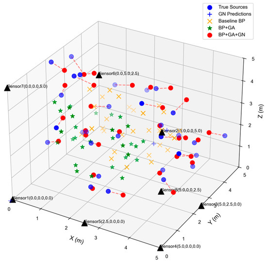
Figure 2.
Comparison of Seismic Source Inversions by Various Algorithms.

Figure 3.
Axis decomposition error.
To provide a more comprehensive quantification and evaluation of the aforementioned characteristics, Figure 4 displays the true source coordinates, predicted coordinates, and error values along each coordinate axis for 15 sample datasets from the axis-wise error experiment. Analysis of the sample results reveals, for instance, that Sample 1 exhibits errors of 0.330 m, −0.110 m, and 0.548 m along the X, Y, and Z axes, respectively, with a total error of 0.649 m. In contrast, Sample 14 demonstrates the highest total error of 0.944 m, while the average errors along the X, Y, and Z axes across all samples are 0.112 m, 0.141 m, and 0.090 m, respectively, resulting in a mean total error of 0.494 m. This value is significantly lower than the average error levels of the BP and BP-GA algorithms. These results statistically validate that the proposed hybrid algorithm achieves superior overall performance in high-precision source localization tasks.
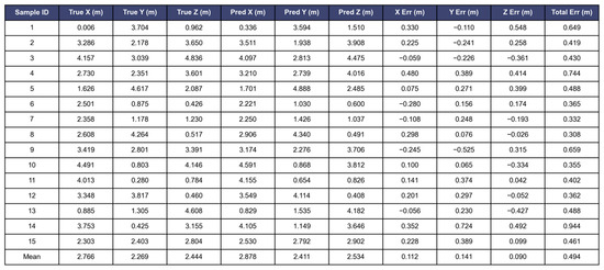
Figure 4.
BP-GA-GN Predicted Values.
From Figure 5 and Figure 6, it can be concluded that the pure GN error distribution has a wide range, with an average error of 17.75 m and a maximum error reaching as high as 87.61 m. Although the BP network reduces the average error to 1.09 m, there is still some degree of scattered error. The BP-GA algorithm, due to the slow convergence and susceptibility to local optima in GA, results in an average error greater than that of the baseline BP network. However, the BP-GA-GN hybrid algorithm, after incorporating GN, achieves an average error of 0.46 m, with the maximum error only 1.25 m, representing improvements of 97.41% and 57.71% compared to GN and BP, respectively.
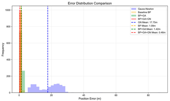
Figure 5.
Error distribution.

Figure 6.
Error statistics.
In the loss and training curves shown in Figure 7, the training loss and validation loss of the BP-GA algorithm are consistently lower than those of the BP network across all training epochs, demonstrating that the BP-GA algorithm has superior training performance. Additionally, the training loss and validation loss curves of the BP-GA algorithm reach stability more quickly, while the BP network exhibits slower convergence. Overall, the BP network with GA incorporated shows better generalization ability, lower risk of overfitting, highlighting the positive impact of GA optimization in improving backpropagation training. In single-sample time difference prediction in Figure 8, the correlation coefficient between the predicted and actual time differences is 0.9906, demonstrating that the algorithm’s output is highly linearly correlated with the real physical quantities, and the model captures the core pattern of the source propagation time difference. Meanwhile, the Mean Squared Error (MSE = 0.00861) and Root Mean Squared Error (RMSE = 0.0941) values are extremely small, confirming that the deviation between the predicted and actual values is controllable, and the algorithm demonstrates high-precision time difference fitting ability in a singlesample scenario. Furthermore, in multi-sample time difference prediction, the real and predicted time difference curves for different samples show a highly consistent overall trend, indicating that the algorithm can stably reproduce the source propagation time difference pattern in multi-sample scenarios. The multi-sample set covers different source locations and sensor combinations, further proving that the algorithm is not reliant on the specific pattern of a single sample but possesses the ability to generalize time difference prediction to multiple scenarios.
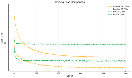
Figure 7.
Training loss curve.
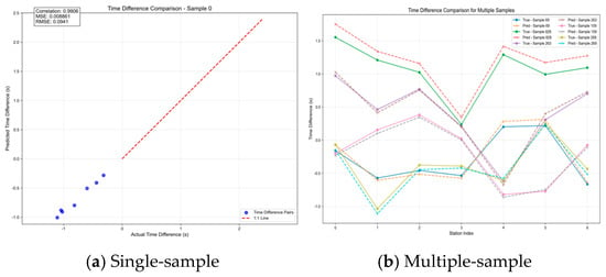
Figure 8.
Sample time difference prediction.
Through experiments simulating geological conditions with normal strata (v = 5 km/s) and a fault zone (v = 3 km/s), as shown in Figure 9, the predicted seismic sources and the actual seismic sources exhibit strong spatial consistency in both the normal geological area (blue) and the fault zone (red). Even within the fault zone, no systematic deviation is observed between the predicted and actual sources, demonstrating the strong robustness of the BP-GA-GN algorithm under geologically heterogeneous conditions.

Figure 9.
Fault Zone Source Inversion Results.
3.2. Mine Example Verification
To validate the applicability of the BP-GA-GN algorithm in engineering applications, microseismic monitoring data from a mining area in western Sichuan Province (primarily consisting of microseismic events induced by drilling and blasting operations, as well as microseismic activities caused by surrounding rock deformation) was selected for testing. The data acquisition was performed using a sampling frequency of 4000 Hz with a 32-bit analog-to-digital converter, 8-channel synchronous acquisition, and dynamic range sampling capabilities. As shown in Figure 10, the monitoring points record the coordinates and time of microseismic events, displaying the daily number of microseismic events in the monitoring area. The pink curve tracks the cumulative number of microseismic events, while the red and orange dots represent deep-hole blasting events and strong microseismic events, respectively. The reliability of the algorithmic model within an actual geological setting was evaluated, yielding the following test results:
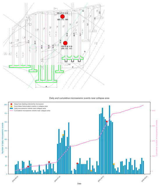
Figure 10.
Mine Microseismic Monitoring Events.
As shown in Figure 11, from the perspective of the spatial distribution of the source points, the prediction results of the GN method show obvious dispersion, especially there is a significant vertical deviation between the Z-axis positive direction region and the real source, reflecting the limitations of a single numerical optimization method under complex geological conditions. The overall positioning accuracy of the BP neural network is limited, and some prediction points have a large offset in the negative direction area of the Y-axis, indicating that the pure data-driven BP model is still insufficient in the extraction and utilization of feature information, and is susceptible to noise interference. After introducing the GA algorithm to optimize the param of the BP neural network, the positioning accuracy has been preliminarily improved, and the predicted points are closer to the real source distribution than the single BP model. This result shows that the global optimization mechanism of GA effectively enhances the convergence performance of BP network and alleviates the problem of falling into local minimum. The BP-GA-GN hybrid algorithm proposed in this paper shows the best positioning performance. Its prediction points are highly consistent with the real source in the whole three-dimensional space, forming a close aggregation distribution, showing the superiority of the three cooperative strategies. The hybrid method significantly improves the robustness and accuracy of source location in complex geological environment. the source points in the mine experimental data, the error distribution characteristics of each axis are shown in Figure 12. In the X-axis direction, the error distribution of the BP network is relatively discrete, and the fluctuation range is roughly between −1.5 m and 0.5 m. The error of BP + GA method is convergent, but there is still a certain degree of dispersion. The error of BP-GA-GN method is concentrated in the narrow range near the zero value, showing better error control ability. The Y-axis error also shows a similar rule: the BP error is dispersed in the range of −1.4 m to 0.2 m, the BP + GA error interval is narrowed, and the error points of BP-GA-GN are closely distributed around the zero value, and the dispersion degree is significantly reduced. In the Z-axis direction, the error of BP network fluctuates greatly, ranging from −2.0 m to 0.0 m. Although the BP + GA method has improved, it is still not ideal. In contrast, the error of the BP-GA-GN method is stably concentrated near the zero value, and the fluctuation range is the smallest. From the comprehensive performance of multi-axis error distribution, BP-GA-GN algorithm shows more robust positioning error control ability in all dimensions.
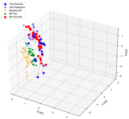
Figure 11.
Comparison of different algorithms for mine seismic source inversion.

Figure 12.
Axis decomposition error.
In order to quantify the statistical significance of the above-mentioned axial error characteristics, Figure 13 lists the three-dimensional real coordinates, predicted coordinates, and detailed data of each axial error and total error of 15 groups of samples. From the perspective of single sample error, the minimum total error of BP-GA-GN method is 0.194 m (sample 3), and the maximum is 0.762 m (sample 2). The total error of most samples is concentrated in the range of 0.2 0.5 m, indicating that the model can achieve medium-precision positioning in most cases. From the statistical mean of each axis, the average errors of X, Y and Z axes are 0.195 m, 0.027 m and 0.031 m, respectively. Among them, the mean error of Z axis is the smallest (absolute value is only 0.031 m), which is consistent with the observation results of the most concentrated error of Z axis in the scatter plot of each axis, which further verifies the stability advantage of the model in the vertical direction. Combined with the scatter plot of the error and the statistical results, it can be seen that the BP-GA-GN algorithm realizes the effective control of the error in the X, Y and Z directions by integrating the global optimization ability of GA and the local correction mechanism of GN.
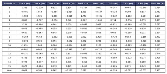
Figure 13.
BP-GA-GN Predicted Values.
As can be observed from Figure 14 and Figure 15, it can be seen that the GN method has the worst performance and the widest error distribution. The high-frequency error is concentrated near 10 m and further away. The mean error is 10.85 m, and the maximum error even reaches 27.69 m. The positioning error is large and unstable. The error of BP network is mainly concentrated in the range of 0 to 5 m, but there is still a certain proportion of median error. The BP neural network model optimized by GA algorithm is 29.51% higher than that of BP, which verifies the effectiveness of GA algorithm in the initialization of BP network weights. The positioning accuracy of the BP-GA-GN hybrid algorithm has been significantly improved. The mean error is 0.42 m, which is 96.17% higher than the GN method and 77.50% higher than the benchmark BP. The maximum error is 1.68 m, which is less than 6% of the GN method. The average error of GN method is 10.85 m, the maximum error is 27.69 m, and the accuracy is the worst. The average error of BP is 1.85 m, which is significantly improved. The average error of BP + GA was 1.30 m, which was 87.99% higher than that of GN method and 29.51% higher than that of BP. The average error of BP-GA-GN is only 0.42 m, the improvement rate of GN method is as high as 96.17%, the improvement rate of BP is 77.50%, and the maximum error is 1.68 m, which is far lower than other algorithms. The accuracy of time difference prediction is the key support for the performance of positioning algorithm. Through two time difference comparison diagrams, the performance of the algorithm in this dimension can be systematically verified. In Figure 13, the predicted time difference and the actual time difference show a high fitting state, the correlation coefficient is as high as 0.9989, the mean square error (MSE) is as low as 0.001859, and the root mean square error (RMSE) is 0.0431. It clearly shows that the algorithm has extremely accurate time difference prediction ability in a single sample scenario, and the deviation between the predicted value and the real value is very small. The verification dimension is further expanded in Figure 16, covering multiple samples such as Sample 15 and 102. It can be seen from the diagram that the predicted time difference curve of different samples is highly consistent with the trend of the real value curve, and the error is always in a controllable range during the change of Station Index. This fully reflects that the algorithm can stably output accurate time difference prediction results in multiple samples and multiple scenarios, laying a data foundation for the improvement of subsequent positioning accuracy, and demonstrating the superiority of the algorithm from the time difference prediction level.
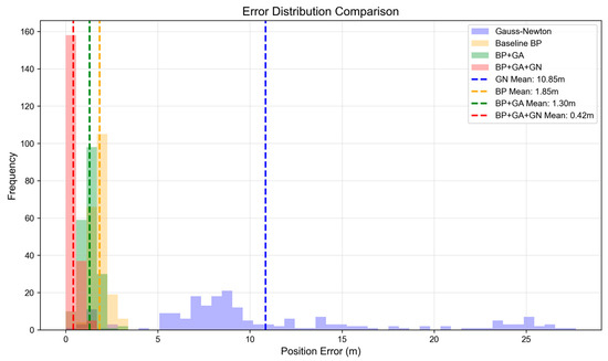
Figure 14.
Error distribution.

Figure 15.
Error statistics.
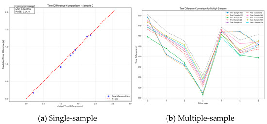
Figure 16.
Sample time difference prediction.
3.3. Tunnel Example Validation
To validate the reliability of the BP-GA-GN algorithm in engineering practice, this study employs microseismic monitoring data from a tunnel in western Sichuan (primarily comprising microseismic events induced by stress redistribution in surrounding rock during tunnel excavation) as a case study. The data acquisition system maintained a sampling frequency of 4000 Hz, equipped with 32-bit analog-to-digital converters, 8-channel synchronous acquisition capability, and dynamic range sampling technology. Through empirical data testing, the algorithm model demonstrated the following reliability characteristics:
As shown in Figure 17, the predicted points obtained by the BP algorithm exhibit a certain similarity to the overall distribution trend of the source points, indicating that the backpropagation algorithm can preliminarily capture the spatial clustering characteristics of the source. However, some points demonstrate an overall translation or rotation, suggesting that the algorithm is prone to getting trapped in local optima under complex tunnel geological conditions. After introducing the GA, the inversion results of the BP-GA algorithm are more globally distributed and closer to the source points, indicating that the GA’s global search mechanism effectively alleviates the BP algorithm’s dependence on initial values, improving the rationality of the inversion results. However, some predicted points still show significant dispersion, particularly in the tunnel boundary areas, suggesting that while the overall structure has improved, local accuracy remains insufficient, possibly due to premature convergence of the GA or parameter setting issues. In contrast, the inversion results of the BP-GA-GN hybrid algorithm proposed in this paper are clearly superior to the previous algorithms. The predicted points not only match the spatial clustering features of the source points but also show excellent localization ability in local areas. Notably, in regions with higher source point density, the BP-GA-GN hybrid algorithm still maintains a low spatial deviation, demonstrating that the GN method, based on BP-GA, further refines the parameter space, effectively converging to a global optimal solution, thereby significantly improving the spatial accuracy and stability of the solution.
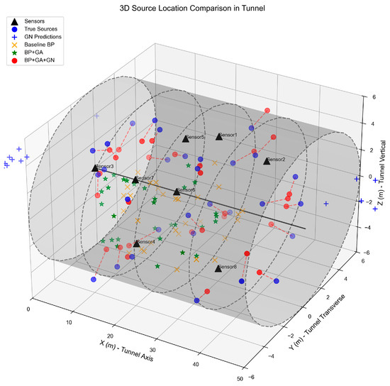
Figure 17.
Comparison of Different Algorithms for Tunnel Seismic Source Inversion.
Figure 18 shows the average errors along the X, Y, and Z axes for different algorithms. The GN method has an error of up to 58.472 m along the X-axis, and although the errors along the other axes are relatively small, the overall performance is poor. The BP algorithm and BP-GA algorithm both show reduced errors compared to the GN method, with improved accuracy. However, the most outstanding result is from the BP-GA-GN hybrid algorithm, where the largest error along the X-axis is only 2.155 m, and the smallest error along the Z-axis is 0.621 m. This balanced low-error level indicates that the BP-GA-GN algorithm not only achieves high overall accuracy but also overcomes anisotropic deviations caused by the model or geometric layout, demonstrating the completeness and robustness of its inversion model.
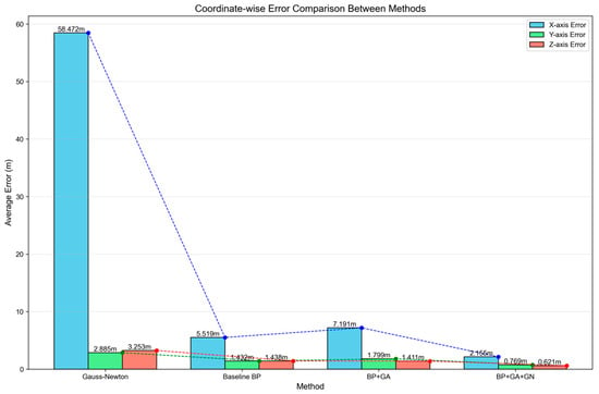
Figure 18.
Comparison of Tunnel Split Axis Errors.
Figure 19 visually reveals the accuracy and stability of the positioning results from different inversion algorithms from a statistical probability perspective. The error distribution curve of the GN method is extremely flat and wide, with the majority of errors falling within the 20 to 100 m range, showing a typical right-skewed distribution characteristic, with the long tail extending towards larger errors. This distribution pattern clearly indicates that the GN method is highly unsuitable for the tunnel seismic source localization problem, with its calculation results being highly unstable, and an average error of 58.73 m. This suggests that the output is almost unusable random noise, unable to effectively converge to the true seismic source. The error distribution of the BP algorithm shows significant improvement, with the distribution narrowing sharply, and the peak appearing within the 0 to 20 m low error range. The majority of events’ errors are controlled within 10 m, and the average error is 6.22 m, proving the basic effectiveness of the BP algorithm in solving such problems. However, there is still a noticeable “tail” on the right side of the distribution, with some events having errors up to 17.13 m, indicating that the algorithm’s performance may degrade significantly in certain locations (such as tunnel boundaries, sensor coverage blind spots) or under specific geological conditions, possibly due to the local minima problem. The error distribution curve of the BP-GA algorithm is similar to that of BP, but its main peak shifts slightly to the left, and the tail becomes heavier. The maximum error increases to 22.67 m, and the average error slightly rises to 7.92 m. This phenomenon reveals the dual-edged nature of GA: its powerful global search ability optimizes the overall solution set to some extent, improving the accuracy of some events. However, its randomness can cause some solutions to deviate from the optimal path, increasing the instability of the inversion results and producing more larger error anomalies. The error distribution of the BP-GA-GN hybrid algorithm presents nearly ideal characteristics: the distribution curve is sharp and highly concentrated in the ultra-low error range of 0–5 m, with the tail being extremely short and quickly decaying to zero. Its average error is only 2.54 m, and the maximum error does not exceed 8.55 m. This distribution feature has an extremely high kurtosis and very low skewness, statistically proving the outstanding performance of the algorithm. It indicates that the hybrid strategy successfully integrates the global exploration capability of GA and the precise local convergence ability of GN, under the good initial framework provided by BP, ultimately achieving extremely high accuracy and stability in the inversion results, effectively eliminating anomalous error points. Furthermore, combining with the data in Figure 20, it can be seen that the average error of the BP-GA-GN algorithm is only 2.54 m, much lower than the 58.73 m of the GN method, 6.22 m of the BP method, and 7.92 m of the BP-GA method. The maximum error is also only 8.55 m, which is significantly smaller than the other algorithms. Compared to the GN method, the accuracy is improved by 95.68%, and relative to the BP network, it shows a 59.15% improvement, strongly demonstrating the excellence of the BP-GA-GN algorithm in error control.

Figure 19.
Tunnel error distribution.

Figure 20.
Tunnel error statistics.
In order to evaluate the stability of BP-GA-GN algorithm in source inversion under noisy conditions, experiments were carried out in scenes without noise and with different noise levels (=0.05, 0.1, 0.2). As shown in Figure 21 and Figure 22, In the noise-free environment (=0), the source points and the algorithm prediction points mainly show significant spatial aggregation, and most of the prediction points are highly coincident with the source points, indicating that BP-GA-GN has high positioning accuracy in an ideal noise-free environment. When introducing low-intensity noise (=0.05), although the noise introduces random disturbances, the spatial offset between the source point and the prediction point is very small. Compared with the noise-free environment, only a few prediction points in the edge area have meter-level deviations due to noise superposition. However, the overall inversion results can still effectively reflect the real spatial distribution characteristics of the source, which preliminarily verifies the algorithm ’s ability to tolerate low-noise interference. In the medium noise (=0.1) environment, the spatial discreteness of the source point and the prediction point increases significantly, but most of the prediction points are still closely around the source point, which still maintains the effectiveness of the source location. In the high-intensity noise (=0.2) environment, the positioning accuracy has decreased, but there is no obvious deviation, and the prediction point is not out of the adjacent area of the source point. Although the inversion accuracy decreases to a certain extent with the increase in noise, the combination of the global search of GA and the local refinement of GN makes the BP-GA-GN algorithm maintain stable positioning performance in noisy environments. Through systematic experimental analysis, it can be concluded that the BP-GA-GN hybrid algorithm shows excellent comprehensive performance in tunnel source location. The algorithm not only significantly improves the positioning accuracy, but also has an average error of only 2.54 m, which is 95.68% and 59.15% lower than the GN method and the BP algorithm, respectively. It also shows a high degree of consistency in spatial distribution, and effectively overcomes the problems of single or partial optimization algorithms that are easy to fall into local minima, sensitive to initial values, and increase errors in the boundary region. More importantly, in the interference experiments with different levels of noise, BP-GA-GN still shows strong robustness and stability, which can resist noise disturbance to a certain extent and maintain credible inversion ability.
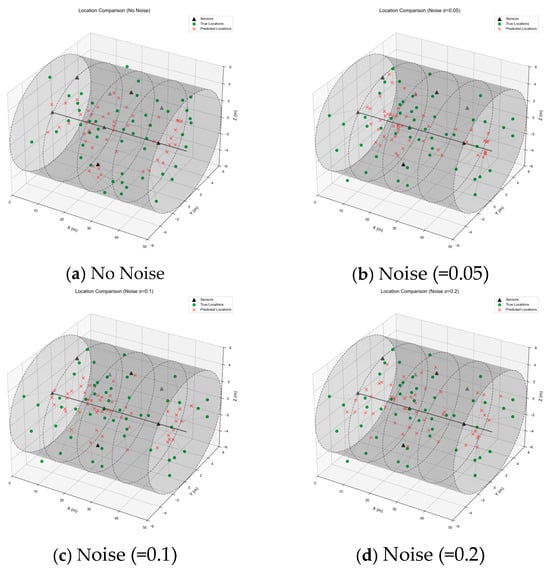
Figure 21.
The inversion results of each noise source.
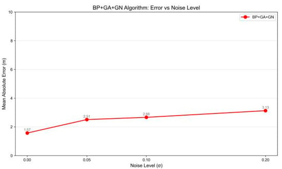
Figure 22.
Algorithm Error Analysis under Different Noises.
4. Conclusions
This paper presents a hybrid optimization algorithm (BP-GA-GN) combining BP neural network (BP), genetic algorithm (GA), and Gauss-Newton method (GN), and conducts experiments using actual microseismic monitoring data from a western mining area in Sichuan and a tunnel in the southwest. Through a multi-angle comparative analysis, the following conclusions are drawn:
- This study proposes a BP-GA-GN hybrid microseismic localization algorithm with a closed-loop collaborative mechanism of “GA global initialization, BP data-driven fitting, GN physical constraint refinement”, which fundamentally breaks through the limitations of existing hybrid algorithms that rely on “pairwise splicing”. Specifically, GA optimizes BP’s initial parameters to avoid local optima, BP learns the nonlinear mapping between sensor time differences and source positions, and GN realizes fine convergence based on the physical model of seismic wave propagation—jointly ensuring the algorithm’s balance of global search capability and local optimization precision.
- The BP-GA-GN fusion algorithm adopts a deep integration of physical models and data-driven approaches. By relying on the physical geometric model of seismic wave propagation, it constrains and refines the learning results of the BP network, bridging the gap between pure data-driven “black-box” models and physical laws to some extent. This mechanism not only enhances the physical interpretability and reliability of the localization results but also accelerates convergence speed, overcoming the accuracy stagnation problem that may occur during BP network training.
- Tests of the BP-GA-GN fusion algorithm in the actual scenarios of a complex mining area in the southwest and a tunnel in the southwest, achieving average errors of 0.42 m and 2.54 m, respectively. These results demonstrate that the BP-GA-GN algorithm maintains good localization performance under different geological conditions. In terms of sensor time difference prediction, the correlation coefficients between simulated and measured data are 0.9906 and 0.9989, respectively, with both MSE and RMSE remaining at low levels. The prediction curves show good alignment across different sample and sensor combinations, indicating strong generalization. In the future, we will compare the BP-GA-GN algorithm with common hybrid algorithms in more complex geological environments to further test its accuracy and robustness.
Author Contributions
Resources, N.Y.; Writing—original draft, Y.W.; Project administration, S.Z. All authors have read and agreed to the published version of the manuscript.
Funding
Research on Integrated Technology of Microseismic Monitoring and Rockburst Early Warning for Deep Buried High Geostress Tunnels of China State Railway Group Project (KSNQ243013).
Institutional Review Board Statement
Not applicable.
Informed Consent Statement
Not applicable.
Data Availability Statement
The data presented in this study are available on request from the corresponding author.
Conflicts of Interest
Author Siwei Zhao was employed by the company China Railway Eryuan Engineering Group Co. The authors declare that this study received funding from China State Railway Group. The funder was not involved in the study design, collection, analysis, interpretation of data, the writing of this article or the decision to submit it for publication. The remaining authors declare that the research was conducted in the absence of any commercial or financial relationships that could be construed as a potential conflict of interest.
References
- Feng, X.T.; Chen, B.R.; Zhang, C.Q.; Li, S.J.; Wu, S.Y. Mechanism, Early Warning and Dynamic Control of Rockburst Evolution Process; Science Press: Beijing, China, 2003. [Google Scholar]
- Geiger, L. Probability method for the determination of earthquake epicenters from the arrival time only. Bull. St. Louis Univ. 1912, 8, 60–71. [Google Scholar]
- Lee, W.H.K.; Lahr, J.C. HYPO71: A Computer Program for Determining Hypocenter, Magnitude, and First Motion Pattern of Local Earthquakes; US Department of the Interior, Geological Survey, National Center for Earthquake Research: Golden, CO, USA, 1972.
- Klein, F.W. Hypocenter Location Program HYPOINVERSE: Part I. Users Guide to Versions 1, 2, 3, and 4. Part II. Source Listings and Notes; US Geological Survey: Reston, VA, USA, 1978.
- Lienert, B.R.; Berg, E.; Frazer, L.N. HYPOCENTER: An earthquake location method using centered, scaled, and adaptively damped least squares. Bull. Seismol. Soc. Am. 1986, 76, 771–783. [Google Scholar] [CrossRef]
- Nelson, G.D.; Vidale, J.E. Earthquake locations by 3-D finite-difference travel times. Bull. Seismol. Soc. Am. 1990, 80, 395–410. [Google Scholar] [CrossRef]
- Zhao, Z.; Ding, Z.F.; Yi, G.X.; Wang, J.G. Tibet Earthquake Localization—A Nonlinear Method Using Simplex Optimization. Acta Seismol. Sin. 1994, 16, 212–219. [Google Scholar]
- Wei, C.; Li, X.F.; Zheng, X.D. Parallel Algorithm for Serial Monte Carlo Inversion Method Based on Population Search. Appl. Geophys. 2010, 7, 127–134+193. [Google Scholar] [CrossRef]
- Zhu, W.X.; Zhang, X.C.; Zhang, W.B.; Wang, Z.H.; Tian, Z.C. Seismic Data Spectrum Inversion Technology Based on Simulated Annealing Algorithm. Pet. Geophys. Prospect. 2015, 50, 495–501+515. [Google Scholar]
- Sambridge, M.; Drijkoningen, G. Genetic algorithms in seismic waveform inversion. Geophys. J. Int. 1992, 109, 323–342. [Google Scholar] [CrossRef]
- Zhao, H.B.; Liu, R.; Gu, T.; Liu, Y.H.; Jiang, D.M. Research on Automatic P-Wave Picking Method for Microseismic Signals Based on Deep Learning Model. J. Rock Mech. Eng. 2021, 40, 3084–3097. [Google Scholar]
- Zhang, X.; Zhang, J.; Yuan, C.; Liu, S.; Chen, Z.; Li, W. Locating induced earthquakes with a network of seismic stations in Oklahoma via a deep learning method. Sci. Rep. 2020, 10, 1941. [Google Scholar] [CrossRef] [PubMed]
- Tao, C.H.; He, Q.D.; Wang, X.C. Inversion of Layered Elastic Media Using Genetic Algorithm. Pet. Geophys. Prospect. 1994, 29, 382–386. [Google Scholar]
- Cary, P.W.; Chapmann, C.H. Automatic 1-D waveform inversion of marine seismic refraction data. Geophys. J. Int. 1988, 93, 527–546. [Google Scholar] [CrossRef]
- Raghu, K.C.; Mrinal, K.S.; Paul, L.S. Hybrid optimization methods for geophysical inversion. Geophysics 1997, 62, 1196–1207. [Google Scholar] [CrossRef]
- Carlos, C.-M.; Mrinal, K.S.; Paul, L.S. Artificial neural networks for parameter estimation in geophysics. Geophys. Prospect. 2000, 48, 28–47. [Google Scholar] [CrossRef]
- Stork, C.; Kusuma, T. Hybrid genetic auto static: New approach for largeamplitude statics with noisy data. Geophysics 1992, 1992, 1127–1131. [Google Scholar]
- Zhang, L.B.; Yao, Z.X. Hybrid Optimization Method for Parameter Inversion of Layered Media. Adv. Geophys. 2000, 15, 46–53. [Google Scholar] [CrossRef]
- Wang, L.F. Research on the Localization Technology of Microseismic Source Points for Oil Well Fracturing Based on Genetic Algorithm. Ph.D. Thesis, College of Instrumentation Science and Electrical Engineering, Jilin University, Changchun, China, 2012. [Google Scholar]
- Han, Y.N. Research on Coal Seam Microseismic Localization System Based on GA-PSO Hybrid Algorithm. Master’s Thesis, Jilin University, Changchun, China, 2025. [Google Scholar] [CrossRef]
- Zhou, G.Q.; Luo, S.L.; Gao, Y.X.; Zhang, W.; Jin, X.; Meng, F.; Wang, Y. Research on GA-PSO Microseismic Source Location Optimization Algorithm Based on Hierarchical Structure and Multi-Strategy Adaptive Mechanism. Coal Science and Technology, 1–12 [25 November 2025]. Available online: https://link.cnki.net/urlid/11.2402.TD.20250825.1256.004 (accessed on 23 November 2025).
- Liao, Z.; Feng, T.; Yu, W.J.; Cui, D.J.; Wu, G.S. Microseismic Source Location Method and Application Based on NM-PSO Algorithm. Appl. Sci. 2022, 12, 8796. [Google Scholar] [CrossRef]
Disclaimer/Publisher’s Note: The statements, opinions and data contained in all publications are solely those of the individual author(s) and contributor(s) and not of MDPI and/or the editor(s). MDPI and/or the editor(s) disclaim responsibility for any injury to people or property resulting from any ideas, methods, instructions or products referred to in the content. |
© 2025 by the authors. Licensee MDPI, Basel, Switzerland. This article is an open access article distributed under the terms and conditions of the Creative Commons Attribution (CC BY) license (https://creativecommons.org/licenses/by/4.0/).