Tensorized Consensus Graph Learning for Incomplete Multi-View Clustering with Confidence Integration

Abstract

Graph-based multi-view clustering has gained significant attention in recent years due to its superior ability to reveal clustering structures. However, existing methods often incur high computational costs when capturing local information and overlook the higher-order correlations between multiple views. To address these issues, we propose Tensorized Consensus Graph Learning for Incomplete Multi-View Clustering with Confidence Integration (TCGL). This approach constructs adjacency and local heat kernel graphs by filtering missing samples to better capture local structures while leveraging a t-SVD-based weighted tensor nuclear norm sparsification method to reduce noise. Additionally, we introduce a matrix energy-based adjacency graph normalization strategy that utilizes common nearest neighbors to generate probability matrices, enhancing noise resistance and improving structural exploration. Experimental results demonstrate that TCGL effectively handles incomplete data and significantly outperforms state-of-the-art approaches across multiple datasets.

1. Introduction

Multi-view clustering (MVC) is a technique that enhances clustering performance by integrating data from multiple sources or feature representations, allowing for a more comprehensive understanding of complex objects [1]. Real-world entities, such as images, users or biological samples, can usually be described from multiple complementary perspectives [2]. For instance, an image may be represented using a variety of descriptors including color histograms, textural patterns, and shape descriptors [3], while a user’s profile might encompass multi-faceted information [4], such as social connections [5], behavior logs and text content [6]. The objective of MVC is to leverage the complementarity and consistency between these views and thereby more accurately capture the intrinsic data structure.

In practical applications, multi-view data frequently encounters a range of challenges [7], such as missing instances caused by sensor failures or data corruption, noise interference, and the inherent difficulty of aligning heterogeneous data sources [8]. Consequently, Incomplete Multi-view Clustering (IMVC) algorithms have been devised to address these issues [9]. Current IMVC methods can be generally divided into two principal categories [10]. The first approach relies on graph-based techniques [11], where a similarity graph is constructed for each view, and clustering is subsequently achieved by leveraging the spectral properties of the graph Laplacian matrix [12]. For example, Liu et al. [13] presented an efficient incomplete multi-view clustering method (EE-IMVC) that iteratively refines the base clustering matrix and the consensus clustering matrix to enhance clustering outcomes. Additionally, Wen et al. [14] proposed a consensus graph learning framework grounded in high-confidence local structures (HCLS-CGL), which enhances noise robustness by learning cross-view consensus graphs and incorporating confidence graph constraints. The second approach employs non-negative matrix factorization (NMF) method for multi-view clustering task [15], which uncovers latent data structures by decomposing the data matrix into two or more non-negative factor matrices. Within this paradigm, Khan et al. [16] put forward the Manifold Regularized Multi-view Fuzzy Clustering Method (MRFCM). This approach maintains the innate geometric configuration of the data through manifold regularization and dimension reduction, while simultaneously mitigating overfitting and enhancing sparsity through a combined use of the Frobenius norm and L1-norm. Furthermore, Luong et al. [17] introduced a deep non-negative matrix factorization-based multi-view clustering approach (ODD-NMF), which preserves the structural relationships within the data through multi-layer manifold learning, integrating diversity and orthogonality constraints to optimize clustering performance.

However, existing methods still have several limitations [18]. Many methods are limited to dual-view data or necessitate the completeness of at least one view. Additionally, learning graph structures directly from raw data can easily introduce a large amount of noise [14]. For instance, Gaussian-kernel-based graphs lack universal applicability, and the self-expressive property of original data is especially sensitive to anomalous points [19]. Furthermore, most methods focus on common representations or pairwise view relationships, inadequately capturing the higher-order interdependencies within multi-view data and consequently resulting in the loss of vital underlying semantic information [20]. Compounding these issues, the graph learning process in most methods is typically disconnected from the clustering objective [21], as prior knowledge about the desired cluster structure is rarely incorporated. This disjunction ultimately results in severely suboptimal performance.

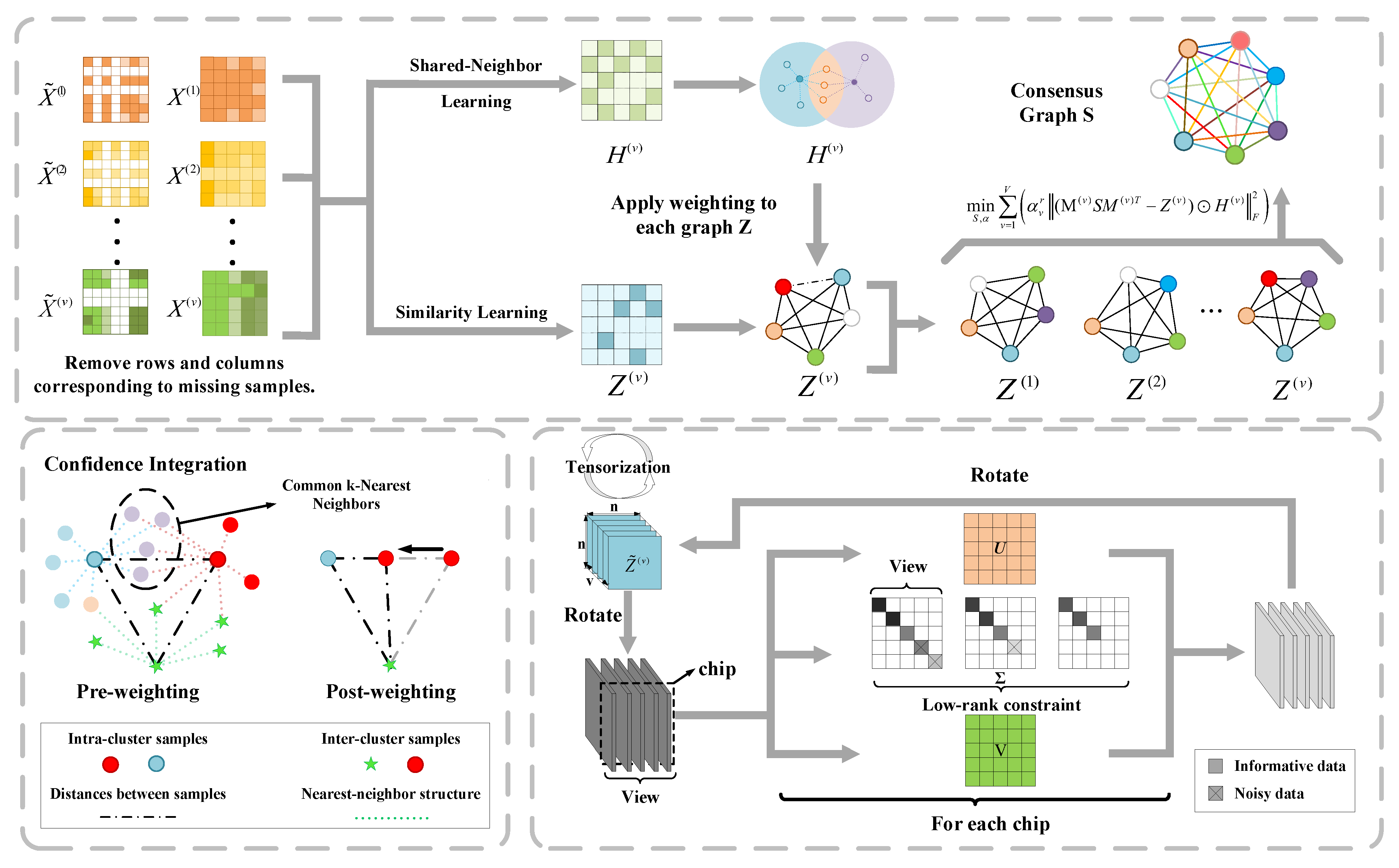
To tackle these challenges, we propose a novel method termed Tensorized Consensus Graph Learning (TCGL) for incomplete multi-view clustering. As illustrated in Figure 1, TCGL constructs adjacency graphs and local heat kernel graphs by filtering missing samples and retaining valid data, which aids in representing the data’s local structural characteristics. To this end, the local heat kernel matrices are assembled into a tensor. We then employ a weighted tensor nuclear norm minimization, grounded in t-SVD, to denoise the constructed tensor and preserve critical similarity structures that are often obscured in graphs derived directly from raw data. Furthermore, the adjacency graph of each view is normalized by its matrix energy to enhance multi-view consistency and clustering performance. Subsequently, the sparsified local heat kernel graphs and the probability matrices are fused into a consensus graph, which more accurately captures the underlying data structures across all views. The major contributions of this paper are summarized as follows:

Figure 1. Illustration of the proposed TCGL model. Given an incomplete multi-view dataset $\mathbf{X}$, TCGL first processes the incomplete data to construct the adjacency graph ${\mathbf{H}}^{\left(\mathbf{v}\right)}$ and the local heat kernel graph ${\mathbf{Z}}^{\left(\mathbf{v}\right)}$. The heat kernel matrices are then assembled into a tensor and refined by a t-SVD-based sparsification module to enhance high-similarity information and reduce noise. Concurrently, the adjacency graph ${\mathbf{H}}^{\left(\mathbf{v}\right)}$ is normalized to generate a probability matrix. Finally, these components are fused to learn a consensus graph for multi-view clustering.

• We propose the Tensorized Consensus Graph Learning (TCGL) with a confidence integration framework for incomplete multi-view clustering, which leverages missing sample filtration to construct adjacency and local heat kernel graphs, thereby enhancing the preservation of local structural information.
• A probability matrix generation strategy based on common nearest neighbors is employed, coupled with a t-SVD-based weighted tensor nuclear norm sparsification technique. This integration effectively mitigates noise, retains high-value similarity information, and strengthens structural representation learning.
• TCGL framework is optimized with an alternating minimization algorithm. Extensive evaluations on several benchmark datasets validate that our approach surpasses existing state-of-the-art IMVC techniques.

This paper is structured as follows. Section 2 covers the preliminaries. Section 3 elaborates on the proposed TCGL method, followed by the description of the optimization algorithm in Section 4. Section 5 evaluates the experimental results, and Section 6 provides the concluding remarks and future work.

2. Preliminary

This section presents the notation and key preliminaries that form the foundation for our proposed method, is cataloged in Table 1. The input is an incomplete multi-view dataset $\mathbf{X}=\{{\mathbf{X}}^{\left(1\right)},{\mathbf{X}}^{\left(2\right)},\dots ,{\mathbf{X}}^{\left(v\right)}\}$, where ${\mathbf{X}}^{\left(v\right)}\in {\mathbb{R}}^{d_v\times n}$ denotes the feature matrix of the v-th view ($v=1,2,\dots ,V$). Here, $d_v$ represents the feature dimensionality of the v-th view, n is the total number of samples across all views, and each column ${{\mathbf{X}}^{\left(\mathbf{v}\right)}}_{:,i}\in {\mathbb{R}}^{d_v}$ ($i=1,2,\dots ,n$) corresponds to the feature representation of the i-th sample in the v-th view.

2.1. Notation

2.1.1. Basic Symbol Conventions

• Calligraphic letters (e.g., $\mathcal{A},\mathcal{X}$) represent tensors (typically 3D tensors for multi-view graph modeling in this work);
• Bold uppercase letters (e.g., $\mathbf{A},{\mathbf{X}}^{\left(v\right)}$) denote matrices;
• Bold lowercase letters (e.g., $\mathbf{a},{\mathbf{x}}_i^{\left(v\right)}$) signify vectors;
• Plain lowercase letters (e.g., $n,d_v,V$) represent scalars (e.g., sample count, feature dimensionality, view number).

For a matrix $\mathbf{A}\in {\mathbb{R}}^{m\times n}$:

• ${\mathbf{A}}_{:,i}$ denotes the i-th column vector of $\mathbf{A}$;
• ${\mathbf{A}}_{i,:}$ denotes the i-th row vector of $\mathbf{A}$;
• ${\mathbf{A}}_{i,j}$ denotes the element at the i-th row and j-th column of $\mathbf{A}$;
• $\left|\mathbf{A}\right|$ denotes the element-wise absolute value operation (i.e., ${\left|\mathbf{A}\right|}_{i,j}=\left|{\mathbf{A}}_{i,j}\right|$);
• $\mathbf{A}\ge 0$ indicates that all elements of $\mathbf{A}$ are non-negative;
• $\mathrm{rank}\left(\mathbf{A}\right)$ denotes the rank of $\mathbf{A}$;
• ${\mathbf{1}}_{m\times n}$ and ${\mathbf{1}}_n$ are the compact notation for an all-ones matrix and an n-dimensional all-ones vector, respectively (with dimensions omitted when evident).

Table 1. List of matrix, tensor and set symbols.

Symbol	Dimension	Description
$\mathbf{X}$	set	Incomplete multi-view dataset $\{X^{\left(1\right)},\dots ,X^{\left(V\right)}\}$
${\mathbf{X}}^{\left(\mathbf{v}\right)}$	${\mathbb{R}}^{d_v\times n}$	Feature matrix of view v
$\mathbf{O}$	${\mathbb{R}}^{n\times V}$	Missing-indicator matrix
${\mathbf{M}}^{\left(\mathbf{v}\right)}$	${\mathbb{R}}^{n\times n}$	Diagonal mask for available samples in view v
${\tilde{\mathbf{Z}}}^{\left(\mathbf{v}\right)}$	${\mathbb{R}}^{n_v\times n_v}$	Local similarity between available samples in view v
${\mathbf{Z}}^{\left(\mathbf{v}\right)}$	${\mathbb{R}}^{n\times n}$	Full similarity graph of view v (zero-padded)
${\tilde{\mathbf{H}}}^{\left(v\right)}$	${\mathbb{R}}^{n_v\times n_v}$	Co-neighbor probability in view v
${\mathbf{H}}^{\left(\mathbf{v}\right)}$	${\mathbb{R}}^{n\times n}$	Full co-neighbor confidence graph of view v
$\mathbf{S}$	${\mathbb{R}}^{n\times n}$	Consensus similarity graph for clustering
${\mathbf{L}}_{\mathbf{S}}$	${\mathbb{R}}^{n\times n}$	Normalized Laplacian of consensus graph S
$\mathcal{Z}$	${\mathbb{R}}^{n\times n\times V}$	Tensor stacking all $Z^{\left(v\right)}$ graphs
$\mathcal{J}$	${\mathbb{R}}^{n\times n\times V}$	Auxiliary tensor for low-rank regularization
$\mathcal{Q}$	${\mathbb{R}}^{n\times n\times V}$	Lagrange-multiplier tensor in ALM
$\alpha$	${\mathbb{R}}^V$	View-weight vector ${[{\alpha }_1,\dots ,{\alpha }_V]}^T$
$\omega$	${\mathbb{R}}^{min(n,V)}$	Weight vector for tensor nuclear norm shrinkage
$\mathbf{F}$	${\mathbb{R}}^{n\times c}$	Spectral embedding matrix

Table 1. List of matrix, tensor and set symbols.

Symbol	Dimension	Description
$\mathbf{X}$	set	Incomplete multi-view dataset $\{X^{\left(1\right)},\dots ,X^{\left(V\right)}\}$
${\mathbf{X}}^{\left(\mathbf{v}\right)}$	${\mathbb{R}}^{d_v\times n}$	Feature matrix of view v
$\mathbf{O}$	${\mathbb{R}}^{n\times V}$	Missing-indicator matrix
${\mathbf{M}}^{\left(\mathbf{v}\right)}$	${\mathbb{R}}^{n\times n}$	Diagonal mask for available samples in view v
${\tilde{\mathbf{Z}}}^{\left(\mathbf{v}\right)}$	${\mathbb{R}}^{n_v\times n_v}$	Local similarity between available samples in view v
${\mathbf{Z}}^{\left(\mathbf{v}\right)}$	${\mathbb{R}}^{n\times n}$	Full similarity graph of view v (zero-padded)
${\tilde{\mathbf{H}}}^{\left(v\right)}$	${\mathbb{R}}^{n_v\times n_v}$	Co-neighbor probability in view v
${\mathbf{H}}^{\left(\mathbf{v}\right)}$	${\mathbb{R}}^{n\times n}$	Full co-neighbor confidence graph of view v
$\mathbf{S}$	${\mathbb{R}}^{n\times n}$	Consensus similarity graph for clustering
${\mathbf{L}}_{\mathbf{S}}$	${\mathbb{R}}^{n\times n}$	Normalized Laplacian of consensus graph S
$\mathcal{Z}$	${\mathbb{R}}^{n\times n\times V}$	Tensor stacking all $Z^{\left(v\right)}$ graphs
$\mathcal{J}$	${\mathbb{R}}^{n\times n\times V}$	Auxiliary tensor for low-rank regularization
$\mathcal{Q}$	${\mathbb{R}}^{n\times n\times V}$	Lagrange-multiplier tensor in ALM
$\alpha$	${\mathbb{R}}^V$	View-weight vector ${[{\alpha }_1,\dots ,{\alpha }_V]}^T$
$\omega$	${\mathbb{R}}^{min(n,V)}$	Weight vector for tensor nuclear norm shrinkage
$\mathbf{F}$	${\mathbb{R}}^{n\times c}$	Spectral embedding matrix

2.1.2. Graph Laplacian Matrix

For a similarity matrix $\mathbf{B}\in {\mathbb{R}}^{n\times n}$ (constructed to describe sample similarity in a single view), its symmetric normalized graph Laplacian is defined as:

$${\mathbf{L}}_{\mathbf{B}}={\mathbf{D}}_{\mathbf{B}}-{\displaystyle \frac{\left|\mathbf{B}\right|+{\left|\mathbf{B}\right|}^T}{2}},$$

(1)

where ${\mathbf{D}}_{\mathbf{B}}\in {\mathbb{R}}^{n\times n}$ is the degree matrix corresponding to $\mathbf{B}$, and its i-th diagonal element is calculated as:

$${\left({\mathbf{D}}_{\mathbf{B}}\right)}_{i,i}={\displaystyle \sum _{j=1}^n}{\displaystyle \frac{|{\mathbf{B}}_{i,j}|+|{\mathbf{B}}_{j,i}|}{2}}.$$

(2)

2.1.3. Tensor-Related Operations

For a 3D tensor $\mathcal{A}\in {\mathbb{R}}^{m\times n\times k}$ (used to stack k view-specific similarity matrices in this work):

• ${\mathcal{A}}^{\left(t\right)}\in {\mathbb{R}}^{m\times n}$ denotes the t-th frontal slice of $\mathcal{A}$ (i.e., the matrix obtained by fixing the third dimension at index t, $t=1,2,\dots ,k$);
• Fast Fourier Transform (FFT) along the third dimension: $\overline{\mathcal{A}}=\mathrm{fft}(\mathcal{A},\left[\right],3)$, where ${\overline{\mathcal{A}}}^{\left(t\right)}$ is the FFT result of the t-th frontal slice;
• Inverse FFT (IFFT) recovery: $\mathcal{A}=\mathrm{ifft}(\overline{\mathcal{A}},\left[\right],3)$, which reconstructs the original tensor from its frequency-domain representation $\overline{\mathcal{A}}$;

2.1.4. Block Vectorization

Converts a 3D tensor into a 2D matrix by concatenating its frontal slices vertically, defined as:

$$\mathrm{bvec}\left(\mathcal{A}\right)=\left[\begin{array}{c}{\mathcal{A}}^{\left(1\right)}\\ {\mathcal{A}}^{\left(2\right)}\\ ⋮\\ {\mathcal{A}}^{\left(k\right)}\end{array}\right]\in {\mathbb{R}}^{mk\times n}.$$

(3)

The inverse operation (block folding) recovers the tensor from its block-vectorized form: $\mathrm{bvfold}\left(\mathrm{bvec}\right(\mathcal{A}\left)\right)=\mathcal{A}$.

2.1.5. Block Circulant Matrix

Constructed from the frontal slices of $\mathcal{A}$ to enable tensor singular value decomposition (t-SVD) via matrix operations, defined as:

$$\mathrm{bcirc}\left(\mathcal{A}\right)=\left[\begin{array}{ccccc}{\mathcal{A}}^{\left(1\right)}& {\mathcal{A}}^{\left(k\right)}& {\mathcal{A}}^{(k-1)}& \dots & {\mathcal{A}}^{\left(2\right)}\\ {\mathcal{A}}^{\left(2\right)}& {\mathcal{A}}^{\left(1\right)}& {\mathcal{A}}^{\left(k\right)}& \dots & {\mathcal{A}}^{\left(3\right)}\\ ⋮& ⋮& ⋮& \ddots & ⋮\\ {\mathcal{A}}^{\left(k\right)}& {\mathcal{A}}^{(k-1)}& {\mathcal{A}}^{(k-2)}& \dots & {\mathcal{A}}^{\left(1\right)}\end{array}\right]\in {\mathbb{R}}^{mk\times nk}.$$

(4)

This structure ensures that the t-SVD of $\mathcal{A}$ is equivalent to the conventional SVD of $\mathrm{bcirc}\left(\mathcal{A}\right)$ in the frequency domain, which simplifies the optimization of tensor nuclear norm regularization.

Definition 1

(Transpose of a Tensor [22]). For a tensor $\mathcal{A}\in {\mathbb{R}}^{n_1\times n_2\times n_3}$, its transpose ${\mathcal{A}}^T\in {\mathbb{R}}^{n_2\times n_1\times n_3}$ is acquired by initially transposing each frontal slice ($A^{\left(k\right)}$) and subsequently reversing the sequence of the transposed slices from 2 to $n_3$.

Definition 2

(Identity Tensor). The identity tensor $\mathcal{I}$ is an $n_1\times n_1\times n_3$ tensor, characterized by an identity matrix of size $n_1\times n_1$ as its first frontal slice, with all other frontal slices being null.

Definition 3

(Orthogonal Tensor). A tensor $\mathcal{A}$ is deemed orthogonal if it satisfies the conditions ${\mathcal{A}}^T·\mathcal{A}=\mathcal{A}·{\mathcal{A}}^T=\mathcal{I}$.

Definition 4

(t-Product). For tensors $\mathcal{A}\in {\mathbb{R}}^{n_1\times n_2\times n_3}$ and $\mathcal{B}\in {\mathbb{R}}^{n_2\times n_4\times n_3}$, their t-product $\mathcal{A}·\mathcal{B}$ results in a tensor $\mathcal{E}$ of dimensions $n_1\times n_4\times n_3$, defined as follows:

$$\begin{array}{c}\hfill \mathcal{E}=\mathcal{A}\ast \mathcal{B}=\mathrm{bvfold}\left(\mathrm{bcirc}\right(\mathcal{A})\ast \mathrm{bvec}(\mathcal{B}\left)\right).\end{array}$$

(5)

The t-product between $\mathcal{A}$ and $\mathcal{B}$ can be swiftly computed by multiplying corresponding frontal slices in the Fourier domain:

$$\begin{array}{c}{\overline{\mathbf{E}}}^{\left(k\right)}={\overline{\mathbf{A}}}^{\left(k\right)}\ast {\overline{\mathbf{B}}}^{\left(k\right)},k=1,\dots ,n_3,\hfill \end{array}$$

(6)

and then obtaining the t-product $\mathcal{E}=\mathrm{ifft}(\mathcal{E};[2,3\left]\right)$.

Definition 5

(t-SVD [23]). A tensor $\mathcal{A}\in {\mathbb{R}}^{n_1\times n_2\times n_3}$ can be factorized via its t-SVD as:

$$\begin{array}{c}\mathcal{A}=\mathcal{U}\ast \mathcal{S}\ast {\mathcal{V}}^T,\end{array}$$

(7)

where $\mathcal{U}\in {\mathbb{R}}^{n_1\times n_1\times n_3}$ and $\mathcal{V}\in {\mathbb{R}}^{n_2\times n_2\times n_3}$ are orthogonal tensors, and $\mathcal{S}\in {\mathbb{R}}^{n_1\times n_2\times n_3}$ is an f-diagonal tensor with diagonal matrices as its frontal slices.

Following [23], an efficient computation of the t-SVD leverages the matrix SVD within the Fourier domain.

$${\overline{\mathbf{A}}}^{\left(k\right)}={\overline{\mathbf{U}}}^{\left(k\right)}{\overline{\mathbf{S}}}^{\left(k\right)}{\left({\overline{\mathbf{V}}}^{\left(k\right)}\right)}^T,k=1,\dots ,n_3.$$

(8)

Definition 6

(Tensor Multi-Rank). For a tensor $\mathcal{A}\in {\mathbb{R}}^{n_1\times n_2\times n_3}$, its multi-rank is defined as a vector $\mathbf{r}\in {\mathbb{R}}^{n_3\times 1}$, where the i-th element corresponds to the rank of the i-th frontal slice of $\mathcal{A}$.

Definition 7

(t-SVD Based Tensor Nuclear Norm [24]). Given a tensor $\mathcal{A}\in {\mathbb{R}}^{n_1\times n_2\times n_3}$, its t-SVD based tensor nuclear norm (t-TNN) is expressed as:

$${\parallel \mathcal{A}\parallel }_{⊛}={\displaystyle \sum _{k=1}^{n_3}}{\parallel {\mathbf{A}}^{\left(\mathbf{k}\right)}\parallel }_{\ast }={\displaystyle \sum _{k=1}^{n_3}}{\displaystyle \sum _{i=1}^{min(n_1,n_2)}}{\sigma }_i\left({\mathbf{A}}^{\left(\mathbf{k}\right)}\right),$$

(9)

where ${\sigma }_i\left({\mathbf{A}}^{\left(\mathbf{k}\right)}\right)$ denotes the i-th largest singular value of $A^{\left(k\right)}$.

Additionally, the weighted t-SVD based tensor nuclear norm is defined as:

$${\parallel \mathcal{A}\parallel }_{\omega ,⊛}={\displaystyle \sum _{k=1}^{n_3}}{\displaystyle \sum _{i=1}^{min(n_1,n_2)}}{w}_i{\sigma }_i\left({\mathbf{A}}^{\left(\mathbf{k}\right)}\right),$$

(10)

where $w_i$ is the weight associated with ${\sigma }_i\left({\mathbf{A}}^{\left(k\right)}\right)$, allowing the incorporation of prior knowledge regarding the singular values of the matrices.

Remark 1.

In this work, the weight vector $\omega =[w_1,...,w_i]$ is initialized uniformly as $w_i=1/min(n_1,n_2)$ for $i=1,\dots ,min(n_1,n_2)$, ensuring equal contribution from all singular value components at the start of optimization. Furthermore, ω remains fixed throughout the learning process. This design provides a stable regularization framework. The model’s adaptability to the importance of different views is primarily handled through the optimization of the view-weighting vector α and the low-rank constraints on the tensor slices.

3. The Proposed Method

We present a graph-based consensus learning framework for incomplete multi-view clustering. TCGL comprises three key stages: addressing missing data, constructing KNN binary and confidence graphs, and consolidating the confidence graphs into a tensor for low-rank processing. The weighted confidence graph facilitates the generation of a consensus graph, which is subsequently clustered using K-means.

The existing approaches for dealing with incomplete data, such as imputation, distance-based adjustment [25], weighted processing, latent model inference, and dimensionality reduction, are all subject to limitations. These limitations include introducing biases, escalating computational costs, losing information, and depending on subjective rules. To overcome these challenges, TCGL strategically excludes the dimensions containing missing values for each sample through the constructed index matrix. By constructing a location index matrix $\mathbf{O}\in {\{0,1\}}^{n\times l}$, where ${\mathbf{O}}_{i,j}=1$ indicates the j-th view of the i-th sample is not missing, and ${\mathbf{O}}_{i,j}=0$ indicates it is missing. ${\mathbf{M}}_{i,j}^{\left(v\right)}$ is constructed by the prior location indices $\mathbf{O}$ for filtering complete data and aligning data, as follows:

$${\mathbf{M}}_{i,j}^{\left(v\right)}=\left\{\begin{array}{cc}1,\hfill & ifthej-thsamlpehasanavailable\hfill \\ \hfill & instance{x}_i^{\left(v\right)}inthev-thview\hfill \\ 0,\hfill & otherwise.\hfill \end{array}\right.$$

(11)

Consensus Graph Learning Method

The standard procedure for graph-based spectral clustering [26,27] includes three key steps: affinity graph construction, eigen-decomposition of the graph Laplacian matrix, and final cluster assignment via k-means. The affinity graph is an $n\times n$ matrix, where n represents the number of samples in the data, and the elements of the matrix indicate the relationships between the samples, such as their similarity or distance. Among these steps, the construction of the affinity graph is particularly important as it significantly impacts the final clustering results.

In recent years, several methods for constructing high-quality affinity graphs have been proposed [28,29,30] aiming to better capture the intrinsic relationships between the data points. One such method is the constrained Laplacian rank (CLR) approach [31]. CLR aims to learn a new similarity matrix that reflects the cluster structure by ensuring that the matrix has exactly c blocks, each corresponding to one of the c clusters. The formulation of this problem is as follows:

$$\begin{array}{c}\underset{\mathbf{S}}{min}{\parallel \mathbf{S}-\mathbf{G}\parallel }_F^2,\\ \mathrm{s}.\mathrm{t}.0\le \mathbf{S}\le 1,\mathbf{S}\mathbf{1}=\mathbf{1},\mathrm{rank}\left({\mathbf{L}}_{\mathbf{S}}\right)=n-c,\mathrm{diag}\left(\mathbf{S}\right)=0,\end{array}$$

(12)

where $\mathbf{S}\in {\mathbb{R}}^{n\times n}$ denotes the consensus high-quality graph to be learned. The constraints ensure that the elements of S lie within the range $[0,1]$; each row sums to 1; and the rank of its Laplacian matrix $L_S$ equals $n-c$, where n is the number of samples and c is the number of clusters. In addition, $\mathbf{G}\in {\mathbb{R}}^{n\times n}$ represents the pre-constructed affinity graph of the v-th view, such as the k-nearest neighbor (k-NN) graph.

The rationale for imposing the rank constraint $\mathrm{rank}\left({\mathbf{L}}_{\mathbf{S}}\right)=n-c$ lies in the theorem proposed by [31], which states that the number of connected components in the graph $\mathbf{S}$ is equal to the number of zero eigenvalues of its Laplacian matrix. This constraint ensures exactly c connected components in the affinity graph, which is consistent with the intrinsic cluster structure of the data.

In graph-learning-based clustering methods, it has been shown that learning a high-quality graph capable of capturing the intrinsic relationships between data points is crucial for improving clustering performance. Therefore, under the assumption that different views should lead to a consistent clustering outcome, many approaches aim to learn a unified consensus graph $\mathbf{S}\in {\mathbb{R}}^{n\times n}$ by effectively integrating information from all available views for multi-view clustering [32]. A commonly employed formulation is as follows:

$$\begin{array}{c}{\displaystyle \underset{\varphi (\mathbf{S},\alpha )}{min}}{\displaystyle \sum _{v=1}^V}\left({\alpha }_v{∥\mathbf{S}-{\mathbf{G}}^{\left(v\right)}∥}_F^2\right)+{\lambda }_1{∥\mathbf{S}∥}_F^2,\\ \mathrm{s}.\mathrm{t}.0\le \mathbf{S}\le 1,\mathbf{S}\mathbf{1}=1,\mathrm{rank}\left(L_S\right)=n-c,\\ 0\le {\alpha }_v\le 1,{\displaystyle \sum _{v=1}^V}{\alpha }_v=1,\mathrm{diag}\left(\mathbf{S}\right)=0,\end{array}$$

(13)

where ${\alpha }_v$ is defined as follows:

$$\begin{array}{c}{\alpha }_v={\displaystyle \frac{1}{2\parallel S-G^{\left(v\right)}{\parallel }_F^2}}.\end{array}$$

(14)

In multi-view clustering, each view might contain varying amounts of information. To integrate this information effectively while acknowledging the differing contributions of each view to the final clustering result, assigning weights to each view is meaningful. This is why ${\alpha }_v$ is introduced in the formula, where r typically represents the power of the weight, further adjusting the influence of each view. By tuning the values of ${\alpha }_v$, we can highlight views that significantly affect the clustering results while downplaying those with lesser impact, thereby enhancing the overall clustering performance.

Furthermore, the rank constraint $\mathrm{rank}\left({\mathbf{L}}_{\mathbf{S}}\right)=n-c$ in Equation (10) can be transformed into the minimum optimization problem of $\underset{{\mathbf{F}}^T\mathbf{F}=\mathbf{I}}{min}\mathrm{Tr}\left({\mathbf{F}}^T{\mathbf{L}}_{\mathbf{S}}\mathbf{F}\right)$. This transformation allows us to obtain the following equivalent optimization problem:

$$\begin{array}{c}{\displaystyle \underset{\varphi (\mathbf{S},\alpha )}{min}}{\displaystyle \sum _{v=1}^V}\left({\alpha }_v{∥\mathbf{S}-{\mathbf{G}}^{\left(\mathbf{v}\right)}∥}_F^2\right)+{\lambda }_1{∥\mathbf{S}∥}_F^2+{\lambda }_2\mathrm{Tr}\left({\mathbf{F}}^T{L}_S\mathbf{F}\right),\\ \mathrm{s}.\mathrm{t}.0\le \mathbf{S}\le 1,\mathbf{S}\mathbf{1}=\mathbf{1},0\le {\alpha }_v\le 1,\\ {\displaystyle \sum _{v=1}^V}{\alpha }_v=1,\mathrm{diag}\left(\mathbf{S}\right)=0,{\mathbf{F}}^T\mathbf{F}=\mathbf{I},\end{array}$$

(15)

where $\varphi (\mathbf{S},\alpha )$ denotes the boundary constraints of variables $\mathbf{S}$ and $\alpha$, and l is the number of views of the data. After obtaining the consensus graph $\mathbf{S}$ by optimizing the above objective, spectral clustering or connected component search methods can be applied to $\mathbf{S}$ to achieve the clustering result of the given data. The parameter r is tunable to control the distribution of the coefficient vector $\alpha$. Additionally, ${\lambda }_1$ and ${\lambda }_2$ are penalty parameters introduced to regulate the optimization process.

Challenge and Motivation 1: Although the consensus graph learning model provides an effective multi-view clustering framework, it presents significant challenges under the Generalized Incomplete Multi-View Clustering (GIMC) setting. In GIMC, the core challenge stems from the heterogeneous and unaligned graphs built from available instances. While some techniques aim to recover these missing parts [25], they are often computationally expensive. Moreover, perfect recovery is impractical, and imperfect reconstructions can lead to severe performance degradation.

To overcome these limitations, this paper employs a method to learn a consensus graph from the available similarity information of the non-missing instances.rather than relying on potentially imperfect recovered graphs. Specifically, we utilize the previously defined $\mathbf{M}$ matrix to indicate the availability of each sample in each view, where ${\mathbf{M}}_{i,j}=1$ indicates that the j-th view of the i-th sample is not missing, and ${\mathbf{M}}_{i,j}=0$ indicates that it is missing. Based on this, we formulate the following optimization problem to learn the consensus graph $\mathbf{S}\in {\mathbb{R}}^{n\times n}$ using certain graph information from the available views:

$$\begin{array}{c}{\displaystyle \underset{\mathbf{S},\alpha }{min}}{\displaystyle \sum _{v=1}^V}\left({\alpha }_v{∥\mathbf{S}-{\mathbf{M}}^{\left(\mathbf{v}\right)}{\tilde{\mathbf{Z}}}^{\left(\mathbf{v}\right)}{\mathbf{M}}^{{\left(\mathbf{v}\right)}^{\mathbf{T}}}∥}_F^2\right)+{\lambda }_1{\parallel \mathbf{S}\parallel }_F^2+{\lambda }_2\mathrm{Tr}\left({\mathbf{F}}^T{\mathbf{L}}_{\mathbf{S}}\mathbf{F}\right),\\ \mathrm{s}.\mathrm{t}.0\le {\alpha }_v\le 1,{\displaystyle \sum _{v=1}^V}{\alpha }_v=1,{\mathbf{S}}^T\mathbf{1}=\mathbf{1},0\le \mathbf{S}\le 1,\\ \mathrm{diag}\left(\mathbf{S}\right)=0,{\mathbf{F}}^T\mathbf{F}=\mathbf{I},\end{array}$$

(16)

where ${\tilde{\mathbf{Z}}}^{\left(v\right)}\in {\mathbb{R}}^{n_v\times n_v}$, ${\tilde{\mathbf{Z}}}_{i,j}^{\left(v\right)}$ represents the similarity between the i-th and j-th available instances in the v-th view. In our approach, ${\tilde{\mathbf{Z}}}_{i,j}^{\left(v\right)}$ is constructed by the recognizable k-nearest neighbor algorithm as follows:

$${\tilde{\mathbf{Z}}}_{i,j}^{\left(v\right)}=\left\{\begin{array}{cc}{e}^{-{\displaystyle \frac{{∥{\mathbf{x}}_i^{\left(v\right)}-{\mathbf{x}}_j^{\left(v\right)}∥}_2^2}{2}}},\hfill & \mathrm{if}{\mathbf{x}}_i^{\left(v\right)}\in \psi \left({\mathbf{x}}_j^{\left(v\right)}\right)\mathrm{or}{\mathbf{x}}_j^{\left(v\right)}\in \psi \left({\mathbf{x}}_i^{\left(v\right)}\right)\hfill \\ 0,\hfill & \mathrm{otherwise}.\hfill \end{array}\right.$$

(17)

Challenge and Motivation 2: For incomplete multi-view data, due to the uncontrollable nature of missing views and noise, the pre-constructed graph ${\tilde{Z}}^{\left(v\right)}$ may fail to accurately capture the true nearest neighbor relationships between samples. This limitation motivates us to integrate adaptive nearest neighbor graph learning into the consensus graph framework. However, existing solutions often suffer from high computational complexity and optimization difficulties.

Inspired by [14], we propose an innovative strategy based on spatial proximity assumptions. The core hypothesis of our method is that intrinsically adjacent samples should share overlapping neighbor sets, and the degree of overlap is positively correlated with class consistency. Specifically, pairwise co-neighbor counts are computed by matrix multiplication ${\mathbf{H}}_{\mathbf{i},\mathbf{j}}={\mathbf{A}}_{i,:}·{\mathbf{A}}_{:,j}$, generating a binary adjacency matrix $\mathbf{H}$ (with the diagonal initialized to zero) from observable data instances. Subsequently, we apply max-normalization $\tilde{\mathbf{H}}=\mathbf{H}/max\left(\mathbf{H}\right)$ to transform the co-neighbor counts into probabilistic affinities, constructing a co-neighbor likelihood matrix $\tilde{\mathbf{H}}$. This matrix encodes the probability of sample pairs sharing mutual neighbors and serves as structural prior knowledge. We then incorporate this topological information into the following optimization model:

$$\begin{array}{c}\underset{\mathbf{S},\alpha }{min}{\displaystyle \sum _{v=1}^V}\left({\alpha }_v{∥(\mathbf{S}-{\mathbf{M}}^{\left(v\right)}{\tilde{\mathbf{Z}}}^{\left(v\right)}{\mathbf{M}}^{{\left(v\right)}^T})\odot {\mathbf{M}}^{\left(v\right)}{\tilde{\mathbf{H}}}^{\left(v\right)}{\mathbf{M}}^{{\left(v\right)}^T}∥}_F^2\right)\\ +{\lambda }_1{\parallel \mathbf{S}\parallel }_F^2+{\lambda }_2\mathrm{Tr}\left({\mathbf{F}}^{\mathrm{T}}{\mathbf{L}}_{\mathrm{s}}\mathbf{F}\right),\\ \mathrm{s}.\mathrm{t}.0\le {\alpha }_v\le 1,{\displaystyle \sum _{v=1}^V}{\alpha }_v=1,{\mathbf{S}}^T\mathbf{1}=\mathbf{1},0\le \mathbf{S}\le 1,\mathrm{diag}\left(S\right)=0,{\mathbf{F}}^T\mathbf{F}=\mathbf{I},\end{array}$$

(18)

where ⊙ denotes element-wise multiplication. This formulation effectively incorporates confidence-based structural information, providing a more robust framework for consensus graph learning in incomplete multi-view clustering scenarios. To derive an equivalent formulation of Equation (18), we first define the transformed variables ${\mathbf{Z}}^{\left(v\right)}$ and ${\mathbf{H}}^{\left(v\right)}$. Specifically, let ${\mathbf{Z}}^{\left(v\right)}={\mathbf{M}}^{\left(v\right)T}{\tilde{\mathbf{Z}}}^{\left(v\right)}{\mathbf{M}}^{\left(v\right)}$ and ${\mathbf{H}}^{\left(v\right)}={\mathbf{M}}^{\left(v\right)T}{\tilde{\mathbf{H}}}^{\left(v\right)}{\mathbf{M}}^{\left(v\right)}$. Substituting these into the original problem yields the following equivalent optimization problem:

$$\begin{array}{c}\underset{\mathbf{S},\alpha }{min}{\displaystyle \sum _{v=1}^V}\left({\alpha }_v{∥(\mathbf{S}-{\mathbf{Z}}^{\left(\mathbf{v}\right)})\odot {\mathbf{H}}^{\left(\mathbf{v}\right)}∥}_F^2\right)+{\lambda }_1{\parallel \mathbf{S}\parallel }_F^2+{\lambda }_2\mathrm{Tr}\left({\mathbf{F}}^{\mathrm{T}}{L}_{\mathrm{s}}\mathbf{F}\right),\\ \mathrm{s}.\mathrm{t}.0\le {\alpha }_v\le 1,{\displaystyle \sum _{v=1}^V}{\alpha }_v=1,{\mathbf{S}}^T\mathbf{1}=\mathbf{1},0\le \mathbf{S}\le 1,\mathrm{diag}\left(\mathbf{S}\right)=0,{\mathbf{F}}^T\mathbf{F}=\mathbf{I}.\end{array}$$

(19)

Challenge and Motivation 3: In multi-view clustering tasks, exploring the local connectivity of data has been proven to be an effective strategy. Neighbors of ${\mathbf{x}}_i^{\left(v\right)}\in {\mathbb{R}}^{d_v\times 1}$ are typically described as the k-nearest data points in the dataset to ${\mathbf{x}}_i^{\left(v\right)}$.

We previously introduced the specific solution formula for Z. Based on this, we can redefine the basic formula for computing the nearest neighbor confidence matrix $Z^{\left(v\right)}$ as follows:

$$\begin{array}{c}\underset{{\mathbf{Z}}^{\left(\mathbf{v}\right)}}{min}{\displaystyle \sum _{v=1}^V}{\displaystyle \sum _{i,j=1}^n}\kappa {∥{\tilde{\mathbf{Z}}}^{\left(v\right)}∥}_F^2,\\ \mathrm{s}.\mathrm{t}.0\le z_{ij}^{\left(v\right)}\le 1,{\left({\mathbf{z}}_i^{\left(v\right)}\right)}^T\mathbf{1}=1.\end{array}$$

(20)

The parameter $\kappa$ serves as a regularization parameter to prevent the trivial solution ${\mathbf{Z}}^{\left(\mathbf{v}\right)}=\mathbf{I}$. Despite their impressive performance, most existing methods focus on learning common representations or pairwise correlations between views [33,34]. However, this approach often fails to capture the full range of deeper, higher-order correlations in multi-view data, leading to the loss of crucial semantic information. Furthermore, these methods typically require a separate post-processing step to obtain the final clustering results and cannot account for the interrelationships between multiple affinity matrices from different views in a unified framework. As a result, this often leads to suboptimal clustering performance. The constraint ${\left({\mathbf{z}}_i^{\left(v\right)}\right)}^T\mathbf{1}=1$ is imposed to normalize sample-wise affinities, eliminate scale ambiguity, and maintain comparability across views. This normalization is a standard technique in graph learning and does not restrict the relative similarity structure.

To address the aforementioned issues, we leverage a low-rank tensor-based method for multi-view proximity learning. This method simultaneously optimizes the affinity matrices for each view to effectively capture higher-order correlations in multi-view data, thereby enhancing the final clustering performance. As illustrated in Figure 1, data samples ${\mathbf{X}}^{\left(1\right)},\dots ,{\mathbf{X}}^{\left(V\right)}$ from multiple feature subsets or data sources are first provided as input, and corresponding affinity matrices ${\mathbf{Z}}^{\left(1\right)},\dots ,{\mathbf{Z}}^{\left(V\right)}$ are generated through a multi-view proximity learning strategy. To further explore the higher-order correlations between different data points across views, we employ a tensor construction mechanism, where multiple affinity matrices are jointly constructed into a tensor $\mathcal{Z}\in {\mathbb{R}}^{n\times n\times V}$. The mathematical formulation of the method is given as follows:

$$\begin{array}{c}\underset{{\mathbf{Z}}^{\left(v\right)},\mathcal{Z}}{min}{\displaystyle \sum _{v=1}^V}\kappa {∥{\mathbf{Z}}^{\left(\mathbf{v}\right)}∥}_F^2+\beta \mathsf{\Psi }\left(\mathcal{Z}\right),\hfill \\ s.t.0\le z_{ij}^{\left(v\right)}\le 1,{\left({\mathbf{z}}_i^{\left(v\right)}\right)}^T\mathbf{1}=1,\mathcal{Z}=\mathsf{\Phi }({\mathbf{Z}}^{\left(\mathbf{1}\right)},\dots ,{\mathbf{Z}}^{\left(\mathbf{V}\right)}),\hfill \end{array}$$

(21)

where $\beta$ is a regularization parameter, $\mathsf{\Psi }$ represents the specific constraint applied to the constructed tensor $\mathbf{Z}$, and $\mathsf{\Phi }$ refers to the process of constructing the tensor $\mathbf{Z}$ by merging multiple affinity matrices ${\mathbf{Z}}^{\left(\mathbf{v}\right)}$ into a third-order tensor. Inspired by the work in [20], we employ a weighted t-SVD-based tensor nuclear norm to capture the higher-order correlations embedded within multi-view affinity matrices. The mathematical formulation for this approach is given as follows:

$$\begin{array}{c}\underset{Z^{\left(v\right)},\mathcal{Z}}{min}{\displaystyle \sum _{v=1}^V}\kappa {∥{\mathbf{Z}}^{\left(\mathbf{v}\right)}∥}_F^2+\beta {∥\mathcal{Z}∥}_{\omega ,⊛},\hfill \\ s.t.0\le {\mathbf{z}}_{\mathbf{ij}}^{\left(\mathbf{v}\right)}\le 1,{\left(z_i^{\left(v\right)}\right)}^T\mathbf{1}=1,\mathcal{Z}=\mathsf{\Phi }(Z^{\left(1\right)},\dots ,Z^{\left(V\right)}).\hfill \end{array}$$

(22)

To achieve the separability of $\mathcal{Z}$, the variable-splitting technique is implemented, and an auxiliary tensor variable $\mathcal{J}\in {\mathbb{R}}^{n\times n\times V}$ is introduced as a substitute for $\mathcal{Z}$. Consequently, the model presented in Equation (19) can be restructured into the subsequent optimization problem.

$$\begin{array}{c}\underset{Z^{\left(v\right)},\mathcal{J}}{min}{\displaystyle \sum _{v=1}^V}\kappa {∥{\mathbf{Z}}^{\left(\mathbf{v}\right)}∥}_F^2+\beta {∥\mathcal{J}∥}_{\omega ,⊛},\\ s.t.0\le z_{ij}^{\left(v\right)}\le 1,{\left(z_i^{\left(v\right)}\right)}^T\mathbf{1}=1,\mathcal{J}=\mathcal{Z}.\end{array}$$

(23)

This work integrates two complementary methodologies. The objective of consensus graph learning is to derive a unified graph that reflects cross-view relationships and the inherent clustering structure. Conversely, low-rank tensorization employs tensors to model higher-order correlations and complex interdependencies between views. Although demonstrably effective individually, these two strategies operate in isolation, limiting the exploitation of their complementary strengths. To overcome this limitation, we propose a unified framework integrating Consensus Graph Learning with Low-rank Tensorization. By jointly optimizing graph construction and tensor decomposition, our approach simultaneously captures local connectivity patterns and global higher-order correlations, providing a more robust and comprehensive solution for multi-view clustering. The details of the framework are as follows:

$$\begin{array}{c}\begin{array}{c}\underset{\alpha ,S,Z^{\left(v\right)},F,\mathcal{J}}{min}\underset{\mathrm{Tensor}\mathrm{Low}-\mathrm{Rank}\mathrm{Factorization}}{\underbrace{{\displaystyle \sum _{v=1}^V}\kappa {∥{\mathbf{Z}}^{\left(\mathbf{v}\right)}∥}_F^2+\beta {∥\mathcal{J}∥}_{\omega ,⊛}}}\\ +\underset{\mathrm{Consensus}\mathrm{Graph}\mathrm{Learning}}{\underbrace{{\displaystyle \sum _{v=1}^V}\left({\alpha }_v{∥(\mathbf{S}-{\mathbf{Z}}^{\left(\mathbf{v}\right)})\odot {\mathbf{H}}^{\left(v\right)}∥}_F^2\right)+{\lambda }_1{\parallel \mathbf{S}\parallel }_F^2+{\lambda }_2\mathrm{Tr}\left({\mathbf{F}}^{\mathrm{T}}{L}_{\mathrm{s}}\mathbf{F}\right)}},\\ \mathrm{s}.\mathrm{t}.0\le {\alpha }_v\le 1,{\displaystyle \sum _{v=1}^V}{\alpha }_v=1,{\mathbf{S}}^T\mathbf{1}=\mathbf{1},0\le \mathbf{S}\le 1,\\ 0\le z_{ij}^{\left(v\right)}\le 1,{\left(z_i^{\left(v\right)}\right)}^T\mathbf{1}=1,\mathcal{J}=\mathcal{Z},{\mathbf{F}}^T\mathbf{F}=\mathbf{I}.\end{array}\hfill \end{array}$$

(24)

Remark 2.

The proposed objective function incorporates a tensor rank regularization term to capture multi-dimensional interactions across heterogeneous data views. Specifically, the transformed representation ${\mathbf{Z}}^{\left(v\right)}\in {\mathbb{R}}^{n\times n}$ undergoes a spatial reorganization through tensor rotation. As demonstrated in Figure 1, the rotational operation yields ${\mathbf{Z}}^{\left(r\right)}$ whose i-th frontal slice ${\mathbf{Z}}_i^{\left(r\right)}\in {\mathbb{R}}^{n\times V}$ encapsulates cross-view associations between n instances. An optimized graph structure should maintain inter-sample relational consistency throughout these heterogeneous feature spaces.

To address the inherent structural divergence between different view-specific clusters, we impose a multi-rank minimization constraint on the third-order tensor $\mathbf{Z}$. This formulation induces spatial low-rank characteristics in each rotated slice ${\mathbf{Z}}_i^{\left(r\right)}$, enabling effective extraction of Supplementary Information from disparate viewpoints.

The adoption of third-order tensor representation fundamentally extends conventional matrix-based approaches by modeling triadic relationships rather than pairwise interactions. While matrix factorization techniques can only recover dyadic correlations, the proposed tensor rank minimization framework inherently preserves multi-way dependency patterns. This characteristic makes the tensor regularization term particularly suitable for revealing latent synergistic interactions and multi-dimensional correlations in multi-view learning scenarios.

Remark 3.

The rotation of the tensor along the third mode is introduced to make the model compatible with the t-SVD framework proposed by Kilmer and Martin [23]. By applying this rotation, each frontal slice of the transformed tensor corresponds to a mode-3 fiber in the original representation, allowing the tensor to be expressed as a sequence of circulant-structured matrices. This is essential because the t-SVD and the associated tensor nuclear norm are defined under this rotated representation, where convolution-like interactions across views become linear operations in the Fourier domain.

Intuitively, the rotation does not change the underlying information but reorganizes the tensor so that correlations across views are captured in a way that aligns with the algebra of the t-product. This enables the model to better exploit multi-view dependencies using a mathematically well-established framework, rather than relying on an arbitrary permutation of tensor dimensions.

Remark 4.

The proposed tensor formulation offers a different perspective compared with conventional weighted matrix approaches. While weighted combinations of matrices (${\sum }_{v=1}^V{w}_v{\mathbf{Z}}^{\left(v\right)}$) are effective for modeling pairwise relationships, they mainly characterize dyadic correlations between views. In contrast, representing multi-view affinities as a third-order tensor $\mathcal{Z}\in {\mathbb{R}}^{n\times n\times V}$ provides a unified structure in which all views are jointly considered. The low-rank tensor constraint fosters a shared low-dimensional representation, effectively integrating multi-view information at once. This approach can capture specific higher-order interactions—for instance, cluster patterns shaped by three or more views—which pairwise combinations may not adequately represent.

4. Optimization

The Augmented Lagrangian Multiplier (ALM) in conjunction with the Alternative Direction Minimizing (ADM) optimization algorithm is utilized for addressing the optimization problem at hand, which involves updating one specific variable while keeping the others constant. Furthermore, the corresponding augmented Lagrangian function of the above model is

$$\begin{array}{c}\underset{\alpha ,S,Z^{\left(v\right)},F,\mathcal{J}}{min}{\displaystyle \sum _{v=1}^V}\kappa {∥{\mathbf{Z}}^{\left(v\right)}∥}_F^2+{\beta \parallel \mathcal{J}\parallel }_{\omega ,⊛}+{\displaystyle \frac{\rho }{2}}{\parallel \mathcal{J}-(\mathcal{Z}+{\displaystyle \frac{\mathcal{Q}}{\rho }})\parallel }_F^2,\\ +{\displaystyle \sum _{v=1}^V}\left({\alpha }_v{∥(\mathbf{S}-{\mathbf{Z}}^{\left(\mathbf{v}\right)})\odot {\mathbf{H}}^{\left(\mathbf{v}\right)}∥}_F^2\right)+{\lambda }_1{\parallel \mathbf{S}\parallel }_F^2+{\lambda }_2\mathrm{Tr}\left({\mathbf{F}}^{\mathbf{T}}{\mathbf{L}}_{\mathbf{s}}\mathbf{F}\right).\\ \mathrm{s}.\mathrm{t}.0\le {\alpha }_v\le 1,{\displaystyle \sum _{v=1}^V}{\alpha }_v=1,{\mathbf{S}}^T\mathbf{1}=\mathbf{1},0\le \mathbf{S}\le 1,\\ 0\le z_{ij}^{\left(v\right)}\le 1,{\left(z_i^{\left(v\right)}\right)}^T\mathbf{1}=1,\mathcal{J}=\mathcal{Z},{\mathbf{F}}^T\mathbf{F}=\mathbf{I},\end{array}$$

(25)

where $\mathcal{Q}\in {\mathbb{R}}^{n\times n\times V}$ is the Lagrange multiplier, and $\rho >0$ is the penalty factor. By means of the alternative minimization strategy, the problem in Equation (25) can be divided into the following five sub-problems, each of which alternately optimizes each variable while fixing the others.

$\mathit{S}\mathit{subproblem}$: By fixing the other variables except $\mathbf{S}$, we can update $\mathbf{S}$ by the following problem:

$$\begin{array}{c}\underset{S}{min}\left({\displaystyle \sum _{v=1}^V}{\alpha }_v\left({∥\left(\mathbf{S}-{\mathbf{Z}}^{\left(\mathbf{v}\right)}\right)\odot {\mathbf{H}}^{\left(v\right)}∥}_F^2\right)\right.\\ \left.+{\lambda }_1{\parallel \mathbf{S}\parallel }_F^2+{\lambda }_2\mathrm{Tr}\left({\mathbf{F}}^{\mathbf{T}}{\mathbf{L}}_{\mathbf{S}}\mathbf{F}\right)\right),\\ \mathrm{s}.\mathrm{t}.{\mathbf{S}}^T\mathbf{1}=\mathbf{1},0\le \mathbf{S}\le 1,\mathrm{diag}\left(\mathbf{S}\right)=0.\end{array}$$

(26)

In Equation (26), we can simply infer that $Tr\left({\mathbf{F}}^{\mathbf{T}}{\mathbf{L}}_{\mathbf{S}}\mathbf{F}\right)={\displaystyle \frac{1}{2}}{\sum }_{i,j=1}^n{∥{\mathbf{F}}_{i,:}-{\mathbf{F}}_{j,:}∥}_2^2{\mathbf{S}}_{i,j}$ when $\mathbf{S}$ is a positive matrix. Defining ${\mathbf{E}}_{i,j}={∥{\mathbf{F}}_{i,:}-{\mathbf{F}}_{j,:}∥}_2^2$, then we can transform Equation (26) as follows:

$$\begin{array}{c}\underset{\mathbf{S}}{min}{\displaystyle \sum _{i,j=1}^n}{\left({\mathbf{S}}_{i,j}-{\displaystyle \frac{{\displaystyle \sum _{v=1}^V}{\alpha }_v{\mathbf{H}}_{i,j}^{\left(v\right)2}{\mathbf{Z}}_{i,j}-{\displaystyle \frac{{\lambda }_2}{4}}{\mathbf{E}}_{i,j}}{{\displaystyle \sum _{v=1}^V}{\alpha }_v{\mathbf{H}}_{i,j}^{\left(v\right)2}+{\lambda }_1}}\right)}^2.\end{array}$$

(27)

It is obvious that Equation (27) is equivalent to the following n independent sub-optimization problems with respect to each column of matrix S:

$$\begin{array}{c}\underset{{\mathbf{S}}_{:,j}}{min}{\displaystyle \sum _{i=1}^n}{\left({\mathbf{S}}_{i,j}-{\displaystyle \frac{{\displaystyle \sum _{v=1}^V}{\alpha }_v{\mathbf{H}}_{i,j}^{\left(v\right)2}{\mathbf{Z}}_{i,j}-{\displaystyle \frac{{\lambda }_2}{4}}{\mathbf{E}}_{i,j}}{{\displaystyle \sum _{v=1}^V}{\alpha }_v{\mathbf{H}}_{i,j}^{\left(v\right)2}+{\lambda }_1}}\right)}^2,\\ \mathrm{s}.\mathrm{t}.{\displaystyle \sum _{i=1}^n}{\mathbf{S}}_{i,j}=1,0\le {\mathbf{S}}_{i,j}\le 1,{\mathbf{S}}_{j,j}=0.\end{array}$$

(28)

According to the Lagrangian algorithm, we can obtain the following closed form solution for Equation (28):

$${\mathbf{S}}_{i,j}=\left\{\begin{array}{cc}{({\mathbf{T}}_{i,j}+{\eta }_j)}_{+},\hfill & i\ne j\hfill \\ 0,\hfill & i=j,\hfill \end{array}\right.$$

(29)

where ${\mathbf{T}}_{i,j}={\displaystyle \frac{{\displaystyle \sum _{v=1}^V}{\alpha }_v{\mathbf{H}}_{i,j}^{\left(v\right)2}{\mathbf{Z}}_{i,j}-{\displaystyle \frac{{\lambda }_2}{4}}{\mathbf{E}}_{i,j}}{{\displaystyle \sum _{v=1}^V}{\alpha }_v{\mathbf{H}}_{i,j}^{\left(v\right)2}+{\lambda }_1}}$, function ${\left(a\right)}_{+}$ sets negative a to zero and preserves the non-negative a. According to the boundary constraint ${\displaystyle \sum _{i=1}^n}{\mathbf{S}}_{i,j}=1$, $0\le {\mathbf{S}}_{i,j}\le 1$, ${\mathbf{S}}_{j,j}=0$, we can obtain ${\eta }_j={\displaystyle \frac{1-{\displaystyle \sum _{i=1,i\ne j}^n}{\mathbf{T}}_{i,j}}{n-1}}$.

${\mathit{Z}}^{\left(\mathit{v}\right)}\mathit{subproblem}$: By fixing the other variables except Z, we can update Z by the following problem:

$$\begin{array}{c}\underset{{\mathbf{Z}}^{\left(v\right)}}{min}\left({\displaystyle \sum _{v=1}^l}{\alpha }_v{∥\left(\mathbf{S}-{\mathbf{Z}}^{\left(v\right)}\right)\odot {\mathbf{H}}^{\left(v\right)}∥}_F^2\right)\\ +\kappa {∥{\mathbf{Z}}^{\left(v\right)}∥}_F^2+{\displaystyle \frac{\rho }{2}}{\parallel \mathcal{J}-(\mathcal{Z}+{\displaystyle \frac{\mathcal{Q}}{\rho }})\parallel }_F^2,\end{array}$$

(30)

where $\mathcal{Q}\in {\mathbb{R}}^{n\times n\times V}$ is the Lagrange multiplier, and $\rho >0$ is the penalty factor.

$$\begin{array}{c}\underset{{\mathbf{Z}}^{\left(v\right)}}{min}{\displaystyle \sum _{v=1}^l}{\alpha }_v{∥\left(\mathbf{S}-{\mathbf{Z}}^{\left(v\right)}\right)\odot {\mathbf{H}}^{\left(v\right)}∥}_F^2+\kappa {∥{\mathbf{Z}}^{\left(v\right)}∥}_F^2\\ +{\displaystyle \frac{\rho }{2}}{∥{\mathbf{J}}^{\left(v\right)}-\left({\mathbf{Z}}^{\left(v\right)}+{\displaystyle \frac{{\mathbf{Q}}^{\left(v\right)}}{\rho }}\right)∥}_F^2.\end{array}$$

(31)

Denote ${\mathbf{B}}^{\left(v\right)}={\mathbf{J}}^{\left(v\right)}-{\displaystyle \frac{{\mathbf{Q}}^{\left(v\right)}}{\rho }}$, and for each view v, the problem in Equation (31) can be rewritten as:

$$\begin{array}{c}\underset{0\le {\mathbf{z}}_{ij}^{\left(v\right)}\le 1,{\left({\mathbf{z}}_i^{\left(v\right)}\right)}^T\mathbf{1}=1}{min}{\displaystyle \sum _{v=1}^l}{\displaystyle \sum _{i,j=1}^n}{\alpha }_v{\left(({\mathbf{s}}_{i,j}-{\mathbf{z}}_{i,j}^{\left(v\right)})\odot {\mathbf{h}}_{i,j}^{\left(v\right)}\right)}^2\\ +\kappa {\mathbf{z}}_{i,j}^{\left(v\right)2}+{\displaystyle \frac{\rho }{2}}{\left({\mathbf{b}}_{i,j}^{\left(v\right)}-{\mathbf{z}}_{i,j}^{\left(v\right)}\right)}^2.\end{array}$$

(32)

Accordingly, the problem in Equation (32) can be reformulated separately for each i:

$$\begin{array}{c}\underset{0\le z_i^{\left(v\right)}\le 1,{\left({\mathbf{z}}_i^{\left(v\right)}\right)}^T\mathbf{1}=1}{min}{\displaystyle \sum _{v=1}^l}{\alpha }_v\left({\mathbf{s}}_i^2-2{\mathbf{s}}_i{\mathbf{z}}_i^{\left(v\right)}+{\mathbf{z}}_i^{\left(v\right)2}\right)\odot {\mathbf{h}}_i^{\left(v\right)2}\\ +\kappa {\mathbf{z}}_i^{\left(v\right)2}+{\displaystyle \frac{\rho }{2}}\left(b_i^{\left(v\right)2}-2{\mathbf{b}}_i^{\left(v\right)}{\mathbf{z}}_i^{\left(v\right)}+{\mathbf{z}}_i^{\left(v\right)2}\right).\end{array}$$

(33)

After certain combination, the above problem is equivalent to solving the following model:

$$\begin{array}{c}\underset{0\le {\mathbf{z}}_i^{\left(v\right)}\le 1,{\left({\mathbf{z}}_i^{\left(v\right)}\right)}^T\mathbf{1}=1}{min}{∥{\mathbf{z}}_i^{\left(v\right)}-{\displaystyle \frac{2{\alpha }_v{\mathbf{s}}_i{\mathbf{h}}_{\mathbf{i}}+\rho {\mathbf{b}}_i^{\left(v\right)}}{2\kappa +2{\alpha }_v{\mathbf{h}}_{\mathbf{i}}+\rho }}∥}_2^2.\hfill \end{array}$$

(34)

Specifically, the problem in Equation (34) is an Euclidean projection problem on the simplex space [35], whose Lagrangian function can be written as

$$\begin{array}{c}\mathcal{L}\left({\mathbf{z}}_i^{\left(v\right)},\eta ,\phi \right)={\displaystyle \frac{1}{2}}{∥{\mathbf{z}}_i^{\left(v\right)}-{\displaystyle \frac{2{\alpha }_v{\mathbf{s}}_i{\mathbf{h}}_{\mathbf{i}}+\rho {\mathbf{b}}_i^{\left(v\right)}}{2\kappa +2{\alpha }_v{\mathbf{h}}_{\mathbf{i}}+\rho }}∥}_2^2\\ -\eta \left({\left({\mathbf{z}}_i^{\left(v\right)}\right)}^T\mathbf{1}-1\right)-{\phi }^T{\mathbf{z}}_i^{\left(v\right)},\end{array}$$

(35)

where $\eta$ is a scalar and $\phi$ is a Lagrangian coefficient vector. According to the Karush-Kuhn-Tucker condition, the optimal solution ${\mathbf{z}}_i^{{\left(v\right)}^{\ast }}$ can be verified to be

$$\begin{array}{c}{\mathbf{z}}_i^{{\left(v\right)}^{\ast }}={\left({\displaystyle \frac{2{\alpha }_v{\mathbf{s}}_i{\mathbf{h}}_{\mathbf{i}}+\rho {\mathbf{b}}_i^{\left(v\right)}}{2\kappa +2{\alpha }_v{\mathbf{h}}_{\mathbf{i}}}}+\rho +\eta \mathbf{1}\right)}_{+}.\hfill \end{array}$$

(36)

We employ the efficient sorting-based algorithm by Duchi et al. [36] for the simplex projection.

$\mathcal{J}\mathit{subproblem}$: By fixing the other variables, $\mathcal{J}$ can be updated by solving the following problem:

$$\begin{array}{c}\underset{\mathcal{J}}{min}{\displaystyle \frac{\beta }{\rho }}{\parallel \mathcal{J}\parallel }_{\omega ,⊛}+{\displaystyle \frac{1}{2}}{∥\mathcal{J}-\left(\mathcal{A}+{\displaystyle \frac{\mathcal{Q}}{\rho }}\right)∥}_F^2.\hfill \end{array}$$

(37)

The solution to the aforementioned minimization problem is established by the following two theorems.

Theorem 1.

Given $\mathbf{Y}={\mathbf{U}}_Y\ast {\mathbf{D}}_Y\ast {\mathbf{V}}_Y^T$ being SVD of $\mathbf{Y}\in {\mathbb{R}}^{m\times n}$, $\tau >0$, $l=min(m,n)$, we can define the standard weighted nuclear norm minimization problem as:

$$\begin{array}{c}\underset{\mathbf{X}}{argmin}{\displaystyle \frac{1}{2}}{\parallel \mathbf{X}-\mathbf{Y}\parallel }_F^2+\tau {\parallel \mathbf{X}\parallel }_{\omega ,\ast }.\hfill \end{array}$$

(38)

Consequently, we arrive at the optimal solution for the model defined in Equation (39):

$$\begin{array}{c}{\mathbf{X}}^{\ast }={\mathsf{\Gamma }}_{\tau \ast \omega }\left[\mathbf{Y}\right]={\mathbf{U}}_Y{\mathbf{P}}_{\tau \ast \omega }\left(\mathbf{Y}\right){\mathbf{V}}_Y^T,\hfill \end{array}$$

(39)

where we have

$$\begin{array}{c}{\mathbf{P}}_{\tau \ast \omega }\left(\mathbf{Y}\right)=diag({\xi }_1,{\xi }_2,\dots ,{\xi }_l)\mathrm{with}\\ {\xi }_i=sign\left({\sigma }_i\left(\mathbf{Y}\right)\right)max({\sigma }_i\left(\mathbf{Y}\right)-\tau \ast {\omega }_i,0).\end{array}$$

(40)

Theorem  2.

Given $\mathcal{A}\in {\mathbb{R}}^{n_1\times n_2\times n_3}$, $l=min(n_1,n_2)$, we have $\mathcal{A}=\mathcal{U}\ast \mathcal{S}\ast {\mathcal{V}}^T$. Then the model

$$\begin{array}{c}\underset{\mathcal{X}}{argmin}{\displaystyle \frac{1}{2}}{\parallel \mathcal{X}-\mathcal{A}\parallel }_F^2+\tau {\parallel \mathcal{X}\parallel }_{\omega ,⊛}.\end{array}$$

(41)

It can be defined as:

$$\begin{array}{c}{\mathcal{X}}^{\ast }={\mathsf{\Gamma }}_{\tau \ast \omega }\left(\mathcal{A}\right)=\mathcal{U}\ast \mathit{ifft}\left({\mathbf{P}}_{\tau \ast \omega }\left(\overline{\mathcal{A}}\right)\right)\ast {\mathcal{V}}^T,\end{array}$$

(42)

where $\overline{\mathcal{A}}=\mathit{fft}(\mathcal{A},\left[\right],3)$, and ${\mathbf{P}}_{\tau \ast \omega }\left(\overline{\mathcal{A}}\right)$ is a tensor, in which ${\mathbf{P}}_{\tau \ast \omega }\left({\overline{\mathcal{A}}}^{\left(i\right)}\right)$ denotes the i-th frontal slice of ${\mathbf{P}}_{\tau \ast \omega }\left({\overline{\mathcal{A}}}^{\left(i\right)}\right)$.

Proof. 

Specifically speaking, the optimization problem in Equation (39) can be reformulated in the Fourier domain as follows:

$$\begin{array}{c}{\overline{\mathcal{X}}}^{\ast }=\underset{\overline{\mathcal{X}}}{argmin}{\displaystyle \frac{1}{2}}{\parallel \overline{\mathcal{X}}-\overline{\mathcal{A}}\parallel }_F^2+{\displaystyle \sum _{i=1}^{n_3}}{\displaystyle \sum _{j=1}^l}\tau \ast {\omega }_j\ast {\sigma }_j\left({\overline{\mathcal{X}}}^{\left(i\right)}\right),\hfill \end{array}$$

(43)

where ${\overline{\mathcal{X}}}^{\left(i\right)}$ denotes the i-th frontal slice of $\overline{\mathcal{X}}$, ${\sigma }_j\left({\overline{\mathcal{X}}}^{\left(i\right)}\right)$ is the j-th largest singular value of ${\overline{\mathcal{X}}}^{\left(i\right)}$, and ${\omega }_j$ stands for the weighting shrinkage coefficient of ${\sigma }_j({\overline{\mathcal{X}}}^{\left(i\right)})$.    □

The problem in Equation (43) can be transformed by employing the Frobenius norm scheme:

$$\begin{array}{c}\underset{\overline{\mathcal{X}}}{argmin}{\displaystyle \sum _{i=1}^{n_3}}\left({\displaystyle \frac{1}{2}}{\parallel {\overline{\mathcal{X}}}^{\left(i\right)}-{\overline{\mathcal{A}}}^{\left(i\right)}\parallel }_F^2+{\displaystyle \sum _{j=1}^l}\tau \ast {\omega }_j\ast {\sigma }_j\left({\overline{\mathcal{X}}}^{\left(i\right)}\right)\right).\hfill \end{array}$$

(44)

Notice that each variable ${\overline{\mathcal{X}}}^{\left(i\right)}$ in Equation (41) is independent, which means that we can divide this problem into $n_3$ independent subproblems. Thus, for the i-th problem, $\forall i=1,2,\dots ,n_3$, we have

$$\begin{array}{c}{\overline{\mathcal{X}}}^{\left(i\right)\ast }=\underset{{\overline{\mathcal{X}}}^{\left(i\right)}}{argmin}{\displaystyle \frac{1}{2}}{\parallel {\overline{\mathcal{X}}}^{\left(i\right)}-{\overline{\mathcal{A}}}^{\left(i\right)}\parallel }_F^2+{\displaystyle \sum _{j=1}^l}\tau \ast {\omega }_j\ast {\sigma }_j\left({\overline{\mathcal{X}}}^{\left(i\right)}\right).\hfill \end{array}$$

(45)

According to Theorem 1, we can obtain the solution of the above equation, i.e.,

$$\begin{array}{c}{\overline{\mathcal{X}}}^{\left(i\right)\ast }={\mathsf{\Gamma }}_{\tau \ast \omega }\left[{\overline{\mathcal{A}}}^{\left(i\right)}\right]={\overline{\mathcal{U}}}^{\left(i\right)}{\mathbf{P}}_{\tau \ast \omega }\left({\overline{\mathcal{A}}}^{\left(i\right)}\right){\overline{\mathcal{V}}}^{\left(i\right)T},\hfill \end{array}$$

(46)

where ${\overline{\mathcal{X}}}^{\left(i\right)\ast }$ denotes the i-th frontal slice of ${\overline{\mathcal{X}}}^{\ast }$, similarly for ${\overline{\mathcal{U}}}^{\left(i\right)}$ and ${\overline{\mathcal{V}}}^{\left(i\right)}$. Hence, the solution in Equation (46) can be further written as:

$$\begin{array}{c}{\mathcal{X}}^{\ast }={\mathsf{\Gamma }}_{\tau \ast \omega }\left[\mathcal{A}\right]=\mathcal{U}\ast \mathrm{ifft}\left({\mathbf{P}}_{\tau \ast \omega }\left(\overline{\mathcal{A}}\right)\right)\ast {\mathcal{V}}^T,\hfill \end{array}$$

(47)

where $\mathcal{U}=\mathrm{ifft}(\overline{\mathcal{U}},\left[\right],3)$ and $\mathcal{V}=\mathrm{ifft}(\overline{\mathcal{V}},\left[\right],3)$.

The solution to the model in Equation (47) follows directly from Theorem 2:

$$\begin{array}{c}{\mathcal{J}}^{\ast }={\Gamma }_{{\displaystyle \frac{\beta }{\rho }}\ast \omega }\left[\mathcal{Z}+{\displaystyle \frac{\mathcal{Q}}{\rho }}\right].\hfill \end{array}$$

(48)

$\mathit{F}\mathit{subproblem}$: By fixing the other variables except $\mathbf{F}$, the optimization problem becomes

$$\underset{{\mathbf{F}}^T\mathbf{F}=\mathbf{I}}{min}Tr\left({\mathbf{F}}^T{\mathbf{L}}_s\mathbf{F}\right).$$

(49)

We can solve the problem in Equation (49) by calculating the eigenvectors corresponding to the smallest c eigenvalues of the Laplacian matrix ${\mathbf{L}}_{\mathbf{s}}$.

${\mathit{\alpha }}_{\mathit{v}}\mathit{subproblem}$: By fixing the other variables except ${\alpha }_v$, the optimization problem is equivalent to dealing with the model in Equation (50).

$$\begin{array}{c}{\alpha }_v={\displaystyle \frac{1}{2\parallel \mathbf{S}-{\mathbf{Z}}^{\left(v\right)}{\parallel }_F^2}}.\end{array}$$

(50)

$\mathit{Q}\mathit{subproblem}$: The Lagrange multiplier $\mathcal{Q}$ can be updated as:

$$\mathcal{Q}=\mathcal{Q}+\mathbf{\rho }(\mathcal{Z}-\mathcal{J}).$$

(51)

$\mathit{\rho }\mathit{subproblem}$: The penalty parameter $\mathbf{\rho }$ is updated as:

$${\mathbf{\rho }}^{(t+1)}=\mu ·{\mathbf{\rho }}^{\left(t\right)},$$

(52)

where $\mu >1$ is employed to accelerate the convergence speed by gradually strengthening the penalty on constraint violations.

5. Experiments

This section evaluates the effectiveness of the proposed TCGL framework through extensive experiments on four real-world datasets. We benchmark its clustering performance against several state-of-the-art methods. Additionally, a comprehensive analysis is provided, including ablation studies, parameter sensitivity analysis, and an examination of empirical convergence. All experiments are implemented in MATLAB R2023b and run on two computing environments: a local workstation with a 12th Gen Intel Core i7-12700H CPU (2.30 GHz) and 16 GB RAM, and a rented server equipped with an Intel Xeon-class processor and 128 GB RAM. Large-scale datasets (Caltech7 and Animal) are evaluated on the server, while smaller datasets (ORL and UCI) are processed on the local workstation.

In our experiments, $\mu$ is selected via a simple grid search to achieve the most stable convergence behavior, and the initial value of $\rho$ is set within the range $(1,2]$ following common ADMM practices. This initialization–update scheme adopts a standard geometric growth strategy widely used in ADMM-based optimization to balance convergence stability and computational efficiency. Stopping tolerance ${10}^{-4}$ and $k_{max}=30$ are used throughout the experiments. The weight vector $\omega$ is initialized uniformly and remains fixed during optimization.

5.1. Experimental Settings

5.1.1. Datasets

(1)

ORL: The ORL dataset consists of 400 face images from 40 distinct individuals, with each individual having 10 images. The label of each individual serves as the ground truth class label. These images were captured under various conditions, including different lighting, times of day, facial expressions (such as smiling or not), and facial features (e.g., with or without glasses). In our experiments, three different feature views are employed: intensity-based features (view 1), Local Binary Pattern (LBP) features (view 2), and Gabor features (view 3).

(2)

UCI: The UCI dataset, sourced from the UCI machine learning repository, consists of 2000 handwritten digit images representing 10 different digits, with each digit having 200 samples. Each digit is treated as a distinct class label. For our experiments, three types of features are utilized: intensity-averaged features (view 1), Fourier coefficient-based features (view 2), and morphological features (view 3).

(3)

Caltech7: Caltech7 is a subset of the well-known Caltech101 dataset, which contains images from 101 categories, including objects such as animals, vehicles, and everyday items. Caltech101 includes 9144 images, making it a widely used benchmark in object recognition research. Caltech7 includes 1474 images from seven selected categories. For our experiments, six types of features are extracted from each image and utilized for classification.

(4)

Animal: The Animal dataset is a comprehensive collection of images featuring a diverse range of animal species. It contains 30,475 images across 50 different animal categories. The dataset captures various animals in different poses and environments, making it suitable for tasks such as image classification and object recognition. We utilize a subset of this dataset, which includes 11,673 images from the first 20 animal categories, with four different views for each animal. The dataset description is shown in Table 2.

Table 2. Performance Comparison on Animal Dataset.

Datasets	Type	Objects	View Dimensions	Classes
ORL	Image	400	4096/3304/6750	40
UCI	Image	2000	240/76/6	10
Caltech7	Image	1474	48/40/254/1984/512/928	7
Animal	Image	11,673	2689/2000/2001/2000	20

5.1.2. Compared Methods

In the experiments, our TCGL is compared with nine state-of-the-art methods: BSV [37], MIC [38], DAIMC [39], OMVC [40], OPIMC [41], MKKM-IK-MKC [42], PIC [43], and UEAF [25]. We briefly describe the methods not mentioned in previous sections as follows:

(1)

AGC-IMC [44]: Adaptive Graph Completion and Consensus Representation Learning, which enhances clustering performance through intra-view consistency, inter-view reasoning, and an adaptive weighting mechanism, addressing view imbalance.

(2)

TMBSD [45]: Tensor Nuclear Norm Regularization and High-order Consistency, maintaining a block-diagonal structure across views, optimizing for efficient clustering.

(3)

DIMVC [46]: A method without padding or fusion, utilizing deep feature embedding and clustering models to mine complementary information across views, enhancing clustering consistency.

(4)

IMVC-CBG [47]: A flexible bipartite graph framework that integrates multi-view anchor point learning and incomplete bipartite graph modeling, suitable for large-scale IMVC tasks.

(5)

LSIMVC [48]: Combines sparse constraints and local graph embedding, alleviating view imbalance and improving consensus representation and clustering performance.

(6)

TCIMC [49]: Tensor Schatten p-norm completion, combining connectivity constraints and low-rank structures to enhance the utilization of complementary information across views.

(7)

ETLSRR [50]: Enhanced Tensor Low-rank and Sparse Representation Recovery, using non-convex regularization to alleviate approximation bias and improve the discriminability of similarity matrices.

(8)

HCLS_CGL [14]: Consensus Graph Learning, simplifying and efficiently implementing incomplete multi-view clustering.

(9)

JTIV-LRR [51]: Low-rank constraints and inter-view correlation modeling, addressing the issue of neglecting cross-view relationships in traditional methods.

(10)

IMVTSC-MVI [52]: Infers missing views in the feature space and jointly learns similarity graphs in the manifold space, while incorporating a low-rank tensor constraint to capture high-order cross-view correlations and enhance clustering performance on incomplete multi-view data.

All competing methods are implemented using their recommended parameters or by conducting a parameter search to optimize performance.

5.1.3. Evaluation Metrics

Following previous works [25,39,48], clustering accuracy (ACC), normalized mutual information (NMI), and purity are adopted as metrics to evaluate the performance of the aforementioned methods.

5.1.4. Parameter Settings

In our experiments, all parameters are fixed across different datasets to ensure fairness and reproducibility. The numbers of nearest neighbors are set to $k_1=k_2=13$, following common practice in graph-based clustering, where a moderately sized neighborhood helps preserve the local manifold structure while avoiding over-connection. The trade-off parameters are set to ${\lambda }_1=0.01$, ${\lambda }_2=0.01$, and ${\lambda }_3=0.001$. These values balance the contributions of structure preservation, tensor regularization, and confidence integration, and we find that the model performance is stable within a reasonable range around these defaults. Therefore, extensive parameter tuning is unnecessary.

For incomplete multi-view settings, the missing rate is controlled by randomly removing a proportion of samples in each view according to the target missing ratio. This strategy is widely adopted in prior works and ensures that different methods are evaluated under identical missing patterns.

5.2. Experimental Results and Analysis

Table 3, Table 4, and Table 5 present the clustering results under missing rates of 10%, 30% and 50% respectively, while Table 6 shows the results under more challenging missing rates of 30%, 50% and 70% on the larger Animal dataset.

Table 3. Performance Comparison on Caltech7 Dataset.

Dataset	Caltech7
Method/Rate	10%			30%			50%
	ACC (%)	NMI (%)	Purity (%)	ACC (%)	NMI (%)	Purity (%)	ACC (%)	NMI (%)	Purity (%)
BSV	43.89 ± 1.37	39.66 ± 2.23	84.08 ± 1.23	39.06 ± 1.26	31.63 ± 1.51	75.25 ± 0.71	38.31 ± 1.68	26.81 ± 1.38	68.97 ± 0.49
MIC	44.07 ± 4.97	33.71 ± 2.66	78.12 ± 1.76	38.01 ± 2.12	27.35 ± 1.69	73.31 ± 0.72	35.80 ± 2.34	20.44 ± 0.98	68.26 ± 1.40
DAIMC	48.29 ± 6.76	44.61 ± 3.88	83.32 ± 1.31	47.46 ± 3.42	38.45 ± 2.88	76.83 ± 3.23	44.89 ± 4.88	36.28 ± 2.34	75.50 ± 1.17
OMVC	40.88 ± 1.54	28.13 ± 2.54	79.21 ± 1.77	36.82 ± 1.65	25.32 ± 1.03	77.73 ± 1.35	33.28 ± 4.40	18.76 ± 4.22	74.05 ± 4.74
OPIMC	49.24 ± 2.89	42.98 ± 1.02	84.89 ± 0.69	48.34 ± 4.36	41.54 ± 2.38	83.70 ± 1.80	44.12 ± 5.85	35.98 ± 2.77	80.64 ± 2.06
PIC	58.82 ± 2.95	41.73 ± 3.93	83.99 ± 0.54	58.24 ± 1.20	44.44 ± 3.12	83.89 ± 0.53	56.50 ± 2.93	43.51 ± 1.50	83.64 ± 0.55
UEAF	50.82 ± 4.05	39.44 ± 2.07	81.49 ± 1.78	42.71 ± 0.84	31.07 ± 1.99	78.26 ± 2.12	36.32 ± 4.22	24.02 ± 1.37	76.29 ± 1.93
LSIMVC	59.62 ± 4.28	49.72 ± 4.27	85.10 ± 0.61	57.64 ± 1.68	46.19 ± 1.86	84.31 ± 0.57	56.66 ± 2.66	44.61 ± 2.17	83.91 ± 0.57
HCLS_CGL	73.09 ± 4.33	60.01 ± 2.28	87.46 ± 0.97	70.47 ± 5.65	57.58 ± 3.08	86.87 ± 0.63	66.46 ± 1.61	54.64 ± 2.35	85.89 ± 1.24
JTIV-LRR	70.24 ± 0.26	67.42 ± 1.26	86.25 ± 1.23	68.44 ± 2.67	66.37 ± 2.26	85.57 ± 0.75	65.75 ± 1.59	65.21 ± 2.03	86.59 ± 0.86
TCGL	83.31 ± 0.25	73.07 ± 0.82	86.97 ± 0.76	88.33 ± 0.54	80.55 ± 0.28	88.60 ± 0.46	81.82 ± 0.57	76.48 ± 1.01	87.86 ± 0.42

Table 4. Performance Comparison on UCI Dataset.

Dataset	UCI
Method/Rate	10%			30%			50%
	ACC (%)	NMI (%)	Purity (%)	ACC (%)	NMI (%)	Purity (%)	ACC (%)	NMI (%)	Purity (%)
UEAF	87.40 ± 0.86	78.20 ± 0.74	74.49 ± 1.12	68.62 ± 0.57	62.35 ± 1.25	50.55 ± 1.02	56.85 ± 0.92	51.17 ± 0.48	32.18 ± 0.76
AGC-IMC	82.70 ± 1.04	85.81 ± 0.88	78.44 ± 0.91	82.85 ± 0.56	84.94 ± 1.35	78.10 ± 1.02	81.85 ± 1.26	83.57 ± 0.73	76.74 ± 1.05
IMVTSC-MVI	99.60 ± 0.45	99.01 ± 0.31	99.11 ± 0.58	99.35 ± 0.46	98.32 ± 0.74	98.56 ± 0.39	98.90 ± 0.71	97.05 ± 0.82	97.56 ± 0.94
TCIMC	81.25 ± 0.85	82.62 ± 1.04	75.30 ± 0.77	73.37 ± 0.64	78.42 ± 0.94	69.06 ± 0.56	68.90 ± 1.18	74.99 ± 0.78	60.44 ± 0.45
IMVC-CBG	79.54 ± 1.09	72.62 ± 0.88	65.57 ± 0.98	79.19 ± 1.13	72.38 ± 0.85	65.43 ± 1.07	76.20 ± 0.78	71.29 ± 0.63	63.21 ± 0.99
TMBSD	99.15 ± 0.57	98.00 ± 1.12	98.13 ± 0.91	98.98 ± 0.65	97.60 ± 0.94	97.77 ± 0.82	98.05 ± 0.48	95.85 ± 1.25	95.72 ± 0.79
ETLSRR	99.80 ± 0.42	99.45 ± 0.36	99.56 ± 0.53	99.68 ± 0.48	99.11 ± 0.61	99.38 ± 0.50	99.65 ± 0.29	99.06 ± 0.72	99.22 ± 0.35
TCGL	99.92 ± 0.32	99.75 ± 0.43	99.90 ± 0.82	99.60 ± 0.68	98.97 ± 0.53	99.60 ± 0.73	99.55 ± 0.29	99.77 ± 0.58	99.55 ± 0.82

Table 5. Performance Comparison on ORL Dataset.

Dataset	ORL
Method/Rate	10%			30%			50%
	ACC (%)	NMI (%)	Purity (%)	ACC (%)	NMI (%)	Purity (%)	ACC (%)	NMI (%)	Purity (%)
UEAF	63.52 ± 0.74	78.45 ± 1.30	47.03 ± 1.50	50.32 ± 0.56	70.34 ± 1.38	31.91 ± 0.65	45.85 ± 0.24	62.65 ± 0.64	12.09 ± 0.47
AGC-IMC	74.35 ± 1.21	86.59 ± 1.10	64.22 ± 0.44	74.10 ± 1.32	84.87 ± 0.61	62.08 ± 0.56	62.05 ± 1.25	76.86 ± 1.31	47.02 ± 1.16
IMVTSC-MVI	84.13 ± 0.27	94.40 ± 0.29	80.26 ± 1.30	81.67 ± 1.43	90.86 ± 0.30	74.26 ± 0.25	80.83 ± 0.73	90.95 ± 0.16	73.64 ± 0.22
TCIMC	78.70 ± 1.14	89.20 ± 1.50	71.09 ± 0.84	77.05 ± 2.22	87.43 ± 1.14	65.99 ± 0.17	75.05 ± 1.07	85.12 ± 0.09	63.00 ± 1.35
IMVC-CBG	74.02 ± 1.04	88.42 ± 0.72	64.43 ± 0.57	73.00 ± 0.67	88.50 ± 0.35	63.88 ± 0.01	72.68 ± 0.76	88.42 ± 0.36	64.01 ± 1.41
TMBSD	96.00 ± 1.59	98.02 ± 1.13	95.07 ± 1.90	94.60 ± 1.07	97.97 ± 1.21	92.97 ± 0.29	92.54 ± 1.36	96.83 ± 1.31	89.98 ± 2.38
ETLSRR	96.55 ± 0.52	98.95 ± 1.34	96.31 ± 1.22	96.40 ± 1.46	98.90 ± 0.29	96.26 ± 1.47	95.62 ± 1.06	98.40 ± 0.66	94.99 ± 0.77
JTIV-LRR	96.28 ± 0.89	98.93 ± 0.25	96.28 ± 0.85	97.36 ± 1.06	99.07 ± 0.35	97.03 ± 0.98	96.71 ± 0.95	98.80 ± 0.54	96.20 ± 1.26
TCGL	99.75 ± 0.21	99.78 ± 0.59	99.75 ± 0.81	97.89 ± 0.45	98.65 ± 0.56	97.95 ± 0.68	95.50 ± 0.85	96.36 ± 0.15	95.50 ± 0.56

Table 6. Performance Comparison on Animal Dataset.

Dataset	Animal
Method/Rate	30%			50%			70%
	ACC (%)	NMI (%)	Purity (%)	ACC (%)	NMI (%)	Purity (%)	ACC (%)	NMI (%)	Purity (%)
BSV	42.05 ± 1.20	48.16 ± 0.44	45.20 ± 0.88	48.63 ± 1.89	55.91 ± 0.58	52.26 ± 1.19	56.22 ± 1.20	63.99 ± 0.38	60.31 ± 0.78
DAIMC	50.18 ± 2.18	55.03 ± 1.03	54.82 ± 1.57	53.87 ± 1.36	59.36 ± 1.16	59.51 ± 1.65	56.42 ± 1.37	62.76 ± 0.46	62.12 ± 1.04
OMVC	42.51 ± 0.89	50.77 ± 0.63	47.33 ± 0.66	43.98 ± 0.77	53.11 ± 0.83	50.42 ± 0.91	46.39 ± 1.02	55.38 ± 0.46	52.97 ± 0.76
OPIMC	46.33 ± 2.14	52.34 ± 0.69	49.49 ± 1.41	53.14 ± 1.38	58.51 ± 0.46	56.23 ± 1.20	53.88 ± 1.26	62.04 ± 0.26	57.91 ± 0.43
PIC	55.94 ± 0.78	62.35 ± 0.46	63.07 ± 0.44	56.84 ± 1.55	64.37 ± 0.64	64.75 ± 1.57	57.67 ± 1.03	65.82 ± 0.26	65.42 ± 0.38
UEAF	45.73 ± 12.9	51.61 ± 12.87	49.10 ± 0.27	51.86 ± 6.48	58.43 ± 7.53	55.36 ± 0.36	58.19 ± 3.04	64.92 ± 3.95	63.02 ± 0.47
HCLS_CGL	58.72 ± 1.87	63.12 ± 0.59	64.21 ± 1.33	61.74 ± 0.37	67.88 ± 0.47	68.52 ± 0.56	61.29 ± 1.10	67.25 ± 0.48	67.98 ± 0.54
LSIMVC	56.30 ± 0.53	62.64 ± 0.30	60.14 ± 0.43	60.68 ± 0.81	66.79 ± 0.38	64.92 ± 0.48	64.83 ± 1.11	71.21 ± 0.57	69.17 ± 0.54
TCGL	77.19 ± 2.04	83.65 ± 1.36	82.73 ± 0.87	85.40 ± 1.82	88.37 ± 1.51	91.01 ± 0.48	83.56 ± 1.17	87.78 ± 0.41	89.70 ± 0.67

Regarding the selection of missing rates: The 10%–30%–50% scheme follows the common practice in incomplete multi-view learning literature [14,48,51] to ensure fair comparison. The additional 70% missing rate was specifically tested on the Animal dataset to evaluate our method’s robustness under extreme missing conditions, which is particularly meaningful for larger datasets where higher missing rates are more likely to occur in real applications.

During the model training, we observed that the singular values of each view could exhibit considerable differences in the t-SVD process. To fully leverage the structural information from different views, TCGL does not simply explore high-order correlations between views through tensors. Instead, it accounts for the variations in singular values across different views by assigning different auxiliary multipliers during training. Overall, from these three tables, it can be seen that the HCLS_CGL method performs remarkably well on multiple datasets, especially on Caltech7 and Animal datasets. This suggests that leveraging local structural information to assist consensus graph learning is an effective strategy. However, this method is limited to extracting information from low-dimensional space and fails to capture deeper correlations between multi-view data points, thus lacking breakthroughs in clustering performance improvement.

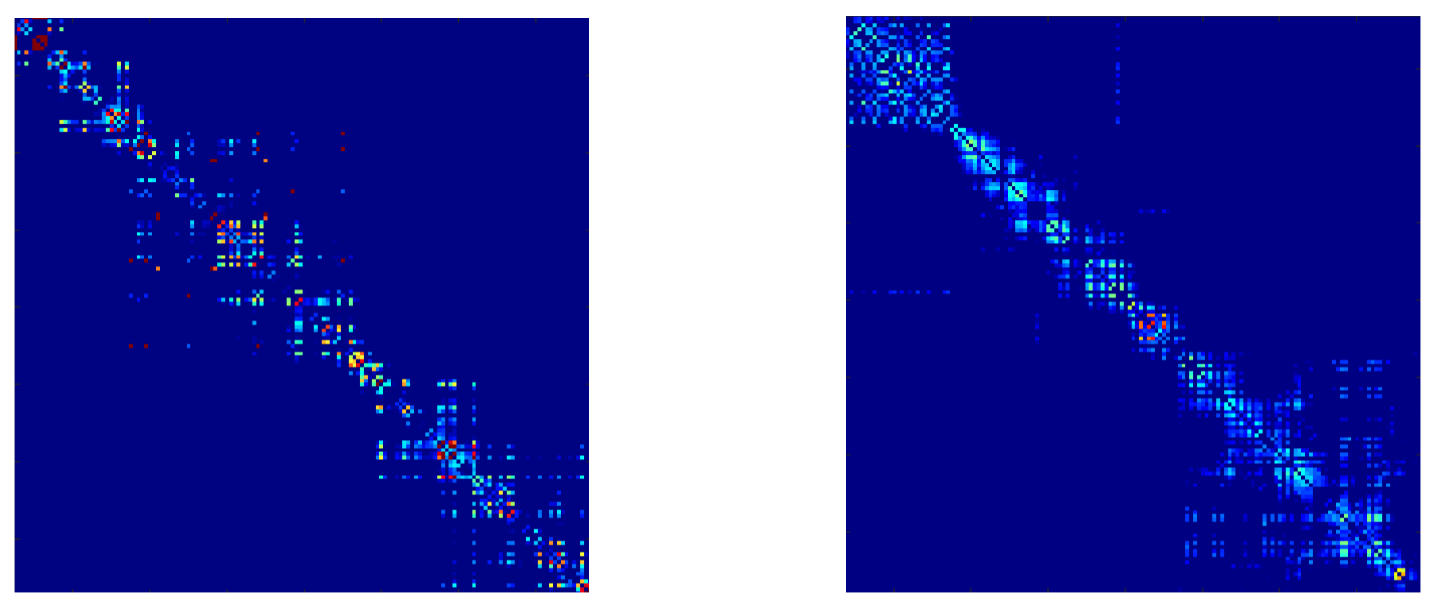
The similarity graph of the consensus graph learned by our method on the Caltech7 dataset under 30% and 50% missing-view rates are presented in Figure 2. As observed in the left sub-figure, the learned graph exhibits a clear block-diagonal structure, effectively capturing the underlying cluster structure. More importantly, even under a high missing rate of 50%, the consensus graph maintains a pronounced block-diagonal pattern, demonstrating the robustness and effectiveness of our approach in handling incomplete multi-view data.

Figure 2. The consensus graph learned by our method from the Caltech7 with 30% and 50% missing views.

Runtime and Complexity Analysis

To further evaluate the efficiency of the proposed TCGL method, we report both empirical runtime statistics and a theoretical analysis of computational complexity. Table 6 summarizes the total running time and the average per-iteration time on four benchmark datasets under a 30% missing rate.

• Empirical runtime analysis: As shown in Table 7, TCGL achieves competitive efficiency on small- and medium-scale datasets such as ORL, UCI, and Caltech101-7, with average iteration times all within a few seconds. On the larger Animal dataset, the computation becomes more demanding due to the tensor SVD step, which is theoretically the dominant cost of the algorithm. Nevertheless, TCGL remains practically executable and converges within a reasonable number of iterations (typically 20–30), making the overall runtime manageable even for larger data.
  Table 7. Runtime statistics of TCGL on four benchmark datasets.

  Dataset	Total Time (s)	Avg. Iter Time (s)
  Caltech101-7 (30% missing)	66.0997	3.1071
  UCI (30% missing)	52.6787	2.0615
  ORL (30% missing)	5.5199	0.2217
  Animal (30% missing)	1576.0215	131.3351

• Theoretical complexity analysis: According to the decomposition of Algorithm 1, the main computational costs arise from: (i) the update of S, requiring $O(n^{2}logn)$ due to row-wise simplex projection; (ii) the closed-form update of each $Z^{\left(v\right)}$, with complexity $O\left(n_v^2\right)$ per view; (iii) the computation of the c smallest eigenvectors for updating F, with cost $O\left(n^{2}c\right)$; and (iv) the tensor SVD for updating J, with complexity $O\left(V·(n_1{n}_{2}min(n_1,n_2))\right)$, which dominates the per-iteration computation. By aggregating these components, the overall per-iteration complexity of TCGL can be expressed as $O\left(V·(n_1{n}_{2}min(n_1,n_2))+n^{2}logn+n^{2}c\right)$.

Algorithm 1 Tensorized Consensus Graph Learning for Incomplete Multi-View Clustering with Confidence Integration

Require: Multi-view dataset $\mathbf{X}={\left\{{\mathbf{X}}^{\left(v\right)}\in {\mathbb{R}}^{d_v\times n}\right\}}_{v=1}^V$, trade-off parameters $\alpha ,\beta >0$, weight vector $\omega >0$ (initialized as ${\omega }_i=1/min(n_1,n_2)$ and kept fixed), and cluster number c. 1: Initialize $\mathcal{Q}=\mathcal{J}=\mathbf{0}$, and set $\rho$ ($\rho \in (1,2]$). 2: while${\displaystyle \frac{\parallel {\mathbf{F}}^{\left(k\right)}-{\mathbf{F}}^{(k-1)}{\parallel }_F}{\parallel {\mathbf{F}}^{(k-1)}{\parallel }_F}}>{10}^{-4}$  and  $k<30$  do 3:      for $\forall v=1,\dots ,V$ do 4:            Update ${\mathbf{S}}^{\left(v\right)}$ by solving the problem in Equation (26). 5:      end for 6:      for $\forall v=1,\dots ,V$ do 7:            Update ${\mathbf{Z}}^{\left(v\right)}$ by solving the problem in Equation (14). 8:      end for 9:       Update $\mathcal{J}$ by solving the problem in Equation (34). 10:     Update $\mathcal{Q}$ by $\mathcal{Q}=\mathcal{Q}+\rho (\mathcal{Z}-\mathcal{J})$. 11:     Update $\mathbf{F}$, which is formed by c eigenvectors of ${\mathbf{L}}_s={\mathbf{D}}_s-{\displaystyle \frac{{\mathbf{S}}^T+\mathbf{S}}{2}}$ corresponding to the c smallest eigenvalues. 12:     Update the weight ${\mathbf{\alpha }}_{\mathbf{v}}$ by solving the problem in Equation (11). 13:     Update $\mathbf{\rho }$ by $\mathbf{\rho }=\mathbf{\mu }\mathbf{\rho }$. 14: end while Ensure: The learned consensus graph $\mathbf{S}$ and the clustering labels obtained by performing k-means on the spectral embedding $\mathbf{F}$.

• Discussion: Although tensor operations contribute significantly to the computational cost, TCGL benefits from fast convergence and maintains competitive runtime compared with existing tensor-based multi-view clustering methods. The results demonstrate that TCGL achieves a favorable balance between clustering accuracy and computational efficiency.

5.3. Parameter Sensitivity Analysis

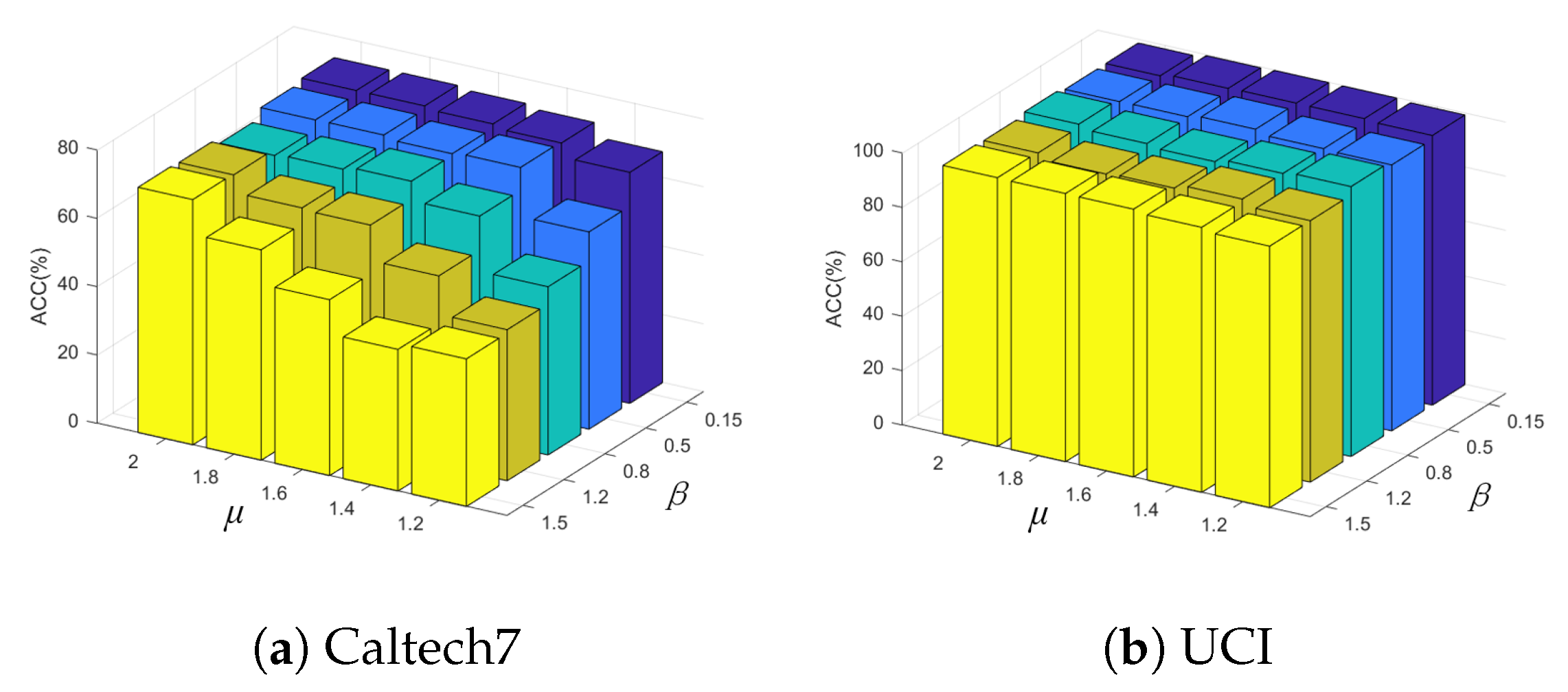
From the experimental results shown in Figure 3a, it can be observed that the proposed method is sensitive to the parameter $\mu$, where the best performance is achieved when $\mu =2$ and $\beta =0.15$. This indicates that selecting appropriate parameters for the tensor low-rank processing module is crucial, and it plays an important role in improving clustering performance. By combining the subfigures (a) and (b) in Figure 3, we can observe that the proposed TCGL model consistently demonstrates superior clustering results across different datasets.

Figure 3. Parameters analysis: The performances in terms of ACC when using different trade-off parameters $\mu$ and $\beta$ on the Caltech7 and UCI datasets, respectively.

5.4. Visualization

As shown in Figure 4, we visualize the t-SNE results on the Caltech7 and UCI datasets. These visualizations clearly demonstrate that TCGL effectively reveals an underlying clustering structure.

Figure 4. t-SNE visualization results at 30% incomplete rate, where the numbers represent different classes. (a–c) Original features, HCLS_CGL representations, and TCGL representations on the Caltech7 dataset. (d–f) Original features, HCLS_CGL representations, and TCGL representations on the UCI dataset.

5.5. Convergence Analysis

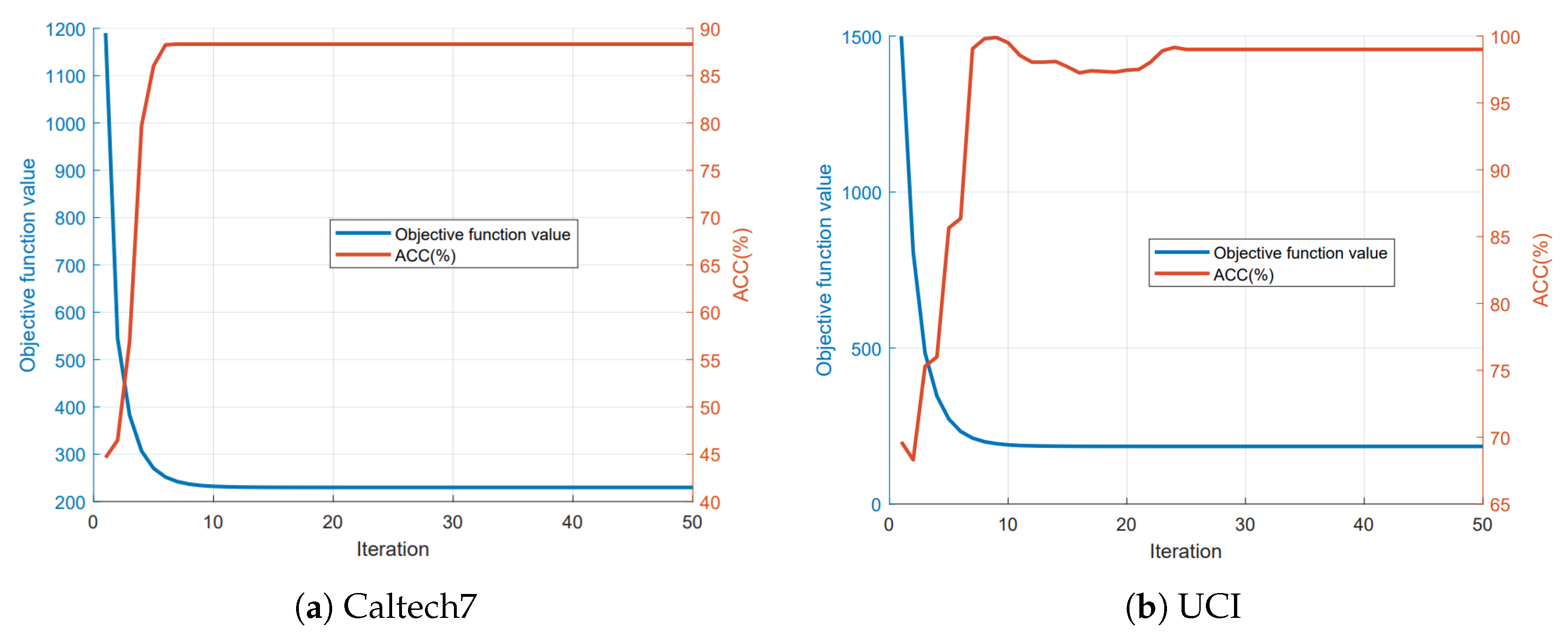
As previously mentioned, the complex objective function is decomposed into six convex subproblems. Minimizing each subproblem leads to a continuous decrease in the objective value. This implies that during the alternating update process of these variables, the loss of objective function (5) remains monotonically decreasing. In Figure 5, we present the variation of the objective function loss with the number of iterations on the Caltech7 and UCI datasets with a missing-view rate of 30%. From the figure, it can be observed that the objective loss consistently decreases and quickly converges to a stable state, which confirms the good convergence property of the proposed optimization algorithm.

Figure 5. The objective function value and clustering accuracy versus the number of iterations of the proposed method on the (a) Caltech7 dataset where the missing-view rate is set as 30% and the (b) UCI dataset where the missing-view rate is set as 10%.

6. Conclusions

In this paper, we propose a Tensorized Consensus Graph Learning with Confidence Integration (TCGL) method to address challenges in incomplete multi-view clustering, including inefficient local information utilization, noise sensitivity, and insufficient capture of higher-order cross-view correlations. By filtering missing samples to preserve valid data structure, employing tensor nuclear norm sparsification to model multi-view higher-order relationships, and integrating confidence-based probability matrices for noise robustness, TCGL enables effective clustering of incomplete multi-view data. Experimental evaluations across benchmark datasets demonstrate its superiority over state-of-the-art methods in capturing cross-view complementary information and handling data incompleteness. Notably, on the Caltech7 dataset with 30% missing rate, TCGL achieved the most significant improvements, outperforming the second-best method by 25.34% in ACC and 39.89% in NMI. Future research will explore optimizing TCGL for large-scale scenarios and integrating it with deep learning for complex non-linear data analysis.

Although TCGL achieves strong results, several directions remain open. The tensor and spectral operations may become computationally demanding on very large datasets, motivating more efficient large-scale approximations. The row-sum constraint on $Z^{\left(v\right)}$ may also be less suitable when data neighborhoods are highly irregular. Moreover, our experiments assume MCAR missingness, while behavior under MNAR settings requires further study. Extending TCGL toward neural clustering frameworks and learning adaptive view-specific weights are also promising directions for improving flexibility and modeling power.

References

1. Wang, H.; Chen, Y.; Yao, M.; Liu, W.; Peng, J.; Fu, X. Tensor Completion Framework by Graph Refinement for Incomplete Multi-view Clustering. IEEE Trans. Multimed. 2025, 1–14. [Google Scholar] [CrossRef]
2. Zhang, D.; Li, H.; He, D.; Liu, N.; Cheng, L.; Wang, J.; Han, J. Unsupervised Pre-training with Language-Vision Prompts for Low-Data Instance Segmentation. IEEE Trans. Pattern Anal. Mach. Intell. 2025, 47, 8642–8657. [Google Scholar] [CrossRef] [PubMed]
3. Peng, J.; Li, M.; Wang, B.; Wang, H. Omni contextual aggregation networks for high-fidelity image inpainting. IEEE Trans. Circuits Syst. Video Technol. 2025, 35, 6129–6144. [Google Scholar] [CrossRef]
4. Liu, Y.; Li, C.; Xu, S.; Han, J. Part-whole relational fusion towards multi-modal scene understanding. Int. J. Comput. Vis. 2025, 133, 4483–4503. [Google Scholar] [CrossRef]
5. Jiang, G.; Peng, J.; Wang, H.; Mi, Z.; Fu, X. Tensorial multi-view clustering via low-rank constrained high-order graph learning. IEEE Trans. Circuits Syst. Video Technol. 2022, 32, 5307–5318. [Google Scholar] [CrossRef]
6. Yao, M.; Wang, H.; Chen, Y.; Fu, X. Between/within view information completing for tensorial incomplete multi-view clustering. IEEE Trans. Multimed. 2024, 27, 1538–1550. [Google Scholar] [CrossRef]
7. Zhang, D.; Cheng, L.; Liu, Y.; Wang, X.; Han, J. Mamba capsule routing towards part-whole relational camouflaged object detection. Int. J. Comput. Vis. 2025, 133, 7201–7221. [Google Scholar] [CrossRef]
8. Liu, Y.; Cheng, D.; Zhang, D.; Xu, S.; Han, J. Capsule Networks With Residual Pose Routing. IEEE Trans. Neural Netw. Learn. Syst. 2024, 36, 2648–2661. [Google Scholar] [CrossRef]
9. Feng, L.; Wang, H.; Jin, B.; Li, H.; Xue, M.; Wang, L. Learning a Distance Metric by Balancing KL-Divergence for Imbalanced Datasets. IEEE Trans. Syst. Man Cybern. Syst. 2019, 49, 2384–2395. [Google Scholar] [CrossRef]
10. Wang, H.; Yao, M.; Jiang, G.; Mi, Z.; Fu, X. Graph-Collaborated Auto-Encoder Hashing for Multiview Binary Clustering. IEEE Trans. Neural Netw. Learn. Syst. 2024, 35, 10121–10133. [Google Scholar] [CrossRef]
11. Hu, Z.; Nie, F.; Chang, W.; Hao, S.; Wang, R.; Li, X. Multi-view spectral clustering via sparse graph learning. Neurocomputing 2020, 384, 1–10. [Google Scholar] [CrossRef]
12. Cai, B.; Wang, H.; Yao, M.; Fu, X. Focus more on what? Guiding multi-task training for end-to-end person search. IEEE Trans. Circuits Syst. Video Technol. 2025, 35, 7266–7278. [Google Scholar] [CrossRef]
13. Liu, X.; Li, M.; Tang, C.; Xia, J.; Xiong, J.; Liu, L.; Kloft, M.; Zhu, E. Efficient and effective regularized incomplete multi-view clustering. IEEE Trans. Pattern Anal. Mach. Intell. 2020, 43, 2634–2646. [Google Scholar] [CrossRef] [PubMed]
14. Wen, J.; Liu, C.; Xu, G.; Wu, Z.; Huang, C.; Fei, L.; Xu, Y. Highly confident local structure based consensus graph learning for incomplete multi-view clustering. In Proceedings of the IEEE/CVF Conference on Computer Vision and Pattern Recognition, Vancouver, BC, Canada, 17–24 June 2023; pp. 15712–15721. [Google Scholar]
15. Liu, J.; Wang, C.; Gao, J.; Han, J. Multi-view clustering via joint nonnegative matrix factorization. In Proceedings of the 2013 SIAM International Conference on Data Mining, SIAM, Austin, TX, USA, 2–4 May 2013; pp. 252–260. [Google Scholar]
16. Khan, M.A.; Khan, G.A.; Khan, J.; Khan, M.R.; Atoum, I.; Ahmad, N.; Shahid, M.; Ishrat, M.; Alghamdi, A.A. Multi-view clustering based on multiple manifold regularized non-negative sparse matrix factorization. IEEE Access 2022, 10, 113249–113259. [Google Scholar] [CrossRef]
17. Luong, K.; Nayak, R.; Balasubramaniam, T.; Bashar, M.A. Multi-layer manifold learning for deep non-negative matrix factorization-based multi-view clustering. Pattern Recognit. 2022, 131, 108815. [Google Scholar] [CrossRef]
18. Kumar, S.; Ying, J.; Cardoso, J.V.d.M.; Palomar, D.P. A unified framework for structured graph learning via spectral constraints. J. Mach. Learn. Res. 2020, 21, 1–60. [Google Scholar]
19. Wang, H.; Yao, M.; Chen, Y.; Xu, Y.; Liu, H.; Jia, W.; Fu, X.; Wang, Y. Manifold-based incomplete multi-view clustering via bi-consistency guidance. IEEE Trans. Multimed. 2024, 26, 10001–10014. [Google Scholar] [CrossRef]
20. Chen, M.S.; Wang, C.D.; Lai, J.H. Low-rank tensor based proximity learning for multi-view clustering. IEEE Trans. Knowl. Data Eng. 2022, 35, 5076–5090. [Google Scholar] [CrossRef]
21. Wang, H.; Jiang, G.; Peng, J.; Deng, R.; Fu, X. Towards adaptive consensus graph: Multi-view clustering via graph collaboration. IEEE Trans. Multimed. 2022, 25, 6629–6641. [Google Scholar] [CrossRef]
22. Kilmer, M.E.; Braman, K.; Hao, N.; Hoover, R.C. Third-order tensors as operators on matrices: A theoretical and computational framework with applications in imaging. SIAM J. Matrix Anal. Appl. 2013, 34, 148–172. [Google Scholar] [CrossRef]
23. Kilmer, M.E.; Martin, C.D. Factorization strategies for third-order tensors. Linear Algebra Its Appl. 2011, 435, 641–658. [Google Scholar] [CrossRef]
24. Zhang, Z.; Ely, G.; Aeron, S.; Hao, N.; Kilmer, M. Novel methods for multilinear data completion and de-noising based on tensor-SVD. In Proceedings of the IEEE Conference on Computer Vision and Pattern Recognition, Columbus, OH, USA, 23–28 June 2014; pp. 3842–3849. [Google Scholar]
25. Wen, J.; Zhang, Z.; Xu, Y.; Zhang, B.; Fei, L.; Liu, H. Unified embedding alignment with missing views inferring for incomplete multi-view clustering. AAAI Conf. Artif. Intell. 2019, 33, 5393–5400. [Google Scholar] [CrossRef]
26. Ng, A.; Jordan, M.; Weiss, Y. On spectral clustering: Analysis and an algorithm. Adv. Neural Inf. Process. Syst. 2001, 14, 1–8. [Google Scholar]
27. Von Luxburg, U. A tutorial on spectral clustering. Stat. Comput. 2007, 17, 395–416. [Google Scholar] [CrossRef]
28. Feng, J.; Lin, Z.; Xu, H.; Yan, S. Robust subspace segmentation with block-diagonal prior. In Proceedings of the IEEE Conference on Computer Vision and Pattern Recognition, Columbus, OH, USA, 23–28 June 2014; pp. 3818–3825. [Google Scholar]
29. Kang, Z.; Peng, C.; Cheng, Q. Clustering with adaptive manifold structure learning. In Proceedings of the 2017 IEEE 33rd International Conference on Data Engineering (ICDE), Diego, CA, USA, 19–22 April 2017; pp. 79–82. [Google Scholar]
30. Liu, G.; Lin, Z.; Yan, S.; Sun, J.; Yu, Y.; Ma, Y. Robust recovery of subspace structures by low-rank representation. IEEE Trans. Pattern Anal. Mach. Intell. 2012, 35, 171–184. [Google Scholar] [CrossRef]
31. Nie, F.; Wang, X.; Jordan, M.; Huang, H. The constrained laplacian rank algorithm for graph-based clustering. AAAI Conf. Artif. Intell. 2016, 30, 1969–1976. [Google Scholar] [CrossRef]
32. Nie, F.; Li, J.; Li, X. Self-weighted multiview clustering with multiple graphs. In Proceedings of the IJCAI, Melbourne, Australia, 19–25 August 2017; pp. 2564–2570. [Google Scholar]
33. Zhan, K.; Zhang, C.; Guan, J.; Wang, J. Graph learning for multiview clustering. IEEE Trans. Cybern. 2017, 48, 2887–2895. [Google Scholar] [CrossRef] [PubMed]
34. Wu, J.; Xie, X.; Nie, L.; Lin, Z.; Zha, H. Unified graph and low-rank tensor learning for multi-view clustering. AAAI Conf. Artif. Intell. 2020, 34, 6388–6395. [Google Scholar] [CrossRef]
35. Wang, H.; Yang, Y.; Liu, B. GMC: Graph-based multi-view clustering. IEEE Trans. Knowl. Data Eng. 2019, 32, 1116–1129. [Google Scholar] [CrossRef]
36. Duchi, J.; Shalev-Shwartz, S.; Singer, Y.; Chandra, T. Efficient projections onto the l 1-ball for learning in high dimensions. In Proceedings of the 25th International Conference on Machine Learning, Helsinki, Finland, 5–9 July 2008; pp. 272–279. [Google Scholar]
37. Zhao, H.; Liu, H.; Fu, Y. Incomplete multi-modal visual data grouping. In Proceedings of the IJCAI, New York, NY, USA, 9–15 July 2016; pp. 2392–2398. [Google Scholar]
38. Shao, W.; He, L.; Yu, P.S. Multiple incomplete views clustering via weighted nonnegative matrix factorization with regularization. In Proceedings of the Joint European Conference on Machine Learning and Knowledge Discovery in Databases, Porto, Portugal, 7–11 September 2015; pp. 318–334. [Google Scholar]
39. Hu, M.; Chen, S. Doubly aligned incomplete multi-view clustering. arXiv 2019, arXiv:1903.02785. [Google Scholar] [CrossRef]
40. Shao, W.; He, L.; Lu, C.T.; Yu, P.S. Online multi-view clustering with incomplete views. In Proceedings of the 2016 IEEE International Conference on Big Data (Big Data), Washington, DC, USA, 5–8 December 2016; pp. 1012–1017. [Google Scholar]
41. Hu, M.; Chen, S. One-pass incomplete multi-view clustering. AAAI Conf. Artif. Intell. 2019, 33, 3838–3845. [Google Scholar] [CrossRef]
42. Liu, X.; Zhu, X.; Li, M.; Wang, L.; Zhu, E.; Liu, T.; Kloft, M.; Shen, D.; Yin, J.; Gao, W. Multiple kernel k k-means with incomplete kernels. IEEE Trans. Pattern Anal. Mach. Intell. 2019, 42, 1191–1204. [Google Scholar] [CrossRef] [PubMed]
43. Wang, H.; Zong, L.; Liu, B.; Yang, Y.; Zhou, W. Spectral perturbation meets incomplete multi-view data. arXiv 2019, arXiv:1906.00098. [Google Scholar] [CrossRef]
44. Wen, J.; Yan, K.; Zhang, Z.; Xu, Y.; Wang, J.; Fei, L.; Zhang, B. Adaptive graph completion based incomplete multi-view clustering. IEEE Trans. Multimed. 2020, 23, 2493–2504. [Google Scholar] [CrossRef]
45. Li, Z.; Tang, C.; Liu, X.; Zheng, X.; Zhang, W.; Zhu, E. Tensor-based multi-view block-diagonal structure diffusion for clustering incomplete multi-view data. In Proceedings of the 2021 IEEE International Conference on Multimedia and Expo (ICME), Shenzhen, China, 5–9 July 2021; pp. 1–6. [Google Scholar]
46. Xu, J.; Li, C.; Ren, Y.; Peng, L.; Mo, Y.; Shi, X.; Zhu, X. Deep Incomplete Multi-View Clustering via Mining Cluster Complementarity. In Proceedings of the AAAI Conference on Artificial Intelligence (AAAI), Online, 22 February–1 March 2022; pp. 8761–8769. [Google Scholar]
47. Wang, S.; Liu, X.; Liu, L.; Tu, W.; Zhu, X.; Liu, J.; Zhou, S.; Zhu, E. Highly-efficient incomplete large-scale multi-view clustering with consensus bipartite graph. In Proceedings of the IEEE/CVF Conference on Computer Vision and Pattern Recognition, New Orleans, LA, USA, 21–24 June 2022; pp. 9776–9785. [Google Scholar]
48. Liu, C.; Wu, Z.; Wen, J.; Xu, Y.; Huang, C. Localized sparse incomplete multi-view clustering. IEEE Trans. Multimed. 2022, 25, 5539–5551. [Google Scholar] [CrossRef]
49. Xia, W.; Gao, Q.; Wang, Q.; Gao, X. Tensor Completion-Based Incomplete Multiview Clustering. IEEE Trans. Cybern. 2022, 52, 13635–13644. [Google Scholar] [CrossRef] [PubMed]
50. Zhang, C.; Li, H.; Lv, W.; Huang, Z.; Gao, Y.; Chen, C. Enhanced tensor low-rank and sparse representation recovery for incomplete multi-view clustering. AAAI Conf. Artif. Intell. 2023, 37, 11174–11182. [Google Scholar] [CrossRef]
51. Wang, J.; Zhao, Z.; Dobigeon, N.; Chen, J. Joint Tensor and Inter-View Low-Rank Recovery for Incomplete Multiview Clustering. arXiv 2025, arXiv:2503.02449. [Google Scholar]
52. Wen, J.; Zhang, Z.; Zhang, Z.; Zhu, L.; Fei, L.; Zhang, B.; Xu, Y. Unified tensor framework for incomplete multi-view clustering and missing-view inferring. AAAI Conf. Artif. Intell. 2021, 35, 10273–10281. [Google Scholar] [CrossRef]
Disclaimer/Publisher’s Note: The statements, opinions and data contained in all publications are solely those of the individual author(s) and contributor(s) and not of MDPI and/or the editor(s). MDPI and/or the editor(s) disclaim responsibility for any injury to people or property resulting from any ideas, methods, instructions or products referred to in the content.
Article Metrics
Citations
Article Access Statistics
Multiple requests from the same IP address are counted as one view.