Monitoring and Prediction of Deformation and Failure of Roadway Surrounding Rock Based on Binocular Vision and Random Forest

Abstract

The deformation and failure of surrounding rock in underground roadways are governed by complex mechanical interactions and environmental factors, yet the fundamental scientific patterns behind these processes remain unclear. This lack of real-time, data-driven understanding limits the development of intelligent monitoring and prediction systems in mining engineering. To address this challenge, this study aims to establish an intelligent system for the dynamic monitoring and prediction of roadway surrounding rock deformation based on binocular vision and machine learning. An improved Semi-Global Block Matching (SGBM) algorithm is developed for real-time 3D deformation measurement, while a physical similarity model is constructed to visualize the deformation–failure evolution. The Random Forest (RF) algorithm is employed for deep deformation prediction, and its optimal parameters are determined by minimizing the mean square error. Experimental results show that the average measurement errors of the binocular vision method are 1.22 mm and 0.92 mm, outperforming total station monitoring. The gradient-enhanced Random Forest (GERF) model achieves RMSE values of 0.0164 and 0.0113, with R² values of 0.8856 and 0.8356, respectively. Compared with AdaBoost, XGBoost, and Vision Transformer models, GERF improves predictive accuracy by 7.82%, 8.68%, and 3.87%, respectively. These findings demonstrate the scientific feasibility and technical advantage of the proposed intelligent system, offering a new approach to understanding and predicting roadway deformation and failure in intelligent mining.

1. Introduction

With the increasing depth of coal mining, severe deformation and damage to roadways are becoming more frequent, leading to frequent safety accidents such as roadway collapse, roof fall, and sidewall spalling [1,2,3]. The stability of the surrounding rock in roadways is crucial not only for personnel safety but also for maintaining production efficiency. In deep mining environments, stress-induced deformation is dynamic and complex, further increasing the difficulty of monitoring and control. Therefore, accurate and continuous monitoring and effective prediction of surrounding rock deformation has become the core of smart mining research [4,5]. Against this backdrop, there is an urgent need for more adaptive, real-time, and accurate methods to monitor and predict the deformation and damage of the rock mass surrounding roadways, especially in dynamic and complex mining environments.

Traditional methods for monitoring surrounding rock deformation and damage, such as laser scanning, ground-penetrating radar, and conventional measuring instruments, often face numerous challenges, including high costs, complex operation, and difficulty in handling large datasets [6,7,8]. While these methods have value, they are insufficient in complex and variable mining environments, especially when real-time data acquisition is required [9,10,11]. For example, laser scanning is very effective in static environments, but it has limitations in underground mining operations because the underground working environment is often undesirable, such as insufficient lighting, dust, and the movement of machinery, all of which affect the accuracy and real-time performance of the system [11,12,13]. Photogrammetry, while useful, also has similar adaptability problems in environments with uniform texture, leading to difficulties in feature recognition and stereo matching [14,15,16]. Zhu, D. [17] analyzed the deformation mechanism of deep soft rock roadways through on-site investigation, mechanical modeling and numerical simulation. And developed a combined control technology of “roof corner anchor cable + rib anchor cable + concrete inverted arch + floor anchor cable” was proposed as a combined support technology, which has been successfully applied and monitored in roadway III4104 and confirmed. By analyzing the spatial distribution and rotation of the principal stress axis under three-dimensional stress conditions, Zuo, J. [18] studied the complex failure mechanism of roads, established mechanical and numerical models, and revealed how stress adjustment leads to failure. The research results were verified through on-site observations. Liu, G. [19] combined indoor experiments with three-dimensional discontinuous deformation analysis (3D DDA) and utilized a customized high-speed binocular vision experimental system to explore the movement characteristics of falling rocks. By analyzing the influences of the shape of the falling rocks, the height of the fall, the slope Angle and the release method, it is determined that the slope Angle and the height of the fall are the main factors affecting the speed of the falling rocks. The experimental results are highly consistent with the simulation results, verifying the accuracy of this method. Despite challenges such as poor lighting and adverse mining conditions, these remote sensing techniques provide a valuable complement to traditional point measurement methods by delivering comprehensive time-lapse data for better understanding of surrounding rock deformation and failure. However, laser scanning still has limitations, particularly in its application within complex environments and in terms of real-time performance.

Since the beginning of the 21st century, computer vision technology has gradually become an important tool for surrounding rock monitoring and prediction. Du, Y.X. [20] investigated the key technologies of visual inspection systems and their applications in tunneling sites and predicted the critical technologies that need to be developed in the future. Han, Z. [21] established a full-plane strain model of a rectangular roadway considering the deflection of the principal stress axis, derived analytical solutions for the stress and plastic zone distributions, and analyzed the effect of stress space rotation on roadway stability. The results show that stress deflection leads to asymmetric failure and rapid expansion. Shen, Y. [22] studied the asymmetric deformation and failure of fully mechanized collapse roadways in close-range thick coal seams through numerical simulation and field tests and proposed an asymmetric support optimization scheme. The results show that the non-uniform stress generated by the residual coal pillar can lead to butterfly failure, while the proposed asymmetric support scheme can effectively maintain the stability of the roadway. Chai, J. [23] established a force and deformation model based on optical fiber sensing for monitoring the loose areas of the roadway floor. He introduced a compression coefficient (ξ) to quantify rock compression and demonstrated that distributed optical fiber technology can effectively track the development, displacement and stress of the loose areas in real time during mining operations. Liang, MF [24] developed a cubic three-dimensional stress sensor based on fiber Bragg grating technology. Experiments demonstrated that the sensor achieves a triaxial sensitivity of 25.51–24.86 pm/MPa within the 0–50 MPa range, with a measurement error below 4%. The sensor exhibits good linearity and repeatability, providing a high-precision tool for safety monitoring in underground engineering such as coal mines and tunnels. Zhang, T. [25] conducted large-scale physical model tests to explore the dynamic instability of the surrounding rock of deeply buried roadways under plateau stress and dynamic disturbances. The results show that the increase in disturbance intensity and the change in disturbance position significantly affect crack propagation and failure, and stress concentration occurs at the arch shoulder and point b. Cheng, J. [26] addressed the issue of insufficient binocular vision positioning accuracy in coal mining roadheaders by establishing a spatial circular feature projection error model and a structural parameter analysis model. The study systematically analyzed the effects of imaging errors and sensor parameters on measurement accuracy. Experimental results validated the reliability and precision of the pose measurement system, providing technical support for improving the efficiency of intelligent coal mining operations. Mahdevari S. [27,28] proposed a Particle Swarm Optimization-based Adaptive Neuro-Fuzzy Inference System (PSO-ANFIS) model to predict the maximum roof displacement in the roadways of the Tabas coal mine. The results demonstrated that this model outperformed other methods in terms of accuracy and generalization ability, aiding in the identification of unstable zones and the formulation of support strategies. Additionally, the developed Improved Support Vector Regression (ISVR) model accurately predicted the stability of tailgate roadways in mechanized longwall mining, showing a high agreement with measured data (R² = 0.91) and outperforming Artificial Neural Networks and multivariate linear regression models.

In summary, the application of binocular vision methods in roadway deformation and failure monitoring is relatively mature; however, most existing studies are based on experiments simulating static roadway environments under idealized conditions [29,30,31]. Meanwhile, traditional stereo matching techniques face challenges when dealing with homogeneous surface textures commonly found in underground roadways. In the field of roadway deformation prediction, current research mainly focuses on predicting the deformation amount at the same location in the surrounding rock [32,33]. To address these issues, the general methodological framework of this study is structured into three main components: (1) experimental modeling of roadway deformation and failure using a physical similarity model; (2) binocular vision–based monitoring and data acquisition with an improved stereo matching algorithm; and (3) deformation prediction through the Gradient-Enhanced Random Forest (GERF) model trained on the visual monitoring data. This integrated framework enables a closed-loop process from deformation observation to model-based prediction and validation [34]. Although the proposed method aims to improve the accuracy of deformation monitoring and prediction, the fundamental research problem addressed in this study is to reveal the intrinsic coupling mechanism between the deformation-failure evolution of roadway surrounding rock under complex dynamic stress conditions and its visual characteristics [35,36]. Understanding this coupling mechanism provides a theoretical foundation for developing intelligent, data-driven roadway monitoring and prediction systems.

2. Principle

2.1. Monitoring Principles

2.1.1. Binocular Vision Algorithm

The binocular vision approach operates on the concept of disparity. It employs a pair of cameras, spaced at a specific interval, to record the same subject simultaneously. The discrepancy in the position of the pixels representing the object in the left and right images is referred to as disparity [37]. By determining the disparity of matching points across the images, and applying the principle of triangulation, the 3D information of the object can be obtained [38].

As shown in Figure 1, the parallel binocular vision model represents the ideal configuration. The experiment was conducted under low-light conditions (100 lux) to closely simulate the dim environment typically found underground. When capturing images at close range, the binocular vision system can achieve higher depth resolution; however, it may be constrained by a limited field of view, resulting in certain areas not being captured. When capturing images at a greater distance, the field of view becomes wider; however, the accuracy of the depth information may decrease. Therefore, a distance of 10 m between the binocular camera and the monitoring point was selected. During image acquisition, occlusions and reflections were minimized to avoid interference with the field of view and the acquisition of depth information. The detailed camera parameters are provided in Table 1.

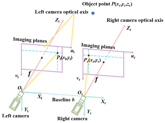
Figure 1. Principle of parallel binocular vision monitoring.

Table 1. Parameter Table of Binocular Cameras.

Camera Parameters	Configuration
Lens focal length	3.4 mm
Lens perspective	H 71°, V 55°
Image sensor	AR0135
Single pixel size	3.75 μm × 3.75 μm
Binocular baseline	60 mm
Image resolution	1280 × 720
Video capture frame rate	2560 × 720@30FPS
Communication interface	USB3.0, UVC protocol, driver-free
Measurement range	0.3 m~3.5 m

The baseline distance is denoted as b, and the monitoring point P(x_c,y_c,z_c) of the roadway surrounding rock is cast onto the optical centers of the left and right cameras O_l and O_r. The projections on the left and right image planes are denoted as P_l(x_l,y_l) and P_r(x_r,y_r) [39]. The difference between the projected points P_l and P_r is the difference in their x-axis coordinates, as shown in Formula (1).

$$disparity=x_l-x_r$$

(1)

where the unit of measurement for disparity is in pixels.

By utilizing the parallax measurement and the principle of the similar triangles theorem, the three-dimensional coordinates of point P relative to the optical center of the left camera can be determined:

$$\left\{\begin{array}{l}{x}_c={\displaystyle \frac{b{x}_l}{disparity}}\\ y_c={\displaystyle \frac{b{y}_l}{disparity}}\\ z_c={\displaystyle \frac{bf}{disparity}}\end{array}\right.$$

(2)

f represents the focal length of the camera, which is the measurement from the central point of the camera to the plane where the projection occurs; B denotes the baseline, which is the separation distance between the left eye, O_l, and the right eye, Or.

2.1.2. Improved SGBM Algorithm

The central step of binocular stereo vision is stereo matching, which calculates parallax by identifying matching pixels with similar characteristics on the two images [40]. The SGBM algorithm is a stereo-matching method provided in Opencv 4.11.0. In its cost calculation step, the SAD_BT cost is calculated by cost fusion, which provides the basis for subsequent cost aggregation [41]. The SAD_BT cost of a point P is the sum of all BT costs in the surrounding neighborhood, the formula for the calculation is given below. Where Np is the size of the neighborhood.

$$B{T}_{SAD}(p,d)={\displaystyle \sum _{q\in N_p}B}T(q,d)$$

(3)

where BT(q, d) is the BT cost function; q is a pixel in the neighborhood; d is parallax.

In this algorithm, the BlockSize parameter represents the neighborhood size in the above formula, which affects the accuracy of the disparity map calculation. In real-world usage, the choice of BlockSize should be determined by the image’s texture complexity. as it defines the size of the matching block used in the cost calculation. To observe the impact of the BlockSize parameter on the disparity map results, the SGBM (Semi-Global Block Matching) algorithm is utilized for calculating the disparity map. Disparity results are obtained by selecting different sizes for the BlockSize parameter. Figure 2a shows the disparity test image selected from Middlebury. The objects in the image have a strong layering effect, and the texture is diverse, which allows for the evaluation of the image matching performance.

Figure 2. Stereo matching results of different BlockSizes: (a) Original images; (b) BlockSize = 5; (c) BlockSize = 7; (d) BlockSize = 9.

Furthermore, based on the above experimental analysis, the role of the BlockSize parameter can be summarized as follows: when BlockSize is small, disparity estimation is performed over a smaller range, capturing finer details but resulting in increased noise and poorer overall disparity map quality [42]. As BlockSize increases, the disparity estimation becomes more global, producing smoother disparity maps with clearer edges and improved overall performance. However, when BlockSize becomes excessively large (BlockSize = 9), the disparity map becomes overly smooth with very few noise points, but this results in the loss of many details. Additionally, using a fixed BlockSize increases the complexity of adjusting other parameters.

When computing the disparity map using the SGBM algorithm, the BlockSize parameter is fixed, meaning that a uniform block size is used across the entire image to calculate the SAD_BT cost. A fixed BlockSize may not adapt well to the varying characteristics of different scenes and images. For images with diverse textures, structures, and noise levels, employing a fixed BlockSize can lead to a decline in the quality of the disparity map. This paper presents an adaptive BlockSize SGBM algorithm incorporating multi-scale processing to mitigate the challenge. The main objectives of multi-scale processing are as follows: to adapt to objects of different scales, to handle regions with varying texture levels, and to enhance the robustness of the algorithm. As shown in Figure 3, the image pyramid, by constructing a set of images at different resolutions, allows for the search of objects at various scales. Multi-scale processing is achieved through image pyramid operations, which improve matching accuracy and robustness in scenes with varying depth changes.

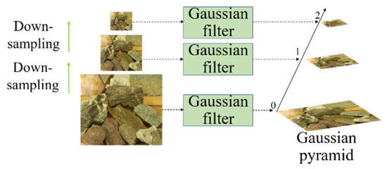
Figure 3. Principle of Gaussian image pyramid.

The SGBM algorithm uses a fixed window size to calculate disparity. However, in real images, the depth variation may differ across different regions, so using a fixed window size cannot effectively adapt to these variations. The adaptive window size method allows for the use of different window sizes in different regions, enabling more accurate capture of depth changes. This method fine-tunes the balance between computational efficiency and the accuracy of the disparity map. For example, in texture-rich regions, a larger window is used to achieve better local matching performance.

The main improvement of this algorithm lies in the determination of the matching BlockSize, and thus, this section focuses on explaining the algorithm improvements in this area. First, a fixed-size image block is selected. Then, the image gradient and contrast within the block area are calculated. Based on the computed image gradient and contrast, the BlockSize is recalculated. Finally, the new BlockSize is used to compute the block matching cost.

The image gradient is calculated using the Sobel differential operator, which can extract edge information from the image and assess the richness of its texture. The contrast of the gradient image is then computed, and based on the contrast information, the BlockSize is recalculated, as shown in the following Formula (4).

$$block\_size=\max (a,\min ({\displaystyle \frac{c}{ct}},b))$$

(4)

where BlockSize is the calculated BlockSize; c is the calculated contrast; ct is a predefined contrast threshold; b is the highest value for the set BlockSize; a is the minimum value of the set BlockSize.

Given the multi-scale processing method and the adaptive BlockSize method mentioned above, these two methods are combined to perform stereo matching on the binocular images. Figure 4 shows the overall algorithm flowchart after integrating the two improved algorithms.

Figure 4. The improved stereo matching algorithm steps.

2.2. Prediction Principle

The process of roadway deformation and failure is intricate and affected by a multitude of elements, including geological formations, characteristics of the rock, among others. Hence, predicting the deep deformation of the surrounding rock accurately solely by examining the deformation of the roof is challenging [43]. Nonetheless, roof deformation serves as an indication of the transmission of deformation from the deeper surrounding rock, and there exists a certain nonlinear relationship between them. Monitoring roof deformation can provide a general approximation of the deformation in the deeper surrounding rock, which in turn enables the forecasting of the deformation trend within the deeper surrounding rock [44].

RF is used to establish a forecasting model between roadway roof deformation and deep surrounding rock deformation and failure. The core of RF algorithm lies in the construction of decision trees. By integrating several decision trees, it enhances the overall model’s generalization ability. In regression problems, the strategy of Random Forest is to integrate the output values of each tree, and the ultimate prediction is determined by averaging or via a voting process [45]. RF regression method can effectively handle high-dimensional feature data and offers high prediction accuracy [46]. It performs well in regression problems, as shown in Formula (5).

$${\widehat{\mathrm{y}}}_{rf}={\displaystyle \frac{1}{N}}{\displaystyle {\sum }_{i=1}^N{\widehat{y}}_i}$$

(5)

Assuming there are n trees, and the prediction output of each tree is ${\widehat{y}}_i$, the final prediction output of RF is the average of these individual predictions.

The Random Forest regression method is effective in handling high-dimensional feature data and possesses high prediction accuracy. While Random Forest is built using a collection of decision trees, it may suffer from overfitting when the dataset contains a large amount of noise or outliers. Additionally, Random Forest has relatively poor handling capacity when dealing with datasets that have fewer features. To address this issue, in this study, a gradient boosting regression approach is employed to improve the Random Forest algorithm through ensemble learning, aiming to enhance overall performance by combining multiple models. Gradient boosting refers to an iterative process in which new decision trees are trained to fit the residuals of the initial model. These trees are then sequentially added to the ensemble, gradually reducing the overall residual error of the model. The specific implementation process is as follows: first, a gradient boosting regression model is trained using the dataset, and the residuals of this model are computed. Then, the original data along with the residuals are used to train a Random Forest regression model. Finally, the gradient boosting regression model and the Random Forest regression model are integrated to form a Gradient-Enhanced Random Forest [47]. This integrated model is then used for ensemble prediction to obtain the final results. This improved version of the Random Forest model is renamed as the Gradient-Enhanced Random Forest (GERF). Figure 5 shows the logical flowchart for model development and validation

Figure 5. Ensemble Prediction Process of the Gradient-Enhanced Random Forest (GERF).

3. Monitoring Experiment

3.1. Monitoring Experiment Design

This paper is based on the actual rock layer distribution of a coal mine working face and constructs a physical similarity model [48]. The prototype of the roadway is a rectangular roadway with a burial depth of approximately 370 m, an average coal seam thickness of 5.09 m. And roadway cross-sectional dimensions of approximately 5.3 m × 3.8 m (width × height). The geometric similarity ratio is 1:30. The experiment uses a model built on a platform with dimensions of 1.2 m × 1.2 m × 0.12 m (width × height × thickness). The coal seam thickness is 15 cm, the overlying rock thickness is 55 cm, and the roadway size is 18 cm × 13 cm × 12 cm (width × height × thickness). The experiment uses a hydraulic jack to incrementally load the model from the top, simulating the rock layer load on the roof.

As shown in Figure 6, the setup includes hydraulic jacks applying load to simulate roof pressure, and a dial gauge measuring roadway deformation and failure. A binocular camera captured images every 2 s (2560 × 720 resolution), with a computer handling control and storage. The NTS-332R10M total station recorded marker point coordinates for comparison with binocular vision results. Due to the model’s uniform surface, artificial markers were added for accurate deformation tracking.

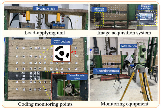
Figure 6. Monitoring equipment layout diagram.

The accuracy of binocular vision primarily depends on hardware configuration and environmental adaptability. Factors such as camera resolution, baseline distance, and calibration errors directly affect the precision of depth estimation. Additionally, variations in lighting, low-texture surfaces, or dynamic occlusions can lead to failures in stereo matching. At the algorithmic level, the choice of stereo matching methods like local matching or global optimization involves a trade-off between real-time performance and noise robustness. Post-processing strategies, such as filtering or interpolation, influence the smoothness of the final output and the preservation of fine details. Moreover, computational resource limitations constrain the real-time application of complex algorithms like Semi-Global Matching (SGM), necessitating a balance between performance and efficiency through hardware acceleration or algorithm simplification.

3.2. Stereo Camera Calibration

The camera calibration experiment uses the Zhang Zhengyou Calibration Method for calibration. As shown in Figure 7, a chessboard pattern with a size of 12 × 8 is used for calibrating the camera. According to the principles of Zhang Zhengyou’s calibration method, the checkerboard pattern is placed in different poses, and 12 sets of images are captured for calibration. Finally, the calibration is performed using the stereo vision calibration tool in MATLAB R2024b (24.2.0.2712019) [49].

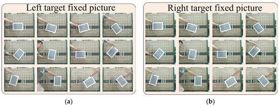
Figure 7. Camera calibration image: (a) Left eye camera; (b) Right eye camera.

Figure 8 illustrates that the calibration board images were taken using the stereo camera setup. The calibration board was placed in different poses in front of the model, with a distance approximately equal to that of the cameras. A total of 12 sets of images were taken for stereo calibration.

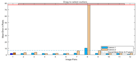
Figure 8. Initial reprojection error.

The reprojection error during the calibration process was analyzed, as shown in Figure 8. The chessboard was placed and photographed in 12 different poses. Based on the captured images, the reprojection errors were calculated. Among the 12 datasets, only the eighth set exhibited a significantly larger error. This was due to severe distortion of the chessboard during the capture of the eighth set. However, since the remaining data were sufficient for calibration, the eighth set was directly excluded.

After removing the images with large errors, the calibration is recalculated, and the results are shown in Figure 9. The blue bar chart represents the reprojection error for the left camera’s calibration results, while the orange bar chart represents the reprojection error for the right camera’s calibration results. As shown in the figure, the reprojection error for the left camera is generally larger, with the maximum reprojection error being 0.24 pixels. Reprojection error refers to the difference between the actually observed image points and the points projected onto the image plane through 3D reconstruction. It is an important indicator for measuring the system calibration accuracy and 3D reconstruction accuracy. For applications requiring millimeter-level precision, such as deformation monitoring of underground mine roadways, a reprojection error of less than one pixel is generally considered acceptable. The average reprojection error for both cameras is 0.17 pixels, which meets the requirements for stereo vision 3D reconstruction.

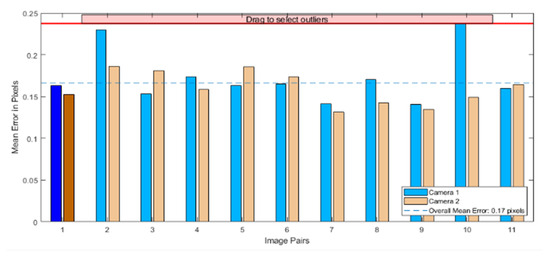
Figure 9. Optimization of reprojection error.

Figure 10 shows the reconstructed 3D spatial relationship from calibration between the board and cameras. The calibration board is positioned in various orientations, and it is essentially in the same plane, with a distance of approximately 1 m from the cameras, which is consistent with the actual distance.

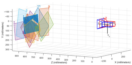
Figure 10. The pose relationship between the camera and the calibration plate.

The calibration results for the two cameras are shown in Table 2. From the calibration results, it can be observed that the parameters of the two cameras are quite similar, which is due to the fact that both cameras use lenses of the same model. In addition, the horizontal translation value between the two cameras is 60.9967 mm, which is consistent with the baseline distance between the stereo cameras, further verifying the accuracy of the calibration results.

Table 2. Camera calibration results.

Camera Parameters	Left Eye Camera	Right-Eye Camera
Intrinsic matrix	$\left[\begin{array}{ccc}546.5454& 0& 604.6869\\ 0& 546.7929& 341.1595\\ 0& 0& 1\end{array}\right]$	$\left[\begin{array}{ccc}544.0559& 0& 611.6199\\ 0& 544.6292& 336.0049\\ 0& 0& 1\end{array}\right]$
Radial distortion	(0.0126, −0.2808, 0.6969)	(−0.0029, −0.1095, 0.0327)
Tangential distortion	(9.4031 × 10−4, −0.0035)	(0.0016, −7.0767 × 10−4)
Translation vector	(−60.9967, −0.8824, −6.2671)
Rotation matrix	$\left[\begin{array}{ccc}0.9999& 0.0003& -0.0103\\ -0.0004& 1.0& -0.0041\\ 0.0103& 0.0041& 0.9999\end{array}\right]$

3.3. Stereo Image Processing

3.3.1. Feature Point Recognition

In the experiment, encoded reference points were arranged on the model to monitor the deformation of the surrounding rock. The movement of the reference points serves to ascertain the deformation of the adjacent rock. Since the encoded reference points use a special encoding method, it is necessary to identify different sizes of arc segments within the reference points to confirm their positions.

Adaptive thresholding converts grayscale images to binary by adjusting the threshold based on local image features, making it effective under uneven lighting. The adaptive thresholding method used for segmenting marker images from the background images of surrounding rock involves several key steps. First, the original image is converted to a grayscale image and denoised. Then, an appropriate neighborhood size (e.g., 3 × 3 or 5 × 5) is selected, and the local mean or weighted mean around each pixel is calculated as the adaptive threshold. Next, each pixel is segmented based on this threshold and classified as either foreground (marker) or background. Finally, post-processing is performed using morphological operations and connected component analysis to enhance the accuracy and quality of the segmentation results. Through these steps, the adaptive thresholding method can effectively handle uneven lighting conditions and accurately extract the markers.

First, an adaptive thresholding method [50] is applied to process the image and segment all the reference point images from the surrounding rock background image. As shown in Figure 11a, after image segmentation, an image containing only the reference point region is obtained. From the image, it can be seen that although the reference points are successfully segmented, there are still many small noise points present in the image. This is caused by scattered high-intensity pixels in the image. To thoroughly remove these noise points, a morphological opening operation is utilized to eliminate them. Finally, contour-based connected region detection is used to remove larger noise points, resulting in the final optimized image. As shown in Figure 11b, the encoded reference points are completely segmented from the background image, and there are no isolated noise points.

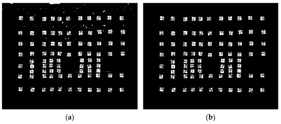
Figure 11. Threshold segmentation results: (a) Adaptive threshold processing; (b) Optimizing segmentation.

After segmenting all the reference point images, contour detection is used to determine the bounding rectangle for each reference point image, obtaining the reference point image areas from the original image. This concludes the process of reference point detection, with the outcomes displayed in Figure 12a. Once all the reference points are detected, a decoding function is applied to individually recognize each reference point image, with the final recognition results shown in Figure 12b. The image reveals that the majority of reference points are accurately detected, although a small number are missed as a result of insufficient data. However, the missed points are located at the edges of the model and do not affect the measurement of deformation in the core area of the roadway. After identifying the encoded reference points, the displacement of each reference point can be quickly calculated in subsequent processing.

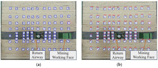
Figure 12. Mark point detection results: (a) Detection segmentation results; (b) Recognition results.

3.3.2. Stereo Calibration of Binocular Images

As shown in Figure 13, the original image captured by the binocular camera exhibits some distortion at the edges. First, the re-projection algorithm is used to correct the original distorted image. Then, the BOUGHT algorithm is applied for stereo rectification to achieve epipolar alignment of the images [51]. The BOUGHT algorithm is a boundary detection and region partitioning method based on image segmentation. The method is extensively utilized within the domain of image processing, notably in the disciplines of medical imaging and remote sensing, as well as across a spectrum of sophisticated image analysis applications.

Figure 13. Original binocular images captured.

As shown in Figure 14, the binocular images after distortion correction and epipolar alignment are presented. Compared to the original image, the edges, which were distorted, have been cropped out. The images are then reprojected onto the canvas, maintaining their original size. This correction ensures corresponding points in the left and right images are aligned along the same horizontal lines (epipolar lines), facilitating more accurate depth estimation and 3D reconstruction in later stages of processing. After stereo calibration, the epipolar lines in the left and right images are aligned, achieving coplanarity and horizontal alignment, which meets the requirements of the parallel stereo vision setup. This step provides a solid foundation for the next phase of stereo matching, where corresponding points between the two images can be accurately identified and used for 3D reconstruction.

Figure 14. Stereoscopic correction results.

3.3.3. Improved Stereo Matching Algorithm

Once stereo calibration is completed, the rectified stereo images are then processed by the stereo correspondence module, during which the disparity between the images from the left and right cameras is computed to produce the depth information map. Utilizing the depth map, the 3D coordinates of objects within the left camera’s coordinate framework can be determined. By examining the variations in the 3D coordinates of the measurement points, the deformation of the adjacent rock mass can be assessed.

This paper employs an improved stereo matching method to accomplish the matching task of left and right views. As shown in Figure 15, the stereo matching results are compared between the improved SGBM algorithm and the original SGBM algorithm. The four disparity maps can all fully present the object’s contours and depth information. The entire model is situated on the same plane and appears in the same color, indicating that it is relatively close to the camera, while the blue areas represent regions that are farther away from the camera. When the matching BlockSize varies, the details in the regions of the disparity map also change. As shown in Figure 15a–c, with an increase in the BlockSize, the incidence of empty (or hole) points within the disparity map undergoes a gradual reduction. The contours of the objects become more complete and clearer, and the disparity map results become smoother. But if the matching block is too large, it may reduce the original details of the object. As shown in Figure 15d, the disparity map processed by the improved stereo matching algorithm retains more noticeable details, with fewer hole points, and the contours and edges of the object are clearly visible.

Figure 15. Stereo matching results under different parameters. (a) BlockSize = 5; (b) BlockSize = 7; (c) BlockSize = 9; (d) Improved SGBM algorithm.

The comparison between the binocular vision system and total station measurements demonstrates that the proposed approach not only achieves high accuracy but also offers significant advantages in time efficiency. Once the binocular vision system is calibrated, each image acquisition and 3D reconstruction cycle can be completed within approximately 3–5 s, depending on image resolution and computing hardware. In contrast, total station measurements typically require several minutes to obtain and process comparable deformation data, particularly when multiple monitoring points are involved. Moreover, the improved stereo matching algorithm based on adaptive BlockSize optimization enhances computational efficiency by reducing redundant calculations in uniform texture regions, resulting in an overall processing speed improvement of approximately 25% compared to the standard SGBM method. These improvements enable near–real-time monitoring of roadway surrounding rock deformation, even under dynamic and variable underground conditions. Further optimization through parallel computation and hardware acceleration will be pursued to achieve fully real-time performance in resource-constrained mining environments.

4. Prediction Experiment

4.1. Dataset and Model Parameter Settings

Deformation and failure data pertaining to the surrounding rock, acquired through the application of a binocular vision algorithm, serve as the primary source for training the model. A dataset is constructed using the deformation amounts of the roadway roof and three landmark points located 15.0 cm and 30.0 cm above it, with the roadway roof deformation amount 1 as the X feature. In the simulation experiment, the binocular vision measurement method was used to collect 60 sets of data at each of the two key layers, A and B, resulting in a total of 120 datasets. These 120 datasets were randomly divided, with 80% allocated as the training dataset Y_h1 and the remaining 20% as the testing dataset Y_h2.

In the process of using RF regression model, it is necessary to adjust the model parameters to achieve optimal results. The study uses the number of decision trees (n_estimators) and the maximum depth of the decision trees (max_depth) in RF regression model as examples, applying the method of controlling variables. The selection of optimal parameter values is determined by the model’s efficacy on the validation set, with a focus on minimizing the Mean Squared Error (MSE).

Initially, establish constant starting values for the remaining parameters and evaluate the model’s efficacy across varying tree counts using the datasets Y_h1 and Y_h2. Figure 16 illustrates the variation curve of the mean squared error (MSE) for the model as the number of trees changes, as applied to the two datasets. As the number of trees increases, the MSE exhibits a downward trend, and ultimately, the error levels off at approximately 0.0064. At this point, the number of trees is approximately 180, and the model reaches its optimal performance. Hence, the n_estimators parameter for the model using the Y_h1 dataset is adjusted to 180. The model reaches convergence more rapidly on the Y_h2 dataset. When the number of decision trees reaches 120, the mean squared error begins to stabilize. Therefore, the n_estimators parameter for the model on the Y_h2 dataset is set to 120.

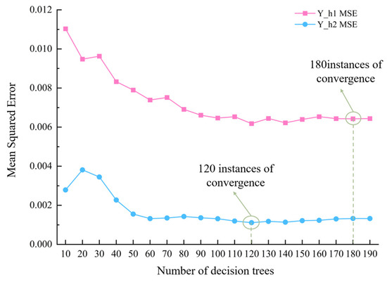
Figure 16. The results of Mean Square Error changing with the number of trees.

As shown in Figure 17, the mean squared error variation curve for the model on the two datasets with different tree depths is presented. As the tree depth increases, the mean squared error shows a decreasing trend, eventually converging to around 0.005. At this point, the tree depth is approximately 4, and the model reaches its optimal performance. Therefore, the max_depth parameter for the model on the Y_h1 dataset is set to 4. The model on the Y_h2 dataset converges more quickly, and when the depth reaches 3, the model achieves the minimum error. Therefore, the max_depth parameter for the model on the Y_h2 dataset is set to 3.

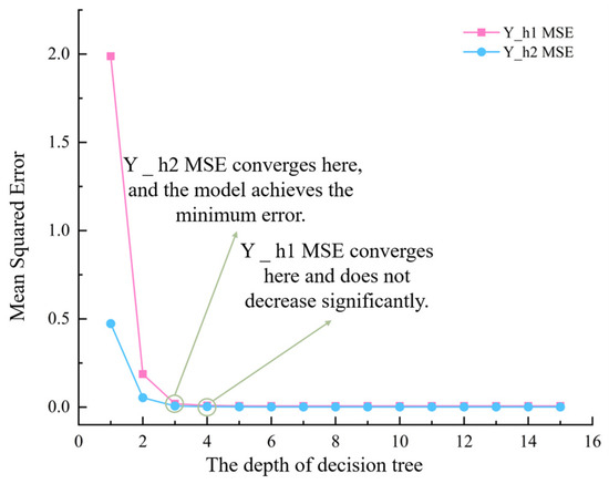
Figure 17. The results of mean square error changing with tree depth.

After analyzing the different parameters of the model, the final parameter settings are determined as shown in Table 3. The parameters min_samples_split and min_samples_leaf are also determined using this method.

Table 3. Key parameters of Random Forest algorithm.

Parameter	Implication	Y_h1 Parameter Setting	Y_h2 Parameter Setting
n_estimators	Number of decision trees	180	120
max_depth	Maximum depth of the tree	4	3
min_samples_split	The minimum number of samples required to segment internal nodes	2	2
min_samples_leaf	The minimum number of samples per leaf node	1	1

The performance of the GERF largely depends on data quality and model optimization. Effective feature engineering is essential to select highly relevant features such as depth information or texture features while minimizing the influence of noise. Additionally, model parameters, including the number of trees, tree depth, and splitting criteria, significantly affect the model’s generalization ability and must be carefully tuned to avoid overfitting. When the output of binocular vision such as 3D point clouds is used as input features, any inherent errors may propagate into the prediction results. For instance, depth deviations can lead to classification errors. Therefore, it is essential to jointly optimize the robustness of the binocular vision system (e.g., through illumination-invariant design) and the feature fusion strategy of the GERF. This coordinated approach ensures high precision and low latency throughout the data pipeline, thereby enhancing the overall reliability of the system.

4.2. Evaluation Metrics

The model is trained using the roof deformation and failure data X and the Y feature values at two different depths. The following assessment metrics are determined: Root Mean Squared Error (RMSE), R², and Cross-Validated Mean Squared Error (CV_MSE).

RMSE quantifies the average discrepancy between the values predicted by the model and the true values. It is the square root of the average of the squared errors. A lower RMSE signifies superior predictive accuracy of the model. The formula for computing RMSE is as follows:

$$RMSE=\sqrt{{\displaystyle \frac{1}{N}}{\displaystyle \sum _{i=1}^N{({\widehat{I}}_i-I_i)}^2}}$$

(6)

The determination coefficient, R², serves as a statistical metric for assessing the fit of a regression model. It varies between 0 and 1, where a higher value near 1 suggests a more accurate representation of the real data. The equation for computing R² is as follows:

$$R^2=1-{\displaystyle \frac{{\displaystyle \sum _{i=1}^N{({\widehat{I}}_i-I)}^2}}{{\displaystyle \sum _{i=1}^N{(I_i-\overline{I})}^2}}}$$

(7)

The calculation formula of CV_MSE is:

$$CV\_MSE={\displaystyle \frac{1}{k}}{\displaystyle \sum _{i=1}^n{(y_i-{\widehat{y}}_i)}^2}$$

(8)

5. Results and Analysis

5.1. Monitoring Results and Analysis

The difference map derived from the stereo correspondence algorithm can subsequently be employed to derive the three-dimensional coordinates of the reference points. By contrasting the three-dimensional coordinates of the reference points across various moments in time, the displacement of the fiducial points can be calculated, which is indicative of the deformation occurring in the surrounding rock in the roadway. To validate the accuracy of the stereo vision algorithm for the measurement of surrounding rock deformation and failure, this investigation conducts a comparative analysis of the outcomes with those derived from measurements utilizing a total station. In the loading experiment, the deep deformation of the roadway surrounding rock is relatively large, and it mainly occurs in the vertical direction, making it easier to obtain accurate results for comparison and analysis. Therefore, the movement of the marking points on the two key layers above the model roadway is selected to verify the accuracy of the stereo vision algorithm, as shown in Figure 18, referred to as Layer A and Layer B, respectively.

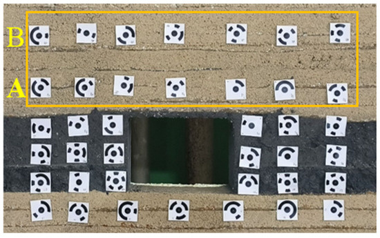
Figure 18. Selection of monitoring mark points of surrounding rock deformation.

The improved stereo vision algorithm has been employed to process the collected images of roadway surrounding rock deformation and failure, and the cumulative movement of the marker points on the surrounding rock surface is calculated. Meanwhile, the total displacement of the marker points is monitored and calculated using a total station. Finally, the deformation statistics for Layer A and Layer B of the surrounding rock are obtained for both methods.

As shown in Figure 19, it is evident that the deformation data derived from the stereo vision algorithm closely correspond to the measurements taken by the total station, with both sets of values aligning closely with the real experimental scenarios. The surrounding rock deformation and failure is greatest above the roadway roof, while the deformation of the surrounding rock farther away from the roadway is relatively smaller. Taking the total station monitoring outcomes as the precise benchmark, the mean measurement errors of the stereo vision algorithm for the deformation of the surrounding rock in Layer A and Layer B are determined to be 1.22 mm and 0.92 mm, respectively. In summary, the stereo vision-based roadway surrounding rock deformation and failure monitoring method can accurately measure the deformation of the surrounding rock, and in contrast to the total station method, it offers higher efficiency and a higher degree of automation.

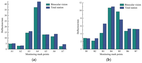
Figure 19. Comparison of surrounding rock deformation monitoring results. (a) A-layer deformation monitoring results; (b) B-layer deformation monitoring results.

5.2. Prediction Results and Analysis

After model training, the evaluation metric results of RF algorithm on the Y_h1 and Y_h2 datasets are shown in Table 4.

Table 4. Evaluation index results of model training.

Evaluating Indicator	Y_h1 Dataset	Y_h2 Dataset
RMSE	0.0164	0.0113
R2	0.8856	0.8356
CV_MSE	0.1281	0.1063

The findings from the model training exercise confirm that the GERF regression technique exhibits a high degree of predictive precision and robustness when applied to the Y_h1 and Y_h2 data matrices. In addition, the smaller CV_MSE, the better the model’s generalization ability on that dataset. The model’s RMSE on the Y_h1 dataset is only 0.0164, with an R² value of 0.8856 and a CV_MSE of 0.1281. This indicates that the model fits the test data on the Y_h1 dataset very well. The model’s RMSE on the Y_h2 dataset is only 0.0113, with an R² value of 0.8356 and a CV_MSE of 0.1063. This performance is even better than that on the Y_h1 dataset, which demonstrates that RF regression model has strong fitting capability for this type of data. The mechanism of the algorithm is proficient in delineating and extracting pertinent features from the training dataset, which culminates in the production of exemplary outcomes upon evaluation of the test set.

During the advancement of the physical similarity model working face, a total station was employed to monitor the displacement and deformation of the roadway roof, floor, and sidewalls in real time. The deformation measurements obtained from the total station were compared with the predictions generated by the GERF model to verify the accuracy of the predictive results. The model trained on the training dataset was used to perform predictive analysis on the test datasets Y_h1 and Y_h2. The fitting curves between the predicted values and the actual values are illustrated in Figure 20.

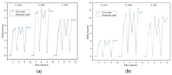
Figure 20. Model in the test set data fitting results. (a) Y_h1 prediction and fitting results on the test set; (b) Y_h2 prediction and fitting results on the test set.

Figure 20a depicts the efficacy of the model as applied to the Y_h1 test corpus. Y_h1A, Y_h1B, and Y_h1C represent the test data, which correspond to the actual displacement data of the three rows of markers at the roadway cover thickness of 4.5 m in the experiment. Y_h1A_Pre, Y_h1B_Pre, and Y_h1C_Pre denote the predictive outcomes yielded by the model for the respective test set datasets. The figure shows that the predicted values of the model fit very closely with the true values, with a consistent trend in the curve changes. This indicates that the model has effectively extracted the features from the dataset and can make accurate predictions on the test set data.

Figure 20b shows the model’s performance on the Y_h2 test set. Y_h2A, Y_h2B, and Y_h2C represent the test set data, while Y_h2A_Pre, Y_h2B_Pre, and Y_h2C_Pre are the corresponding predicted values. From the figure, it can be observed that the model also performs very well on the Y_h2 test set. The predicted value curves almost perfectly match the real value curves, with a fitting rate as high as 88.7%. The graphical correlation manifestly validates the efficacy of the model’s parameterization, affirming the robustness and precision of its predictive capabilities as evidenced by the alignment of the predicted and observed data trajectories.

The empirical validation of the trained RF regression model attests to its proficiency in delineating the quantitative correlation between rooftop deformation metrics and subsurface geological displacement data. This enables the forecasting of subsurface rock deformation and failure parameters exclusively from roof deformation observations.

The same dataset was used to predict the stability of roadway surrounding rock using ensemble learning methods: Adaboost, XGBoost, and Vision Transformer (ViT) [52,53].

Adaboost improves accuracy by focusing on hard-to-classify samples but is sensitive to noise and depends on weak learners. XGBoost enhances gradient boosting with regularization and parallelization, offering high performance but requiring complex tuning. ViT (Vision Transformer) uses self-attention on image patches for strong global feature extraction, excelling with big data but demanding high computational resources.

As shown in Table 5, Table 6 and Table 7, the GERF model exhibits slightly better fitting performance on datasets Y_h1 and Y_h2 compared to the Adaboost, XGBoost, and ViT models. Compared to the Adaboost model, it achieves up to a 25% reduction in root mean square error (RMSE), a maximum increase of 5% in the R² value, and up to a 12% reduction in cross-validation mean square error (MSE). Compared to the XGBoost model, the GERF model achieves up to a 33% reduction in root mean square error (RMSE), a maximum increase of 3% in the R² value, and up to a 15% reduction in cross-validation mean square error (MSE). Compared to the Vision Transformer model, it achieves up to an 18% reduction in RMSE, a maximum increase of 3.7% in the R² value, and up to an 8.7% reduction in cross-validation MSE. These results further validate that the GERF model has a strong fitting capability for this type of data.

Table 5. Evaluation index results of Adaboost model training.

Evaluating Indicator	Y_h1 Dataset	Y_h2 Dataset
RMSE	0.0202	0.0151
R2	0.8191	0.8127
CV_MSE	0.1421	0.1228

Table 6. Evaluation index results of XGBoost model training.

Evaluating Indicator	Y_h1 Dataset	Y_h2 Dataset
RMSE	0.0206	0.0147
R2	0.8341	0.8263
CV_MSE	0.1435	0.1212

Table 7. Evaluation index results of Vision Transformer model training.

Evaluating Indicator	Y_h1 Dataset	Y_h2 Dataset
RMSE	0.0194	0.0130
R2	0.8521	0.8311
CV_MSE	0.1392	0.1141

The GERF, Adaboost, XGBoost, and ViT models were evaluated using Precision, Specificity, Accuracy, Recall, and F-measure as performance metrics. The evaluation results for these four models are shown in the table.

As shown in Table 8, all models demonstrate good predictability during the training phase. Among them, the GERF model achieves the highest performance metrics. It can also be observed that the global and local evaluation metric averages of the Adaboost and XGBoost models are similar, indicating that their predictive performance for roadway surrounding rock stability is comparable. The VT model performs better than both the Adaboost and XGBoost models, but its overall evaluation metrics are slightly lower than those of the GERF model. Their model ranking scores are shown in Figure 21. The average values of these five evaluation metrics were scored, with the best-performing model among the four receiving 4 points, the next best 3 points, and so on, down to 1 point for the lowest-performing model. The results show that the GERF model achieved the most satisfactory predictive performance, earning the highest score of 17 points. Compared to the Adaboost, XGBoost, and ViT models, the GERF model’s overall performance improved by 7.82%, 8.68%, and 3.87%, respectively. This indicates that the predictive performance of the GERF model is superior to that of the Adaboost, XGBoost, and ViT models.

Table 8. The evaluation results of the three models in the test phase.

Model	Accuracy (%)	Specificity (%)	Precision (%)	Recall (%)	F-Measure (%)	Average (%)
GERF	83.037	83.425	81.328	81.015	85.315	82.824
ViT	80.631	76.541	81.614	82.014	73.983	78.9566
Adaboost	76.022	77.493	81.524	68.715	71.257	75.0022
XGBoost	75.521	77.231	79.656	66.254	72.014	74.1352

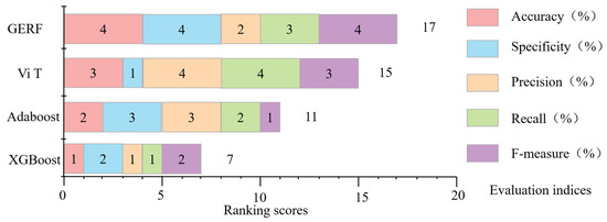
Figure 21. Ranking score of proposed model using test set.

5.3. Evaluation and Prospects

The results of this study show that the improved binocular vision system combined with the gradient-enhanced random forest (GERF) model can achieve accurate real-time monitoring of roadway surrounding rock deformation. Compared with traditional mine monitoring methods (such as laser scanning, total station and fiber optic sensors), the method in this paper effectively overcomes the limitations of high equipment cost, complex calibration and poor adaptability to low-light underground environments, and provides an economical, efficient, non-contact and real-time large-scale high-resolution spatial deformation data acquisition scheme. Similar to the fiber optic sensing technology developed by Chai et al. [23], this method can also continuously monitor deformation but has greater advantages in spatial resolution and coverage.

In terms of prediction, compared with stress and deformation prediction models such as PSO-ANFIS and ISVR proposed by Mahdevari et al. [27,28], the GERF-based model shows stronger generalization ability and stability. Traditional models mostly focus on single-point displacement prediction, while this study realizes spatiotemporal prediction of surface and deep deformation of surrounding rock by integrating multi-dimensional visualization data. Furthermore, the physical similarity model used is closer to the actual deformation situation on site, effectively bridging the gap between laboratory simulation and field observation by Zhu et al. [17].

The proposed method for monitoring and predicting roadway surrounding rock deformation based on an improved binocular vision system and a gradient-enhanced random forest (GERF) model has significant advantages. First, the method is low-cost and provides non-contact, real-time monitoring of large-scale, high-resolution spatial deformation data, significantly improving monitoring efficiency and accuracy. Second, combining a physical similarity model with machine learning enhances the accuracy and generalization ability of spatiotemporal deformation prediction, bridging the gap between laboratory simulations and complex field conditions. However, the method also has certain shortcomings and limitations. The binocular vision system is highly sensitive to lighting conditions and surface texture; low underground lighting and homogeneous surfaces may affect stereo matching accuracy, thus impacting monitoring effectiveness. Furthermore, the GERF model relies on a large amount of high-quality training data, making data acquisition and processing challenging and time-consuming. Interference factors in the mining environment, such as dust and vibration, may introduce measurement errors, affecting system stability and data reliability. In practical applications, the model’s generalization ability faces challenges, and prediction performance may decline under different geological conditions. The system’s reliance on high-performance computing and algorithm support also brings potential technical risks. The storage and real-time processing of high-frequency data also place high demands on equipment performance. Overall, while the method presented in this study has certain limitations, its comprehensive performance and innovation provide important technical support and a direction for the intelligent monitoring and prediction of surrounding rock deformation in mines.

This study demonstrates the significant potential of an intelligent monitoring and prediction method based on improved binocular vision and gradient-enhanced random forest (GERF) models in the field of surrounding rock deformation in mine roadways. In the future, this method is expected to further promote the development of intelligent and automated mining, achieving higher-precision, real-time monitoring and early warning of the underground environment. Scientifically, this research combines physical similarity modeling and machine learning to expand the theoretical framework of deformation prediction, providing new insights into the analysis of surrounding rock behavior in deep and complex geological environments. In terms of application, with the improvement of sensing technology and computing power, this method can be extended to more types of underground engineering and mining conditions, integrating multi-source sensor data to improve the robustness and adaptability of the system. Furthermore, combined with intelligent devices such as drones and robots, it can achieve broader autonomous monitoring and remote control in the future, contributing to the digital transformation of mine safety production and risk management.

6. Conclusions

This study developed a comprehensive deformation monitoring and prediction framework for deep soft-rock roadways by integrating binocular vision technology with machine learning. Through algorithmic innovation, physical modeling, and data-driven prediction, the research bridges the gap between laboratory-scale observation and real-time underground monitoring. The proposed system not only enhances the precision and robustness of deformation measurement but also expands the predictive capability of surrounding rock stability analysis. The main scientific and engineering conclusions are summarized as follows:

1. An improved Semi-Global Block Matching (SGBM) algorithm with an adaptive BlockSize mechanism was proposed, which dynamically adjusts the matching window based on image gradient and contrast. This enhancement significantly improves stereo-matching accuracy under the complex lighting and texture conditions typical of underground environments. A physical similarity-based experimental model using binocular vision was established to quantitatively analyze the deformation and failure characteristics of roadway surrounding rock. Validation against total station measurements demonstrated high reliability, with mean errors of 1.22 mm and 0.92 mm at different monitoring layers.

2. To predict deformation evolution, a Gradient-Enhanced Random Forest (GERF) model was developed and trained on datasets acquired through binocular vision monitoring. The model achieved an R² of 0.8856 for deep-level deformation prediction, surpassing AdaBoost, XGBoost, and ViT models by 7.82%, 8.68%, and 3.87%, respectively. The GERF model effectively integrates multi-dimensional visual data, enabling accurate spatiotemporal prediction of both surface and internal deformation in roadway surrounding rock. This provides a solid foundation for intelligent, data-driven monitoring and early warning in deep mining operations.

3. The proposed binocular vision monitoring system, integrated with the Gradient-Enhanced Random Forest (GERF) model, exhibits strong potential for practical application in underground mining operations. Its compact, non-contact design allows for seamless installation along roadway structures without interrupting production, while real-time monitoring enables continuous deformation tracking and early warning of instability. The system can be connected to existing mine safety management platforms for automated data exchange and visualization, reducing maintenance requirements and long-term costs compared with traditional sensors. In the future, integration with IoT frameworks and intelligent control systems will enable a closed-loop process of perception, prediction, and response, enhancing the safety and automation of deep mining operations. Continued research will focus on improving environmental adaptability, incorporating deep learning methods, and expanding multimodal datasets to strengthen system robustness and generalization.

References

- Kang, H.; Gao, F.; Xu, G.; Ren, H. Mechanical behaviors of coal measures and ground control technologies for China’s deep coal mines–A review. J. Rock Mech. Geotech. Eng. 2023, 15, 37–65. [Google Scholar] [CrossRef]
- Cai, X.; Yuan, J.; Zhou, Z.; Pi, Z.; Tan, L.; Wang, P.; Wang, S.; Wang, S. Effects of hole shape on mechanical behavior and fracturing mechanism of rock: Implications for instability of underground openings. Tunn. Undergr. Space Technol. 2023, 141, 105361. [Google Scholar] [CrossRef]
- Shan, P.; Meng, Z.; Lai, X.; Xue, X.; Li, C.; Wang, J.; Li, W.; Zhang, L.; Xi, B.; Jiang, H. A selection methodology on reasonable width of stabilized coal pillar for retracement channel in longwall working face. Front. Earth Sci. 2024, 12, 1430018. [Google Scholar] [CrossRef]
- Cui, F.; Zhang, S.; Lai, X.; Chen, J.; Jia, C.; Feng, G.; Sun, J. Coal and rock mass linkage induced impact mechanism and prevention and control rock burst in steeply-inclined and extremely-thick coal seam group. Chin. J. Rock Mech. Eng. 2023, 42, 3226–3241. [Google Scholar]
- Li, G.; Wan, Q.; Li, Z.; Yi, H.; Ren, F.; Chen, Z.; Liu, Y. A fractional-order creep model of water-immersed coal. Appl. Sci. 2023, 13, 12839. [Google Scholar]
- Jia, C.; Lai, X.; Cui, F.; Xu, H.; Zhang, S.; Li, Y.; Zong, C.; Luo, Z. Mining pressure distribution law and disaster prevention of isolated island working face under the condition of hard “umbrella arch”. Rock Mech. Rock Eng. 2024, 57, 8323–8341. [Google Scholar] [CrossRef]
- Xu, H.; Lai, X.; Shan, P.; Yang, Y.; Zhang, S.; Yan, B.; Zhang, Y.; Zhang, N. Energy dissimilation characteristics and shock mechanism of coal-rock mass induced in steeply-inclined mining: Comparison based on physical simulation and numerical calculation. Acta Geotech. 2023, 18, 843–864. [Google Scholar]
- Shan, P.; Meng, Z.; Xu, H.; Li, C.; Zhang, L.; Xi, B. Research on accurate recognition and refuse rate calculation of coal and gangue based on thermal imaging of transporting situation. Measurement 2025, 244, 116574. [Google Scholar] [CrossRef]
- Dai, L.; Feng, D.; Pan, Y.; Wang, A.; Ma, Y.; Xiao, Y.; Zhang, J. Quantitative principles of dynamic interaction between rock support and surrounding rock in rockburst roadways. Int. J. Min. Sci. Technol. 2025, 35, 41–55. [Google Scholar] [CrossRef]
- Wang, M.; Mitri, H.S.; Zhao, G.; Wang, S. Data-based assessment of rock strengths and cuttability using the monitored parameters while drilling, tunneling, and mining. Tunn. Undergr. Space Technol. 2025, 165, 106901. [Google Scholar] [CrossRef]
- Zhong, F.; Quan, C. Stereo-rectification and homography-transform-based stereo matching methods for stereo digital image correlation. Measurement 2021, 173, 108635. [Google Scholar] [CrossRef]
- Hong, P.; Ahn, C.W. Robust matching cost function based on evolutionary approach. Expert Syst. Appl. 2020, 161, 113712. [Google Scholar] [CrossRef]
- Mahdevari, S.; Khodabakhshi, M.B. A hierarchical local-model tree for predicting roof displacement in longwall tailgates. Neural Comput. Appl. 2021, 33, 14909–14928. [Google Scholar] [CrossRef]
- Zhu, Y.; Wang, S.; Liu, B.; Liu, X.; Kang, Y. Monitoring Technology of Surrounding Rock Deformation Based on IWFBG Sensing Principle and Its Application. Lithosphere 2023, 2023, lithosphere_2023_278. [Google Scholar] [CrossRef]
- Sadeghinezhad, E.; Siddiqui, M.A.Q.; Roshan, H.; Regenauer-Lieb, K. On the interpretation of contact angle for geomaterial wettability: Contact area versus three-phase contact line. J. Pet. Sci. Eng. 2020, 195, 107579. [Google Scholar] [CrossRef]
- Mo, J.; Dou, D.; Chen, C.; Liu, J. Research on alarm of coal content in gangue based on binocular vision and YOLACT segmentation network. Int. J. Coal Prep. Util. 2025, 45, 1737–1750. [Google Scholar] [CrossRef]
- Zhu, D.; Gao, L.; Ma, Q.; Zhuo, Z.; Li, Z. Research on the Deformation Mechanism and Control Technology of the Floor in Deep Soft Rock Roadway. Geofluids 2025, 2025, 5130542. [Google Scholar] [CrossRef]
- Zuo, J.; Ma, Z.; Xu, C.; Zhan, S.; Liu, H. Mechanism of principal stress rotation and deformation failure behavior induced by excavation in roadways. J. Rock Mech. Geotech. Eng. 2024, 16, 4605–4624. [Google Scholar] [CrossRef]
- Liu, G.; Kang, J.; Zhong, Z.; Bo, W.; Fan, H.; Yang, C. Laboratory Experiments and 3D DDA Numerical Simulations on Rockfall Movement Characteristics. Rock Mech. Rock Eng. 2025, 58, 9747–9769. [Google Scholar] [CrossRef]
- Du, Y.; Zhang, H.; Liang, L.; Zhang, J.; Song, B. Applications of machine vision in coal mine fully mechanized tunneling faces: A Review. IEEE Access 2023, 11, 102871–102898. [Google Scholar] [CrossRef]
- Han, Z.; Liu, H.; Guo, L.; Cheng, W.; Liang, J.; Chen, Z.; Guo, X.; Wang, H. A full-plane strain complex variable analytical model considering three-dimensional principal stress rotation and its engineering applications. Int. J. Coal Sci. Technol. 2025, 12, 88. [Google Scholar]
- Shen, Y.; Hou, B.; Wang, Y.; Pan, K. Mechanism and Control of Deformation and Failure of Mining Roadway in Thick Coal Seams Under Close Range Goaf. Energy Sci. Eng. 2025, 13, 2585–2601. [Google Scholar] [CrossRef]
- Chai, J.; Zhicheng, H.; Wulin, L.; Dingding, Z.; Jianfeng, Y.; Chenyang, M.; Gang, H.; Mingyue, W. The application of distributed fiber-optic sensing technology in monitoring the loose zone in the floor of stoping roadway. Rock Mech. Rock Eng. 2025, 58, 723–744. [Google Scholar]
- Liang, M.; Fang, X.; Song, Y.; Li, S.; Chen, N.; Zhang, F. Research on three-dimensional stress monitoring method of surrounding rock based on FBG sensing technology. Sensors 2022, 22, 2624. [Google Scholar] [CrossRef]
- Zhang, T.; Xu, Y.; Wei, C.; Su, H.; Feng, Y.; Yu, L. The influence of disturbance location and intensity on the deformation and failure of deep roadway surrounding rocks. Front. Mater. 2025, 12, 1550247. [Google Scholar] [CrossRef]
- Cheng, J.; Jiang, H.; Wang, D.; Zheng, W.; Shen, Y.; Wu, M. Analysis of position measurement accuracy of boom-type roadheader based on binocular vision. IEEE Trans. Instrum. Meas. 2024, 73, 5016712. [Google Scholar] [CrossRef]
- Mahdevari, S.; Khodabakhshi, M.B. A hybrid PSO-ANFIS model for predicting unstable zones in underground roadways. Tunn. Undergr. Space Technol. 2021, 117, 104167. [Google Scholar] [CrossRef]
- Mahdevari, S. Prediction of tailgate stability in mechanized longwall mines using an improved support vector regression model. Arab. J. Geosci. 2021, 14, 216. [Google Scholar] [CrossRef]
- Xu, H.; Li, K.; Shan, P.; Wu, X.; Zhang, S.; Wang, Z.; Liu, C.; Yan, Z.; Wu, L.; Wang, H. Automatic picking method for the first arrival time of microseismic signals based on fractal theory and feature fusion. Fractal Fract. 2025, 9, 679. [Google Scholar] [CrossRef]
- Ouyang, Z.; Li, G.; Wang, Q.; Yi, H.; Li, Z.; Shi, Q. An in-situ modification method for coal roadways with heightened burst risk. Front. Earth Sci. 2023, 11, 1128697. [Google Scholar] [CrossRef]
- Ji, Z.; Yi, H.; Li, G.; Liu, B.; Wu, Z. Numerical Implementation of the Barcelona Basic Model Based on Return-Mapping Integration. Appl. Sci. 2022, 12, 11933. [Google Scholar] [CrossRef]
- Zhong, Z.; Zhu, K.; Wang, N.; Li, L.; Li, Z. Quantifying crack and fractal features in multi-hole limestone combined with x-ray CT and machine learning. Bull. Eng. Geol. Environ. 2025, 84, 518. [Google Scholar] [CrossRef]
- Fu, Z.; Zheng, X.; Yan, Y.; Xu, X.; Zhou, F.; Li, X.; Zhou, Q.; Mai, W. The Evolution of Machine Learning in Large-Scale Mineral Prospectivity Prediction: A Decade Innovation (2016–2025). Minerals. 2025, 15, 1042. [Google Scholar] [CrossRef]
- Zhao, H.; Ma, X.; Fan, Y.; Dong, X.; Kang, Y.; Wen, P. Research on identification, separation and mechanism of soft and hard gangue from raw coal gangue via dual-energy X-ray based on machine learning. Int. J. Coal Prep. Util. 2025, 1–22. [Google Scholar] [CrossRef]
- Mohammed, B.; Hamza, C. A Robust Estimation of Blasting-Induced Flyrock Using Machine Learning Decision Tree Algorithms: Random Forest, Gradient Boosting Machine, and XGBoost. Min. Metall. Explor. 2025, 42, 1609–1624. [Google Scholar]
- Hassan, M.; Arman, H. Several machine learning techniques comparison for the prediction of the uniaxial compressive strength of carbonate rocks. Sci. Rep. 2022, 12, 20969. [Google Scholar] [CrossRef]
- Gao, G.; Wang, S.; Shuai, C. Optimization of greenhouse tomato localization in overlapping areas. Alex. Eng. J. 2023, 66, 107–121. [Google Scholar] [CrossRef]
- Rhodes, J.S.; Cutler, A.; Moon, K.R. Geometry-and accuracy-preserving random forest proximities. IEEE Trans. Pattern Anal. Mach. Intell. 2023, 45, 10947–10959. [Google Scholar]
- Sanchez, L.K.; Emery, X.; Seguret, S.A. Geostatistical modeling of Rock Quality Designation (RQD) and geotechnical zoning accounting for directional dependence and scale effect. Eng. Geol. 2021, 293, 106338. [Google Scholar] [CrossRef]
- Shan, P.; Yan, C.; Lai, X.; Sun, H.; Li, C.; Chen, X. Evaluation of real-time perception of deformation state of host rocks in coal mine roadways in dusty environment. Sustainability 2023, 15, 2816. [Google Scholar] [CrossRef]
- Ramirez-Hernández, L.R.; Rodríguez-Quinoñez, J.C.; Castro-Toscano, M.J.; Hernández-Balbuena, D.; Flores-Fuentes, W.; Rascon-Carmona, R.; Lindner, L.; Sergiyenko, O. Improve three-dimensional point localization accuracy in stereo vision systems using a novel camera calibration method. Int. J. Adv. Robot. Syst. 2020, 17, 1729881419896717. [Google Scholar] [CrossRef]
- Mulumba, D.M.; Liu, J.; Hao, J.; Zheng, Y.; Liu, H. Application of an optimized PSO-BP neural network to the assessment and prediction of underground coal mine safety risk factors. Appl. Sci. 2023, 13, 5317. [Google Scholar] [CrossRef]
- Tang, Y.; Zhou, H.; Wang, H.; Zhang, Y. Fruit detection and positioning technology for a Camellia oleifera C. Abel orchard based on improved YOLOv4-tiny model and binocular stereo vision. Expert Syst. Appl. 2023, 211, 118573. [Google Scholar] [CrossRef]
- Meng, N.; Bai, J.; Yoo, C. Failure mechanism and control technology of deep soft-rock roadways: Numerical simulation and field study. Undergr. Space 2023, 12, 1–17. [Google Scholar] [CrossRef]
- Karrari, S.S.; Heidari, M.; Khaleghi-Esfahani, M. New rock toughness index based on drilling and tensile strength by using entropy of decision tree and geotechnical analysis. Q. J. Eng. Geol. Hydrogeol. 2025, 58, qjegh2024-168. [Google Scholar] [CrossRef]
- Guo, Z.; Li, W.; He, M.; You, J.; Li, Y. Model test on failure mechanisms of deep high-stress soft rock roadways based on excavation compensation method. Eng. Fail. Anal. 2024, 160, 108161. [Google Scholar] [CrossRef]
- Jing, W.; Zhou, J.; Yuan, L.; Jin, R.; Jing, L. Deformation and failure mechanism of surrounding rock in deep soft rock tunnels considering rock rheology and different strength criteria. Rock Mech. Rock Eng. 2024, 57, 545–580. [Google Scholar]
- Lei, Y.; Wen, Z.; Wang, L.; Jiang, J.; Zuo, Y. Cascade rupture theory of coal and gas outbursts: A physics-based mathematical framework for catastrophic failure. Int. J. Rock Mech. Min. Sci. 2025, 195, 106309. [Google Scholar] [CrossRef]
- Xiong, X.; Ouyang, Y.; Dai, J.; Ling, Z. Analysis and control of self stable balance circle of surrounding rock of roadway in inclined coal seam. Appl. Math. Model. 2023, 124, 749–767. [Google Scholar] [CrossRef]
- Zeng, Q.; Xu, W.; Gao, K. Measurement method and experiment of hydraulic support group attitude and straightness based on binocular vision. IEEE Trans. Instrum. Meas. 2023, 72, 7502814. [Google Scholar] [CrossRef]
- Samek, W.; Montavon, G.; Lapuschkin, S.; Anders, C.J.; Müller, K.R. Explaining deep neural networks and beyond: A review of methods and applications. Proc. IEEE 2021, 109, 247–278. [Google Scholar] [CrossRef]
- Bouayach, N.; Kassou, F.; Rguig, M. 3D combined stratigraphy and geo-properties modeling using probabilistic machine learning. Eng. Geol. 2025, 357, 108387. [Google Scholar] [CrossRef]
- Yan, Z.; Chen, H.; Dong, X.; Zhou, K.; Xu, Z. Research on prediction of multi-class theft crimes by an optimized decomposition and fusion method based on XGBoost. Expert Syst. Appl. 2022, 207, 117943. [Google Scholar] [CrossRef]
Disclaimer/Publisher’s Note: The statements, opinions and data contained in all publications are solely those of the individual author(s) and contributor(s) and not of MDPI and/or the editor(s). MDPI and/or the editor(s) disclaim responsibility for any injury to people or property resulting from any ideas, methods, instructions or products referred to in the content. |
© 2025 by the authors. Licensee MDPI, Basel, Switzerland. This article is an open access article distributed under the terms and conditions of the Creative Commons Attribution (CC BY) license (https://creativecommons.org/licenses/by/4.0/).