Pairwise Coupling of Convolutional Neural Networks for the Better Explainability of Classification Systems

Abstract

Ensembling techniques are viewed as a promising machine learning tool to resolve issues arising from the monolithic nature of deep neural networks. In this paper, we consider pairwise coupling models built from neural networks, which is a special kind of ensemble. These models promise to provide much needed modularity in classification models employing deep networks. In order to be practical, pairwise coupling models have to have comparable memory and speed requirements to commonly used architectures. In this paper, we propose novel architectures that address this key problem of pairwise coupling models. We show that the classification accuracy of the resulting pairwise coupling models matches the original network, while exceeding the original network’s pairwise accuracy. The introduction of these pairwise models brings additional benefits. First, they allow for much less expensive uncertainty predictions. Secondly, their modularity allows for the fine-tuning of classification accuracy. Both of these benefits can be viewed as relating to the larger topic of improving the explainability as well as the modularity of deep neural networks.

1. Introduction

Deep convolutional neural networks [1] have emerged as a very powerful type of classification model that is finding applications across diverse fields. A typical neural network model has many millions of parameters embedded in a deep multilayer structure, making them very opaque classifiers whose inner workings are poorly understood. The lack of explainability of deep neural networks is viewed as a major weakness. However, one should note that explainability is a multifaceted phenomenon [2,3,4]. Let us consider several examples illustrating distinct viewpoints regarding explainability.

Deep neural networks are considered for use in scenarios that may result in fatalities. The severe malfunctioning of a system comprising a neural network, such as the unfortunate fatality caused by Uber Autonomous in Arizona, will have negative impacts on the public’s acceptance of AI technologies. Therefore, as well as for legal reasons, it is important to perform precise analyses, ideally with the identification of the root cause, of why such misprediction occurred. We call this requirement post hoc explicability. Such analysis may take many forms, e.g.:

• One may investigate which particular sample(s) in the training dataset inspired the network to make a prediction, an early example of which is [5], where the authors compared activations with those in the training dataset;
• One may be curious which part of the classified image led the CNN to make its classification decision—typically visualized using a heatmap, as in [6,7,8].

Another approach involves analyzing the inner workings of a neural network. An example of this is the interpretation of receptive fields of neurons, especially in early levels of deep networks [9]. It would be better still to have explainability in development, when one may use the insights provided about the classification system to change it in order to prevent possible malfunctions (mispredictions) during system deployment. However, the complete retraining of a large network is often too costly, especially since there is no guarantee that it will bring about the desired improvement. It is therefore desirable to only perform incremental improvement of the system, so that most of the training effort is retained. However, in standard neural networks, it is next to impossible to identify the subset of weights or the substructure of a large network that causes erroneous predictions. One solution would be establishing modularity in the classification system of the kind traditionally provided by ensembles in machine learning [10]. The absence of modularity in neural network has long been a recognized problem [11], but only recently have ensemble methods (with a mixture of experts [12]) found their place among industrial strength deep network systems [13].

Given the complex nature of explainability and its varied benefits, one may expect that engineering explainability into classification systems entails costs and poses hurdles during model development. In this paper, we examine these tradeoffs for a class of models constructed by means of pairwise coupling (an ensembling technique) from convolutional neural networks. The modularity of these models is especially suitable for studying explainability facets occurring when one restricts classification to a smaller subset of classes.

Medicine abounds with the need for explainable classification systems [14,15]. Let us describe a novel facet of explainability applicable in the medical field. Consider the case of a physician specialist who is being assisted by a system employing a convolutional neural network in diagnosis based on patient data (e.g., X-ray, MRI, or histology data). A convolutional neural network may arrive at a class prediction, while the specialist may feel that a different class is the correct one. Having narrowed the set of possibilities to this pair of classes (that preferred by the physician and that preferred by the network), it would be helpful for the classification system to provide the most precise prediction possible given that there are only two classification outcomes under consideration. An improvement is not possible in classification systems that exhibit independence of irrelevant alternatives (see Section 2.3) e.g., multinomial (softmax) regression, but if an improvement is possible, we say that a system exhibits enhanced pairwise explainability. This explainability is present in pairwise coupling models by design.

As we will show, pairwise coupling models can provide a benefit even in traditional explainability areas, namely uncertainty quantification [16,17]. Neural networks are affected by multiple randomness effects—from initialization through random dropout layers to the random ordering of training samples in batches. This prediction randomness is rarely explained to the end user, mainly because it would be costly to train many networks to obtain meaningful measures of randomness for the predictions. We shall say that systems providing an explanation of the stochasticity of predictions have uncertainty quantification.

The remainder of this paper is organized as follows. In Section 2, we will review principles of the pairwise coupling methodology. In Section 3, we will provide experimental details including a description of convolutional network architectures. In Section 4, we examine pairwise explainability through an evaluation of the pairwise accuracy of networks trained in a pairwise manner. In Section 5, we will evaluate multi-class accuracy of models built from networks trained in a pairwise manner. In Section 6, we will illustrate explainability in development using the concept of incremental improvement based on errors in the confusion matrix. In Section 7, we will illustrate uncertainty quantification by constructing many classification models in order to estimate the uncertainty of a prediction. Open research questions are discussed in the conclusion (Section 8).

2. Review of Pairwise Coupling

In this section, we outline the pairwise coupling classification methodology, proceeding from general definitions through historic motivation (SVM multi-class classification) to presenting state-of-the-art methods.

2.1. Classification Generalities

A (hard) classification problem can be defined as the search for a classifier function $f:X\to C$ mapping classified objects to a finite set C of dependent categories (classes) $C=\{C_1,\dots C_c\}$ [18]. When $c=2$, we speak of a binary classifier.

Often, one solves this problem by solving the soft classification problem first. This involves finding a posterior approximating predictor function $\tilde{f}:X\to {[0,1]}^c$, where c is the cardinality of the set C. If $\tilde{f}\left(x\right)=\left({\tilde{f}}_1\left(x\right),\dots ,{\tilde{f}}_c\left(x\right)\right)$, then the prediction is

$$f\left(x\right)=arg\underset{i\le c}{max}{\tilde{f}}_i\left(x\right).$$

The main reason for this detour is that it is convenient to optimize a smooth cost function of a parametric classification model using a gradient descent method. Such a gradient search underlies many machine learning methods, ranging from logistic regression to neural networks.

2.2. Motivation for Pairwise Coupling

A notable exception which does not fit the soft classification approach is the support vector machine model (SVM), a non-parametric classification technique very popular since the late 20th century [19,20]. The SVM model divides the feature space (or its higher-dimensional embedding via a kernel) into two subsets using a hyperplane, which is found by solving a quadratic programming problem. The innovative concept of bisection presented by SVM poses a problem for multi-class classifications problems (when $c>2$), because there is no obvious generalization of the quadratic programming problem to more than two classes. A methodology was thus developed that entails three major steps.

The first step is the adoption of one-on-one classification paradigm. This paradigm is characterized by requiring the creation of all possible pairwise SVM classifiers $f^{i,j}$ which are able to distinguish between the two classes $C_i$ and $C_j$ only. There are two immediate advantages to doing so. Since the model requires training only a portion of overall multiclass data, each pairwise classifier is easier to train. Moreover, each two-class dataset is more likely to be balanced, which would not be the case if one opted for a one-vs.-rest approach [21].

The second step is converting the hard classification model $f^{i,j}$ to a soft classification model ${\tilde{f}}^{i,j}$ by fitting a sigmoid function for each model. This was proposed in the work of J. Platt [22]. A subtle point in his approach was the adoption of uninformative priors on the labels, which avoids the overfitting problems associated with logistic regression.

The third step is known in the literature as the pairwise coupling approach [23,24], which converts the set of pairwise predictions provided by ${\tilde{f}}^{i,j}$ to a final multi-class posterior prediction.

2.3. Relationship Between Pairwise Likelihoods and Multi-Class Likelihoods

To understand pairwise coupling’s underlying principles, it is worthwhile to consider its “reverse” first. Suppose we are given a soft classifier which produces a class posterior vector $p\left(x\right)=\left(p_1\left(x\right),\dots ,p_c\left(x\right)\right)$ for a sample x. Given such a classifier and a pair of classes $i,j$ with $1\le i,j\le c$, one may construct a set of soft binary (i.e., two-class) classifiers $B_{ij}$, which we call the IIA restrictions of p.

This name is inspired by the axiom of independence of alternatives (IIA). In individual choice theory, the IIA axiom states that if an alternative x is preferred from a set T, and x is also an element of a subset S of T, then x should also be the preferred choice from S.

The IIA restriction classifier quantifies this principle. Its likelihoods are such that the relative likelihood ratio of classes i and j is the same as in the presence of the rest of the alternatives. Thus, the IIA restriction classifier $B_{ij}$ outputs the posterior distribution

$$\begin{array}{c}\hfill r_{ij}\left(x\right)=(\stackrel{p\left(C_i\right)}{\overbrace{{\displaystyle \frac{p_i\left(x\right)}{p_i\left(x\right)+p_j\left(x\right)}}}},\stackrel{p\left(C_j\right)}{\overbrace{{\displaystyle \frac{p_j\left(x\right)}{p_i\left(x\right)+p_j\left(x\right)}}}}),\end{array}$$

(1)

which is the unique two-class probability distribution on $\{C_i,C_j\}$ for which the relative likelihood of classes is $p_i\left(x\right)/p_j\left(x\right)$.

The ratios in Equation (1) may produce singular results if both $p_i\left(x\right)$ and $p_j\left(x\right)$ are simultaneously zero. We note that this singularity is avoided for a typical convolutional neural network, where the output of the softmax layer cannot produce a zero posterior for any class.

Thus, given multi-class prediction $p\left(x\right)$, we may construct the matrix of pairwise likelihoods:

$$\begin{array}{c}\hfill \mathbf{R}\left(x\right)=\left(\begin{array}{cccc}0& r_{12}\left(x\right)& \dots & r_{1c}\left(x\right)\\ r_{21}\left(x\right)& 0& \dots & r_{2c}\left(x\right)\\ ⋮& ⋮& \ddots & ⋮\\ r_{c1}\left(x\right)& r_{c-1,2}\left(x\right)& \dots & 0\end{array}\right),\end{array}$$

(2)

In this paper, we adopt the convention that on the diagonal of a matrix of pairwise likelihoods, there are always zeros. Then, the matrix of pairwise likelihoods has all entries in the interval $[0,1]$ and satisfies

$$\begin{array}{c}\hfill \mathbf{R}\left(x\right)+\mathbf{R}{\left(x\right)}^{\prime }=\left(\begin{array}{cccc}0& 1& \dots & 1\\ 1& 0& \dots & 1\\ 1& 1& \dots & 0\end{array}\right).\end{array}$$

(3)

An important fact is that the mapping $\Theta :p\left(x\right)\mapsto \mathbf{R}\left(x\right)$ does not lose any information.

Lemma 1.

The nonlinear mapping $p\left(x\right)\mapsto \mathbf{R}\left(x\right)$ is injective on the set of nonvanishing posteriors. In fact, if $p_i\left(x\right)\ne 0$ for all i, then it is possible to reconstruct $p\left(x\right)$ from any column or any row of the pairwise likelihood matrix.

Proof. 

See, e.g., [25] or [26]. □

2.4. Pairwise Coupling Methods

By a pairwise coupling method, we mean any method mapping the set of non-negative matrices $\mathbf{R}=\left(r_{ij}\right)$ satisfying (2) to the set of probability distributions on c classes. We say that a pairwise coupling method is regular if it inverts the map $\Theta$ from the matrix from multi-class posteriors $p\left(x\right)$ to the corresponding pairwise likelihood matrix $\mathbf{R}\left(x\right)$. Thus, if a regular pairwise coupling method is given a matrix of pairwise likelihoods constructed from a multi-class vector $\mathbf{p}$ by (1) and (2), the method should yield the original multi-class distribution.

The requirements for regular pairwise coupling are rather weak, because the mapping is prescribed only on the $n-1$ dimensional subspace of the $(n^2-n)/2$ dimensional parameter space of matrices satisfying (2). Therefore, there exist many different regular coupling methods.

In our work, we opted to use two regular pairwise coupling methods: the Wu–Ling–Wen method [27] and the Bayes covariant method [28]. The former is used in the popular LIBSVM library [29], while the latter has been proven to be a unique method satisfying additional hypotheses [28].

2.4.1. Wu–Ling–Weng Method

This method defines an optimization objective ${\delta }_2$ as follows:

$$\begin{array}{c}\hfill {\delta }_2:=\underset{\mathbf{p}}{min}\sum _{i=1}^k\sum _{j:j\ne i}{(r_{ij}{p}_j-r_{ji}{p}_i)}^2\end{array}$$

(4)

From the definition, it is immediately clear that the functional is non-negative. Moreover, it is zero on the image of map $\Theta :p\left(x\right)\mapsto \mathbf{R}\left(x\right)$ because from (1), we have

$$\begin{array}{c}\hfill r_{ij}{p}_j={\displaystyle \frac{p_i{p}_j}{p_i+p_j}}=r_{ji}{p}_i.\end{array}$$

(5)

Optimizing ${\delta }_2$ is also numerically efficient. Since the functional is a quadratic function of $p_i$, it is possible to reduce optimization to solving a set of linear equations.

2.4.2. Bayes Covariant Coupling

We proposed this method in our work [28]. The underlying idea is geometric. Let us call the variety of pairwise likelihood matrices (i.e., the image of map $\Theta$) the Bradley–Terry manifold. This method starts by mapping the matrix of pairwise likelihoods coordinatewise via

$$\begin{array}{c}\hfill {\theta }_{ij}:r_{ij}\mapsto log\left({\displaystyle \frac{1}{r_{ij}}}-1\right).\end{array}$$

(6)

In the new coordinate space, the Bradley–Terry manifold becomes a linear subspace, and the method is simply the orthogonal projection on the subspace.

2.4.3. Other Pairwise Coupling Methods

Let us briefly outline other coupling methods which have been proposed in the literature. In their comprehensive study of pairwise coupling Hastie and Tibshirani [23] introduce a coupling method that optimizes a functional derived from Kullback–Leibler divergence. The work of Zahorian and Nossair [30] on the classification of vowels using neural networks introduces another coupling method. Regular pairwise methods based on reverting map $\Theta$ in a columnwise manner have been proposed in [25,26]. Also, Wu, Lin, and Weng studied another coupling method based on a quadratic functional of posteriors [27].

2.5. Numerical Stability of Coupling Methods

Some coupling methods have numerically unstable behavior near the boundary of the space of possible pairwise likelihood matrices. For instance, Bayes covariant coupling suffers from this problem, since the mapping ${\theta }_{ij}$ in (6) is singular at the limit points zero and one.

In our work [28], we proposed two ways to deal with such instability:

• Start by choosing a small threshold $\frac{1}{2}\gg \tau >0$ and then force individual pairwise likelihoods $r_{ij}$ to lie in the interval $[\tau ,1-\tau ]$ by replacing them with $min(1-\tau ,max(\tau ,r_{ij}))$ if necessary;
• Choose a small threshold $\frac{1}{2}\gg \rho >0$ and remove from consideration any class c for which there is $c^{\prime }$ such that $r_{c{c}^{\prime }}<\rho$, i.e., remove all rows and columns from the pairwise likelihood matrix that correspond to such classes. Then apply the coupling method to the possibly smaller matrix of pairwise likelihoods. Finally, convert the posterior probability distribution to the full set of classes, for instance by extending with zero.

3. Methods

The models built by means of pairwise coupling need to be built from binary classifiers. In this section, we describe the dataset used, the three classes of convolutional neural networks employed as binary classifiers (micro-models, mini-models and macro-models), and the baseline multi-class networks which we used for comparison.

3.1. Dataset

We used the Fashion MNIST (FMNIST) dataset [31], which has been suggested [31] to be a better starting point for examining computer vision classification methods compared to the historically more popular MNIST dataset [32]. Moreover, the small size of this dataset resulted in short training times and thus in a low environmental impact for our experiments, an increasingly important societal consideration [33]. The overall training and test data sizes (60,000 and 10,000, respectively) are identical to those for MNIST. There are 10 classes, as shown in Table 1, evenly distributed in the dataset.

Table 1. Classes in the Fashion MNIST dataset.

Class	Description
0	T-shirt/top
1	trouser
2	pullover
3	dress
4	coat
5	sandal
6	shirt
7	sneaker
8	bag
9	ankle boot

3.2. Baseline Networks

To create our baseline model (model F in Figure 1), we used the Keras example CNN originally designed for the MNIST dataset (model M in Figure 1). The only structural difference is that we replaced dropout layers with batch normalization layers. There are two reasons for this adaptation:

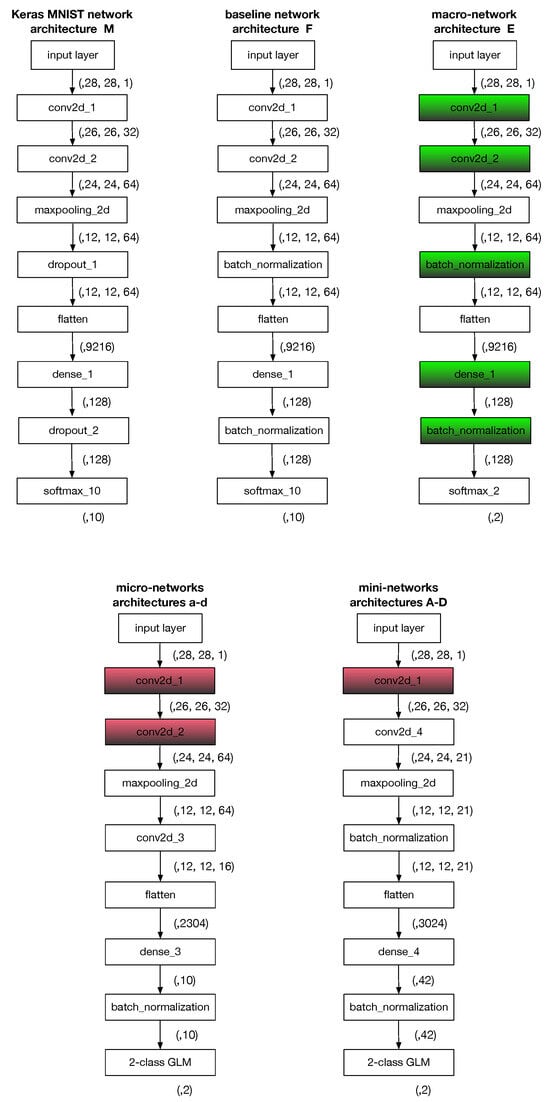
Figure 1. Schemas of feedforward CNN networks used for experiments, as well as the prototype network architecture from the Keras library. Tensor shapes below each box indicate the layer’s output shape. A red color indicates that layers’ weights were copied from the baseline model with the F architecture and were fixed throughout training. A green color indicates that the layers’ weights were copied from the baseline model with the F architecture but were not fixed during training. The final two-class general linear model (GLM) layer in architectures a–d, A–D was either logistic regression or the GLM model with a complementary log–log link function.

• The optimal probability of dropout may vary depending on the task. The values chosen for MNIST task may not be suitable for the Fashion MNIST task, and in this work we did not plan to perform any hyperparameter tuning.
• In the most recent survey on dropout methods [34], it is stated that dropout is not necessary for convolutional networks, and batch normalization is sufficient [35,36].

Overall, we trained 32 instances $F_0,\dots ,F_{31}$ of networks based on the F architecture, whose weights were later used in the initialization of the binary classifiers.

3.3. Architectures for Binary Models

We examined 9 different feed-forward architectures for binary models, which we describe in this section. Roughly in increasing size order, these architectures were micro-models (Section 3.3.1, see also architectures $a-d$ in Figure 1), mini-models (Section 3.3.2, architectures $A-D$ in Figure 1), and macro-models (Section 3.3.3, architecture E in Figure 1). For all of them, we trained 32 different networks, each partially initialized with the weights of the corresponding baseline network $F_i$ ($i\le 32$).

3.3.1. Binary Micro-Models

In Section 5, we will compare models built using pairwise coupling methods with the baseline model. It is desirable to use models with the same number of training parameters. Since a complete pairwise-coupled model requires 45 binary classifiers, individual binary classifiers have to be rather small. Namely, since the model G of the network has 1,200,650 parameters, individual binary classifiers should have ≈1,200,650/45 ≈ 26,681 parameters. It is quite challenging to achieve good performance with a convolutional network that small. A natural first step is to reduce the number of neurons (convolutions) in individual layers. However, based on our previous experience with share-none architectures [37], we felt that two additional alterations were needed:

• Reducing the number of 2D maps by using $1\times 1$ convolution.
• Sharing weights among individual pairwise classifiers. Thus, the first two layers of the binary classifiers had identical weights copied from the corresponding baseline network. These weights were not trainable.

The difference among the four variants of the micro-networks were as follows.

Networks a and b were trained with the softmax layers as the final layer. Networks c and d used the generalized linear model (GLM) model with a complementary log–log link function, which is considered more suitable in cases of non-symmetric distributions [38].

Networks a and c employed binary encoding of the dependent variable. Encoding of the dependent variable in networks b and d was altered to $ϵ$ instead of 0 and $1-ϵ$ instead of 1 with $ϵ=1/\left(\mathrm{size}\mathrm{of}\mathrm{the}\mathrm{training}\mathrm{set}\right)$ in an attempt to achieve the following:

• Mimicthe use of J. Platt’s uninformative prior in SVMs;
• Avoid numerical instabilities in pairwise coupling, as explained in Section 2.5.

3.3.2. Binary Mini-Models

A complete model built using pairwise coupling from binary micro-models has the same number of parameters as the baseline model. However, it is much easier to train, since each pairwise training dataset has $c/2=5$ times less data in it compared to the full Fashion MNIST dataset. We can roughly estimate that the complexity of training one epoch of a network is proportional to the product of the number of weights and the number of training samples. Since each pairwise micro-model has $c(c-1)/2$ fewer parameters, the complete arithmetical complexity to run the same number of epochs for all $c(c-1)/2$ networks is about $c/2=5$ times lower compared to the baseline model.

We therefore also investigated pairwise coupling models, termed mini-models, that have approximately the same total arithmetical training complexity as the baseline model, although they have more parameters. The underlying binary mini-networks have $c/2$ times more parameters than micro-networks, or equivalently, $(c-1)$ times fewer parameters than the baseline networks. Their architecture is shown in Figure 1.

Analogously to the case of micro-models, we used 4 flavors of this architecture. The models $A,B$ used softmax as the final layer, whereas the models $C,D$ used a complementary log–log GLM model. The models $A,C$ used standard binary encoding of the class variable, whereas the models $B,D$ used the same encoding as for the models $b,d$.

3.3.3. Binary Macro-Models

We also included models of type E, as shown in Figure 1, whose architecture is identical to the baseline model F except for the final layer, which is not a 10-class softmax layer, but rather a 2-class softmax layer. The models are initialized with the weights of the corresponding F model, but all weights are left trainable.

3.4. Evaluation Metrics

For evaluation, we used two metrics. First, the multi-class accuracy is defined as

$$\mathrm{Classification}\mathrm{accuracy}={\displaystyle \frac{\mathrm{Number}\mathrm{of}\mathrm{correctly}\mathrm{predicted}\mathrm{samples}}{\mathrm{Number}\mathrm{of}\mathrm{all}\mathrm{samples}}}.$$

We also used the pairwise accuracy metric. For a soft classifier which assigns posterior distribution $p\left(x\right)=(p_1,\dots ,p_K)$ over K classes, this is defined as the mean of the (multi-class) accuracies for IIA restrictions to all pairs of classes, as defined by (1).

3.5. Other Details

Multi-class networks were trained using a batch size of 128, whereas for binary models, we decreased the batch size to 32. The number of epochs was 12 in all cases.

In all cases, we used the AdaDelta stochastic gradient optimizer with standard settings and cross-entropy as the optimization criterion.

Finally, Table 2 shows the parameter counts for all networks used.

Table 2. Sizes of network architectures.

Architecture	Number of Prediction Classes	Total Parameters	Trainable Parameters	Non-Trainable Parameters
a, b	2	42,968	24,132	18,836
c, d	2	42,957	24,121	18,836
A, B	2	133,777	133,331	446
C, D	2	133,734	133,288	446
E	2	1,199,618	1,199,234	384
F	10	1,200,650	1,200,266	384

4. Evaluation of Pairwise Accuracy

In Section 1, we introduced the concept of pairwise explainability. This concept refers to the situation where we are confident that only two possible predictions are possible and we desire the best possible prediction by a convolutional neural network. Of course, one may obtain a two-class prediction by taking the IIA restriction of a multi-class classifier. But is it possible to obtain better results by training specialized binary networks on only two classes?

In this section, we present the answers to this question for the binary architectures described in Section 3.

4.1. Influence of Architecture

In Figure 2, we plot boxplots for the average pairwise performance over 32 training epochs for each architecture.

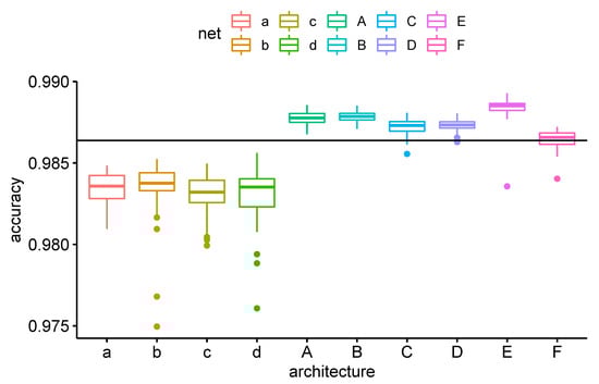
Figure 2. Average pairwise accuracy for architectures $a-d$ and $A-F$ over 32 trials. The horizontal line indicates the mean pairwise accuracy for the architecture F.

From this figure, we see the obvious trend that with increasing size, the convolutional networks perform better. The key point is that all mini-architectures $A-D$ (as well as the macro-architecture E) perform better than (the IIA restrictions of) the standard multi-class network (architecture F). On the other hand, all micro-networks of types $a-d$ perform worse than the multi-class network.

4.2. Detailed Performance by Pairs of Classes

We also plot the pairwise accuracy for each pair of classes in Figure 3. From this figure, it is clear that only a handful of pairs of classes show uneven performance among architectures:

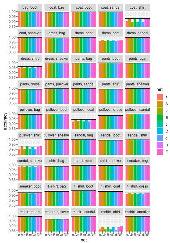
Figure 3. Average pairwise accuracy of individual architectures for all possible pairs of classes. The black horizontal line indicates the mean accuracy of architecture F.

• Coat/shirt;
• Dress/coat;
• Dress/shirt;
• Pullover/coat;
• Pullover/shirt;
• T-shirt/shirt.

Again, as observed above, it is the size of the architecture that is the primary factor affecting the pairwise accuracy. Moreover, the results strongly suggest that not all decision boundaries are equally difficult to find, and thus in multi-class pairwise-coupled models, varying learning capacity (i.e., the number of trainable parameters) is likely needed to construct an optimal two-class classifier.

5. Multi-Class Accuracy of Models Built via Pairwise Coupling

In the previous section, we concentrated on the question of whether pairwise accuracy can be improved by training a network with only two classes. We found that for mini-networks, the answer is yes. In this section, we investigate whether this improvement translates to better multi-class accuracy in pairwise coupling models. There is even the possibility that despite the inferior pairwise performance of micro-networks compared with the baseline model, using pairwise coupling may repair their pairwise mispredictions, and thus the multi-class models built from micro-networks using pairwise coupling could be more accurate that the baseline model. This effect, which we term coupling recovery, was examined based on synthetic datasets in [23,27].

5.1. Preliminaries

In order to build the multiclass models from pairwise ones, we need to take into account a couple of additional factors. The first is that in addition to architecture, one needs to choose a coupling method. As indicated in Section 2.4, we are going to use two coupling methods, namely the canonical Wu–Ling–Weng method and the Bayes covariant method. Additionally, the Bayes covariant method is not numerically stable, meaning that one needs to choose a way to avoid numerical singularities. We will use the first method outlined in Section 2.5. In order to do this, one needs to choose a threshold $\frac{1}{2}\gg \tau >0$, and we opted for the value $\tau ={10}^{-3}$. We illustrate the suitability of this value by plotting the accuracy of predictions for four different pairwise coupling models based on the A network architecture, as shown in Figure 4.

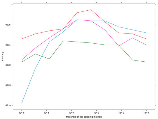
Figure 4. The accuracies of four different pairwise coupling models built from the A architecture and using the Bayes covariant coupling method with the given threshold $\tau$.

5.2. Statistical Analysis

Let us start by calculating the average multi-class accuracies for each architecture–coupling method pair, as shown in Table 3.

Table 3. Average multi-class accuracies of the models built from pairwise classifiers.

Network	Wu-Lin-Weng Method	Bayes Covariant Method
a	0.902	0.907
b	0.904	0.909
c	0.903	0.905
d	0.901	0.903
A	0.923	0.926
B	0.924	0.926
C	0.921	0.923
D	0.922	0.924
E	0.928	0.929

The mean multi-class accuracy of the baseline model is 0.923. which shows that only some mini-models may outperform the baseline. We evaluated paired t-tests and obtained the results shown in Table 4. (Note that although the t-test assumes normality, it is considered be robust, so we omitted normality testing.)

Table 4. Evaluation of t-tests comparing performance of a mini-model with the baseline multi-class model. Three asterisks in significance column indicate highly significant departure from the null hypothesis i.e., p-value $<0.001$.

Pair	Coupling Method	p-Value	Significance
A–F	Wu-Lin-Weng	0.8839
B–F	Wu-Lin-Weng	0.4295
A–F	Bayes covariant method	0.0001	***
B–F	Bayes covariant method	$9.2\times {10}^{-5}$	***
C–F	Bayes covariant method	0.3767
D–F	Bayes covariant method	0.7246

We conclude that mini-models A and B outperform, in a multi-class setting, the baseline network when the Bayes covariant pairwise coupling method is used. However, the effect size is small (<1%).

Finally, we visualized activations in the last convolutional layer of different network architectures. The results are shown in Figure 5. We can see that while saliency maps of mini-networks mirror those of the baseline network, micro-architecture saliency maps differ markedly.

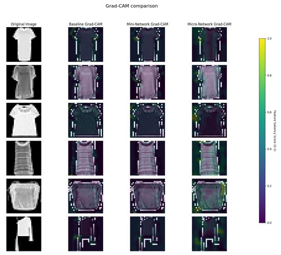
Figure 5. Saliency maps of different architectures computed using GradCAM.

6. Incremental Improvement

In this section, we investigate the possibility of correcting a poorly performing multi-class convolutional network. A standard way to understand the poor performance of a multi-class classifier is to construct the confusion matrix of predictions. For example, we trained a baseline classifier $F_0$, which had a confusion matrix, as shown in Table 5.

Table 5. The confusion matrix of the baseline classifier $F_0$ of type F.

	0	1	2	3	4	5	6	7	8	9
0	881	2	12	9	6	2	86	0	2	0
1	3	987	1	4	1	0	3	0	1	0
2	24	2	872	6	45	1	49	0	1	0
3	22	6	8	896	21	0	46	0	0	1
4	3	0	30	22	886	0	58	0	1	0
5	0	0	0	0	0	987	0	8	0	5
6	91	0	43	21	58	0	781	0	6	0
7	0	0	0	0	0	10	0	977	0	13
8	3	0	1	5	1	2	4	3	980	1
9	0	0	0	0	1	6	0	37	1	955

From this table, it is clear that the network makes most errors when confusing classes 0 and 6. We may try improving on the classification of an image x by applying a pairwise coupling method to the pairwise likelihood matrix $R^{\prime }\left(x\right)=\left(r_{ij}^{\prime }\left(x\right)\right)$, constructed as follows. Let $\left(p_0\left(x\right),\dots ,p_9\left(x\right)\right)$ be the prediction of $F_0$ and let $\left(q_0\left(x\right),q_6\left(x\right)\right)$ be the prediction of a binary classifier Q trained to distinguish classes 0 and 6. Then, we replace two entries of the pairwise likelihood matrix for $F_0$ by values provided by Q:

$$\begin{array}{c}\hfill r_{ij}^{\prime }\left(x\right)=\left\{\begin{array}{c}{q}_0\left(x\right)\mathrm{if}\mathrm{i}=0\mathrm{and}\mathrm{j}=6\hfill \\ q_6\left(x\right)\mathrm{if}\mathrm{i}=6\mathrm{and}\mathrm{j}=0\hfill \\ 0\mathrm{if}\mathrm{i}=\mathrm{j}\hfill \\ {\displaystyle \frac{p_i\left(x\right)}{p_i\left(x\right)+p_j\left(x\right)}}\mathrm{otherwise}\hfill \end{array}\right.\end{array}$$

(7)

We illustrate the results of such incremental improvements in Figure 6.

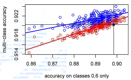
Figure 6. Plot of the multi-class versus the pairwise accuracy of 200 instances of incremental improvements given by (7). We used mini-networks of type A as the binary classifiers. A red color corresponds to the results for pairwise coupling with the Wu–Lin–Weng method, whereas a blue color stands for the Bayes covariant pairwise coupling. The black dot corresponds to the datum for the $F_0$ model. Linear regression lines are added.

We can conclude that even when Q has inferior pairwise accuracy to $F_0$, the coupling methods are able to increase the multi-class accuracy. The Bayes covariant method (red regression line in Figure 6) is slightly better than the Wu–Lin–Weng method (blue regression line) over the range of pairwise accuracies afforded by mini-networks of type A. However, the latter is more efficient in converting an increase in the pairwise accuracy to an increase in the multiclass accuracy. In fact, the linear regression model for the Wu–Lin–Weng method has an $R^2=0.81$, whereas it has an $R^2=0.46$ for the Bayes covariant method.

7. Likelihood Randomness Explainability

The incremental improvement achieved in the previous section was enabled by the inherent modularity of the pairwise coupling models. In this section, we examine another application of this modularity.

Neural networks are inherently random algorithms. Their predictions will vary if they are repeatedly trained. This fact is obvious to specialists, but is rarely conveyed to the end user. The primary obstacle is training cost. If it takes weeks to train a single deep neural network, it is utterly impractical to train, say, 100 different networks [39]. Other alternatives proposed for uncertainty quantification include using dropout [40] and Bayesian neural networks [41].

We will illustrate, based on an example from Fashion MNIST, that the problem of the expensive training of numerous copies of deep networks can be easily overcome using pairwise coupling models.

The image #142 (counted from 1) in the test set belongs to class 0 (t-shirt/top). It is shown in Figure 7.

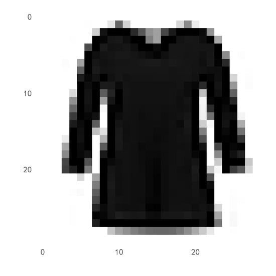
Figure 7. Image #142 from the Fashion MNIST test data set.

This image is correctly predicted to belong to class 0 by the network $A_1$, but is incorrectly predicted to belong to class 6 (shirt) by the network $A_2$. Both of them are quite sure, giving more than 95% likelihood for their prediction, as seen in Table 6.

Table 6. Predicted multi-class likelihoods for test image #142 by the networks $A_1$ and $A_2$.

Network	Class 0	Class 1	Class 2	Class 3	Class 4
$A_1$	9.53 × 10−1	2.04 × 10−8	1.13 × 10−2	1.55 × 10−5	1.53 × 10−8
$A_2$	5.58 × 10−8	3.59 × 10−2	9.41 × 10−6	5.06 × 10−10	4.80 × 10−11
Network	Class 5	Class 6	Class 7	Class 8	Class 9
$A_1$	1.63 × 10−2	3.16 × 10−11	4.69 × 10−4	9.91 × 10−4	4.83 × 10−8
$A_2$	1.63 × 10−9	9.82 × 10−1	6.88 × 10−7	2.32 × 10−9	6.27 × 10−9

The pairwise coupling approach allows one to create a vast number of new classifiers (more precisely, $2^{45}$) by bootstrapping pairwise predictions from either of the two pairwise likelihood matrices corresponding to the predictions of networks $A_1$ and $A_2$ and then applying a pairwise coupling method. We plot 100 samples for both pairwise coupling methods in Figure 8.

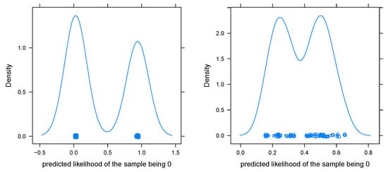
Figure 8. Predicted likelihoods of image #142 for 100 randomly recombined pairwise classifiers from networks $A_1$ and $A_2$. Left image: Using the Wu–Lin–Weng method; right image: using the Bayes covariant method.

The plots show that there is a significant difference between the Wu–Lin–Weng method and the Bayes covariant method. The former is strongly clustered in two clusters near 0 and 1, whereas the latter is much more uniformly distributed from 0.1 to 0.9. The natural assumption that the binary classifier for the pair 0/6 has a crucial influence on the multi-class posteriors is confirmed by plotting conditional density plots in Figure 9.

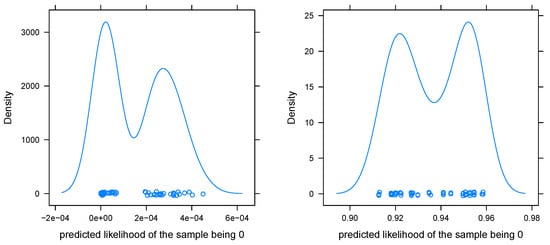
Figure 9. Predicted likelihoods of image #142 for 100 randomly recombined pairwise-classifiers from networks $A_1$ and $A_2$ using the Wu–Lin–Weng method. Left image: Conditioned on the 0/6 prediction being made by the IIA restriction of the network $A_1$; right image: conditioned on the 0/6 prediction being made by the IIA restriction of the network $A_2$.

Thus, the Wu–Lin–Weng method is very sensitive to the information provided by the critical binary classifier, whereas the Bayes covariant method tries to balance information from all binary classifiers. Both have their advantages. The former is more post hoc explicable, since a misprediction is likely caused by a single classifier. On the other hand, the latter is likely to be more precise, since it integrates information from many models.

8. Conclusions

In this paper, we have studied aspects of pairwise models built from convolutional neural networks. Let us summarize the key findings:

• We proposed a novel way to construct a pairwise coupling model by employing new architectures that match memory and compute the requirements of a standard convolutional network that match its accuracy;
• We showed that the models exhibit pairwise explainability;
• We demonstrated that pairwise coupling models allow for inexpensive uncertainty quantification when the Bayes covariant coupling method is used.

This establishes pairwise coupling as an additional ensembling method at the disposal of designers of real-world classification systems.

Let us discuss the finer details of our experiments.

8.1. Discussion of Experiments

The first observation is the failure to obtain better accuracy (pairwise or multi-class) with the pairwise coupling methodology using the same number of parameters as the baseline convolutional network. We hypothesize that this may be caused by allocating an equal number of parameters to pairwise classification tasks that vary significantly in difficulty (e.g., the shirt/t-shirt contrast seems to be by far the most difficult, see Figure 3 and Table 5). If that is so, then the success of the standard multi-class architecture (model F) suggests that CNNs are able to automatically allocate more capacity to the more challenging tasks. Another possible explanation is that in the presence of multiple classes, the convolutional network is able to learn multi-class features that go beyond those learnable in a two-class setting.

However, the subpar pairwise accuracy of micro-networks and subpar multi-class accuracy of micro-models should be contrasted with the success of mini-networks and mini-models. All mini-networks achieved higher pairwise accuracy than the baseline, and mini-models A and B (although not C and D) with the Bayes covariant method (but not the Wu–Lin–Weng method) obtained statistically significant improvements in performance over the baseline. Recall that the mini-models were designed to have approximately the same arithmetical complexity in training as the baseline. We would like to point out that there are likely additional performance advantages to using mini-models:

• The restricted memory size in graphics accelerators favors smaller models, and binary classifiers have fewer parameters than their multi-class equivalents;
• It is possible to train pairwise models in parallel without any communication among the computing nodes.

However, the accuracy improvements were modest for both mini-networks and mini-models, and thus by themselves are unlikely to attract adoption. On the other hand, there are two additional explainability attributes which are not present in commonly used CNN models.

The first is the ability to incrementally improve a multi-class classification system by incorporating specialized binary classifiers. It is even not mandatory that the specialized binary classifier outperforms the IIA restriction of the previous system. Our results show that diversity together with a pairwise coupling methodology is able to improve performance even in cases of subpar pairwise performance (cf. Figure 6). Thus, we were able to confirm the phenomenon of coupling recovery in a real data setting, which has previously been suggested in synthetic data experiments [23,27].

The second is the ability to gauge randomness in predicted likelihoods by building many more multi-class systems out of just a couple of pairwise-coupled systems (Section 7). In this case, we started to see a marked difference between the Wu–Lin-Weng coupling method and the Bayes covariant coupling method. The former seems to give too much confidence to a single pairwise decision, whereas the latter seems to take into account information from all decisions, leading to much more evenly distributed posteriors.

We also examined two methodological variations in creating pairwise coupling models. The first involved using a complementary log–log layer instead of softmax. As Figure 2 shows, this alternative led to inferior performance. The second involved using non-informative priors like the encoding of the dependent variable, and this step did not lead to noticeable improvements in classification accuracy.

8.2. Applications

Pairwise coupling models are best suited to situations where the number of classes under consideration changes frequently and it is expensive to retrain the full model. A prototypical example is an employee classification system based on biometrics (face images or voiceprints). A model based on pairwise coupling needs much less computing time to handle the addition of a new employee, and its modularity is well-suited to the reduction in the system size when an employee quits.

The uncertainty quantification provided by pairwise coupling, as demonstrated in Section 7, can be useful in fields such as the following:

• Autonomous driving;
• Healthcare and medical diagnosis;
• Climate science and environmental modeling;
• Finance and risk modeling.

8.3. Future Research

The main issue that hinders the adoption of pairwise coupling is the need to train multiple networks. This issue forced us to design specialized architectures of conventional neural networks so that the number of parameters of the pairwise model was comparable to that of the benchmark network. The severity of this problem increases with the number of classes K, since the number of pairwise models grows quadratically with K. Resolving this issue is the key step towards the broader adoption of pairwise classification models.

One solution is the adoption of the so-called arboreal coupling methods, for which the number of required models grows linearly. These were formalized in the preliminary work [42]. However, these arboreal coupling techniques do not exhaust approaches achieving linear growth in complexity. Moreover, they are non-canonical, so they require potentially expensive model selection. Therefore, finding optimal coupling techniques in the context of deep learning remains an open problem.

References

- LeCun, Y.; Bengio, Y.; Hinton, G. Deep Learning. Nature 2015, 521, 436–444. [Google Scholar] [CrossRef]
- Ibrahim, R.; Shafiq, M.O. Explainable convolutional neural networks: A taxonomy, review, and future directions. ACM Comput. Surv. 2023, 55, 1–37. [Google Scholar] [CrossRef]
- Zhang, Y.; Tiňo, P.; Leonardis, A.; Tang, K. A survey on neural network interpretability. IEEE Trans. Emerg. Top. Comput. Intell. 2021, 5, 726–742. [Google Scholar] [CrossRef]
- Vonder Haar, L.; Elvira, T.; Ochoa, O. An analysis of explainability methods for convolutional neural networks. Eng. Appl. Artif. Intell. 2023, 117, 105606. [Google Scholar] [CrossRef]
- Krizhevsky, A.; Sutskever, I.; Hinton, G.E. Imagenet classification with deep convolutional neural networks. In Proceedings of the 26th International Conference on Neural Information Processing Systems—NIPS’12, Lake Tahoe, NV, USA, 3–6 December 2012; Curran Associates Inc.: Red Hook, NY, USA, 2012; Volume 1, pp. 1097–1105. [Google Scholar]
- Zhou, B.; Khosla, A.; Lapedriza, A.; Oliva, A.; Torralba, A. Learning deep features for discriminative localization. In Proceedings of the IEEE Conference on Computer Vision and Pattern Recognition, Las Vegas, NV, USA, 27–30 June 2016; pp. 2921–2929. [Google Scholar]
- Selvaraju, R.R.; Das, A.; Vedantam, R.; Cogswell, M.; Parikh, D.; Batra, D. Grad-CAM: Why did you say that? arXiv 2016, arXiv:1611.07450. [Google Scholar]
- Ribeiro, M.T.; Singh, S.; Guestrin, C. “ Why should I trust you?” Explaining the predictions of any classifier. In Proceedings of the 22nd ACM SIGKDD International Conference on Knowledge Discovery and Data Mining, San Francisco, CA, USA, 13–17 August 2016; pp. 1135–1144. [Google Scholar]
- Zeiler, M.D.; Fergus, R. Visualizing and understanding convolutional networks. In Proceedings of the European Conference on Computer Vision, Zurich, Switzerland, 6–12 September 2014; Springer: Cham, Switzerland, 2014; pp. 818–833. [Google Scholar]
- Dietterich, T.G. Ensemble methods in machine learning. In Proceedings of the International Workshop on Multiple Classifier Systems, Cagliari, Italy, 21–23 June 2000; Springer: Berlin/Heidelberg, Germany, 2000; pp. 1–15. [Google Scholar]
- Caelli, T.; Guan, L.; Wen, W. Modularity in neural computing. Proc. IEEE 1999, 87, 1497–1518. [Google Scholar] [CrossRef]
- Jacobs, R.A.; Jordan, M.I.; Nowlan, S.J.; Hinton, G.E. Adaptive Mixtures of Local Experts. Neural Comput. 1991, 3, 79–87. [Google Scholar] [CrossRef]
- Liu, A.; Feng, B.; Xue, B.; Wang, B.; Wu, B.; Lu, C.; Zhao, C.; Deng, C.; Zhang, C.; Ruan, C.; et al. Deepseek-v3 technical report. arXiv 2024, arXiv:2412.19437. [Google Scholar]
- Zeineldin, R.A.; Karar, M.E.; Elshaer, Z.; Coburger, J.; Wirtz, C.R.; Burgert, O.; Mathis-Ullrich, F. Explainability of deep neural networks for MRI analysis of brain tumors. Int. J. Comput. Assist. Radiol. Surg. 2022, 17, 1673–1683. [Google Scholar] [CrossRef]
- Yu, L.; Xiang, W.; Fang, J.; Phoebe Chen, Y.P.; Zhu, R. A novel explainable neural network for Alzheimer’s disease diagnosis. Pattern Recognit. 2022, 131, 108876. [Google Scholar] [CrossRef]
- Kabir, H.D.; Khosravi, A.; Hosen, M.A.; Nahavandi, S. Neural network-based uncertainty quantification: A survey of methodologies and applications. IEEE Access 2018, 6, 36218–36234. [Google Scholar] [CrossRef]
- Gawlikowski, J.; Tassi, C.R.N.; Ali, M.; Lee, J.; Humt, M.; Feng, J.; Kruspe, A.; Triebel, R.; Jung, P.; Roscher, R.; et al. A survey of uncertainty in deep neural networks. Artif. Intell. Rev. 2023, 56, 1513–1589. [Google Scholar] [CrossRef]
- James, G.; Witten, D.; Hastie, T.; Tibshirani, R. An Introduction to Statistical Learning: With Applications in R; Springer Publishing Company: New York, NY, USA, 2014. [Google Scholar]
- Cortes, C.; Vapnik, V. Support-vector networks. Mach. Learn. 1995, 20, 273–297. [Google Scholar] [CrossRef]
- Vapnik, V. The Nature of Statistical Learning Theory; Springer: Berlin/Heidelberg, Germany, 1996. [Google Scholar]
- Mayoraz, E.N. Multiclass Classification with Pairwise Coupled Neural Networks or Support Vector Machines. In Proceedings of the Artificial Neural Networks—ICANN 2001, Vienna, Austria, 21–25 August 2001; Dorffner, G., Bischof, H., Hornik, K., Eds.; Springer: Berlin/Heidelberg, Germany, 2001; pp. 314–321. [Google Scholar]
- Platt, J.C. Probabilies for SV machines. In Proceedings of the Advances in Large Margin Classifiers, Breckenridge, CO, USA, 1–3 December 1998; MIT Press: Cambridge, MA, USA, 2000; pp. 61–74. [Google Scholar]
- Hastie, T.; Tibshirani, R. Classification by pairwise coupling. Ann. Statist. 1998, 26, 451–471. [Google Scholar] [CrossRef]
- Quost, B.; Destercke, S. Classification by pairwise coupling of imprecise probabilities. Pattern Recognit. 2018, 77, 412–425. [Google Scholar] [CrossRef]
- Šuch, O.; Beňuš, Š.; Tinajová, A. A new method to combine probability estimates from pairwise binary classifiers. In Proceedings of the Information Technologies–Applications and Theory, ITAT 2015, Slovensky Raj, Slovakia, 17–21 September 2015; pp. 194–199. [Google Scholar]
- Price, D.; Knerr, S.; Personnaz, L.; Dreyfus, G. Pairwise Neural Network Classifiers with Probabilistic Outputs. In Advances in Neural Information Processing Systems 7; Tesauro, G., Touretzky, D., Leen, T., Eds.; MIT Press: Cambridge, MA, USA, 1995; pp. 1109–1116. [Google Scholar]
- Wu, T.F.; Lin, C.J.; Weng, R.C. Probability Estimates for Multi-class Classification by Pairwise Coupling. J. Mach. Learn. Res. 2004, 5, 975–1005. [Google Scholar]
- Šuch, O.; Barreda, S. Bayes covariant multi-class classification. Pattern Recognit. Lett. 2016, 84, 99–106. [Google Scholar] [CrossRef]
- Chang, C.C.; Lin, C.J. LIBSVM: A Library for Support Vector Machines. ACM Trans. Intell. Syst. Technol. 2011, 2, 27:1–27:27. [Google Scholar] [CrossRef]
- Zahorian, S.A.; Nossair, Z.B. A partitioned neural network approach for vowel classification using smoothed time/frequency features. IEEE Trans. Speech Audio Process. 1999, 7, 414–425. [Google Scholar] [CrossRef]
- Xiao, H.; Rasul, K.; Vollgraf, R. Fashion-MNIST: A Novel Image Dataset for Benchmarking Machine Learning Algorithms. arXiv 2017, arXiv:1708.07747. [Google Scholar] [CrossRef]
- LeCun, Y.; Cortes, C. MNIST Handwritten Digit Database. 2010. Available online: http://yann.lecun.com/exdb/mnist/ (accessed on 1 April 2019).
- Strubell, E.; Ganesh, A.; McCallum, A. Energy and Policy Considerations for Deep Learning in NLP. arXiv 2019, arXiv:1906.02243. [Google Scholar] [CrossRef]
- Labach, A.; Salehinejad, H.; Valaee, S. Survey of Dropout Methods for Deep Neural Networks. arXiv 2019, arXiv:1904.13310. [Google Scholar] [CrossRef]
- Ioffe, S.; Szegedy, C. Batch Normalization: Accelerating Deep Network Training by Reducing Internal Covariate Shift. In Proceedings of the 32nd International Conference on Machine Learning, Lille, France, 7–9 July 2015; Bach, F., Blei, D., Eds.; Volume 37, pp. 448–456. [Google Scholar]
- He, K.; Zhang, X.; Ren, S.; Sun, J. Deep Residual Learning for Image Recognition. In Proceedings of the IEEE Conference on Computer Vision and Pattern Recognition (CVPR), Las Vegas, NV, USA, 27–30 June 2016. [Google Scholar]
- Šuch, O.; Tinajová, A.; Kontšek, M. Neural pairwise classification models created by ignoring irrelevant alternatives. In Proceedings of the ITAT 2015: Information Technologies–Applications and Theory, Donovaly, Slovakia, 20–24 September 2019. [Google Scholar]
- Piegorsch, W.W. Complementary Log Regression for Generalized Linear Models. Am. Stat. 1992, 46, 94–99. [Google Scholar] [CrossRef]
- Lakshminarayanan, B.; Pritzel, A.; Blundell, C. Simple and scalable predictive uncertainty estimation using deep ensembles. In Proceedings of the Advances in Neural Information Processing Systems NIPS’17, Long Beach, CA, USA, 4–9 December 2017; pp. 6405–6416. [Google Scholar]
- Gal, Y.; Ghahramani, Z. Dropout as a bayesian approximation: Representing model uncertainty in deep learning. In Proceedings of the International Conference on Machine Learning, PMLR, New York, NY, USA, 19–24 June 2016; pp. 1050–1059. [Google Scholar]
- Kendall, A.; Gal, Y. What uncertainties do we need in bayesian deep learning for computer vision? In Proceedings of the Advances in Neural Information Processing Systems NIPS’17, Long Beach, CA, USA, 4–9 December 2017; pp. 5580–5590. [Google Scholar]
- Šuch, O.; Novotný, P.; Haidar, A. New Bayes covariant coupling methods for adapting to change of priors in one-vs-one classification. J. Classif. 2025; under review. [Google Scholar]
Disclaimer/Publisher’s Note: The statements, opinions and data contained in all publications are solely those of the individual author(s) and contributor(s) and not of MDPI and/or the editor(s). MDPI and/or the editor(s) disclaim responsibility for any injury to people or property resulting from any ideas, methods, instructions or products referred to in the content. |
© 2025 by the authors. Licensee MDPI, Basel, Switzerland. This article is an open access article distributed under the terms and conditions of the Creative Commons Attribution (CC BY) license (https://creativecommons.org/licenses/by/4.0/).