Face and Voice Recognition-Based Emotion Analysis System (EAS) to Minimize Heterogeneity in the Metaverse

Abstract

The metaverse, where users interact through avatars, is evolving to closely mirror the real world, requiring realistic object responses based on users’ emotions. While technologies like eye-tracking and hand-tracking transfer physical movements into virtual spaces, accurate emotion detection remains challenging. This study proposes the “Face and Voice Recognition-based Emotion Analysis System (EAS)” to bridge this gap, assessing emotions through both voice and facial expressions. EAS utilizes a microphone and camera to gauge emotional states, combining these inputs for a comprehensive analysis. It comprises three neural networks: the Facial Emotion Analysis Model (FEAM), which classifies emotions using facial landmarks; the Voice Sentiment Analysis Model (VSAM), which detects vocal emotions even in noisy environments using MCycleGAN; and the Metaverse Emotion Recognition Model (MERM), which integrates FEAM and VSAM outputs to infer overall emotional states. EAS’s three primary modules—Facial Emotion Recognition, Voice Emotion Recognition, and User Emotion Analysis—analyze facial features and vocal tones to detect emotions, providing a holistic emotional assessment for realistic interactions in the metaverse. The system’s performance is validated through dataset testing, and future directions are suggested based on simulation outcomes.

1. Introduction

The concept of the metaverse, where individuals use their avatars to enjoy leisure and work in a virtual world, has become deeply ingrained in our society. The creation of avatars using personal photos is no longer a novel technology, and virtual showcases have become commonplace. Consequently, it has become important for objects in a virtual environment to react as if they were real, minimizing the disparity between virtual and real-world environments. Although emotion research based on voice and facial expressions has been ongoing even before the metaverse, the emotional states being assessed are often fragmented. While the development of eye-tracking, hand-tracking, and other technologies that transfer physical movements into virtual environments is ongoing, research on emotions remains fragmented due to the complexity of the environment. Accurate analysis of emotions is crucial for ensuring that objects in the metaverse interact with real-world entities in a more natural manner. Therefore, this study proposes the “Face and Voice Recognition-based Emotion Analysis System (EAS) to Minimize Heterogeneity in the Metaverse.” The system analyzes the user’s emotional state by simultaneously recognizing their voice and facial expressions. The EAS uses a microphone and camera to analyze the user’s voice and expressions and combines these inputs to determine the user’s overall emotional state. This paper aims to study three neural networks to develop the EAS. First, the Facial Emotion Analysis Model (FEAM) is designed to classify human expressions into seven emotions using facial landmarks, and a training dataset is generated to verify whether emotions can be accurately assessed from facial expressions. Second, the Voice Sentiment Analysis Model (VSAM) is designed to recognize emotions from the human voice. To improve accuracy, a model called MCycleGAN is proposed to extract voice data in noisy environments. Finally, the Metaverse Emotion Recognition Model (MERM) is designed to infer the overall emotional state of the speaker by combining the results of FEAM and VSAM. This paper is structured as follows: Section 2 discusses previous research on emotion analysis using voice and video recognition. Section 3 explains the structure and logical design of the proposed EAS. Section 4 presents the training and testing of the neural networks used in each module of EAS using public datasets to verify the system’s ability to recognize emotions at a level comparable to that of humans. Section 5 provides a summary of the proposed EAS and discusses future directions based on simulation results.

2. Related Works

2.1. Neural Network Models for Facial Emotion Analysis

Facial landmarks can provide various information about a person’s face. There are existing studies that classify human facial expressions using landmarks. In one study, the distances between facial landmarks were calculated to extract features and analyze relationships, classifying expressions into five categories [1]. Another study proposed an algorithm that utilizes a landmark-based ensemble network to classify expressions. This method uses landmark information from facial images to classify expressions into four emotional states through ensemble learning [2]. Various methods for extracting landmarks, which involve obtaining coordinates at specific locations on the face, have been researched. Extracting landmarks enables the recognition of faces in videos, which forms the foundation for technologies such as automatic facial focusing during video recording, detecting facial temperatures with thermal cameras, and inferring emotions from facial expressions [3].

With recent advances in deep learning, the performance of facial feature point detection methods has significantly improved. Although the heatmap regression approach is widely used as an efficient and powerful method, it has certain limitations. To address these, a method combining integral regression with the heatmap regression approach was proposed, which greatly improved landmark detection performance [4]. For real-time operation on mobile devices, a method was suggested to implement deep learning-based facial detection and facial landmark algorithms on mobile platforms without significantly altering the deep network structures originally designed for desktops [5].

There have been various prior studies on emotion classification through facial expressions using CNNs. One study focused on the theme of emotion and healing, recognizing users’ expressions using deep learning, and playing music to amplify the emotion corresponding to the detected expression. This study implemented a two-layer model based on the MNIST model, classifying expressions into three categories: happiness, sadness, and surprise [6]. Another study using CNNs addressed the limitations of existing expression databases by proposing a model that classifies expressions into ‘neutral’, ‘happy’, ‘sad’, ‘angry’, ‘surprised’, and ‘disgusted’ using high-quality, diverse databases [7].

To compare the predictive performance of various CNN architectures, a study analyzed the performance of AlexNet, GoogLeNet, VGGNet, and ResNet. Each model was trained for 100 epochs, with accuracy assessed at each epoch. The results indicated that accuracy tends to increase as the depth of the CNN architecture increases [8]. There is also research on developing a new small-scale deep convolutional neural network model to classify small datasets of low-resolution images. This model uses only a fraction of the memory compared to existing deep convolutional neural networks but produces very similar results on the FER2013 and FERPlus datasets [9]. These studies demonstrate that the optimal model structure may vary depending on the resolution of the input data, the size of the dataset, and the labels to be classified.

2.2. Neural Network Models for Voice Emotion Analysis

There is a Wiener filtering method that removes noise frequency bands while retaining the frequency bands of the sound to eliminate noise. However, it is challenging to remove all types of noise encountered in real-world scenarios using the Wiener filtering method alone. Consequently, recent studies have actively explored noise reduction using deep learning models. For instance, by training an autoencoder with noise, the model can extract noise features from noisy speech and then restore and remove noise from the original speech data [10].

A study demonstrated that CNNs could be used to distinguish between speech and non-speech segments in human voice data, thereby eliminating unnecessary voice signals [11]. Although deep learning models have shown promising results in the field of noise reduction, they are noted for being vulnerable to untrained noises. A GAN-based generative model trained for noise reduction has been shown to perform better at removing untrained noise [12].

The Speech Enhancement Generative Adversarial Network (SEGAN) was the first GAN-based deep learning model to demonstrate its effectiveness in the field of noise reduction [7]. The GAN-based deep learning model SEcGAN outperformed the traditional STSA-MMSE (short-time spectral amplitude minimum mean square error) algorithm [13].

In the field of Image-to-Image Translation, classical methods require training data to be paired, but collecting paired training data is often very costly. CycleGAN introduces the addition of a reverse generator to a conventional GAN, allowing for the use of unpaired training data [14]. Although the original CycleGAN was designed for image data transformation, it can also be applied to voice data by converting the voice into a spectrogram, allowing it to be processed as an image [15].

In standard GANs, Cross Entropy loss is typically used as the discriminator’s loss function. However, when updating weights with fake data that are far from real data, this can lead to the Vanishing Gradient problem. By using Least Square loss as the loss function, this problem can be mitigated, leading to more stable training [16].

If the layers of a deep learning model are too deep, training can become difficult and performance may degrade. ResNet (Residual Neural Network) addresses this issue by using Skip Connections, which allows for the construction of very deep layers [17].

General GANs can have unstable training. DCGAN stabilizes GAN training by incorporating convolution, batch normalization, and LeakyReLU. By using LeakyReLU instead of ReLU as the activation function in the discriminator, stronger gradients can be provided to the generator [18].

For classifying an infant’s emotions (discomfort, hunger, sleepiness), 32-dimensional FFT (Fast Fourier Transform) processed voice data can be used as training data, making PCA (Principal Component Analysis) feasible [19]. Infants under six months old use facial expressions, voice, heart rate, and body temperature as communication tools, with crying being the most common method. Therefore, analyzing an infant’s state through voice is one of the critical techniques [20].

When detecting an infant’s crying using a deep learning model, visual processing of the voice with a CNN (Convolutional Neural Network) that uses a special asymmetric kernel can yield better results compared to standard CNN architecture. Using MACF (Mel-Frequency Cepstrum Coefficients) feature extraction and a BNN (Backpropagation Neural Network), an infant’s crying can be classified into three categories: hunger, discomfort, and fatigue [21].

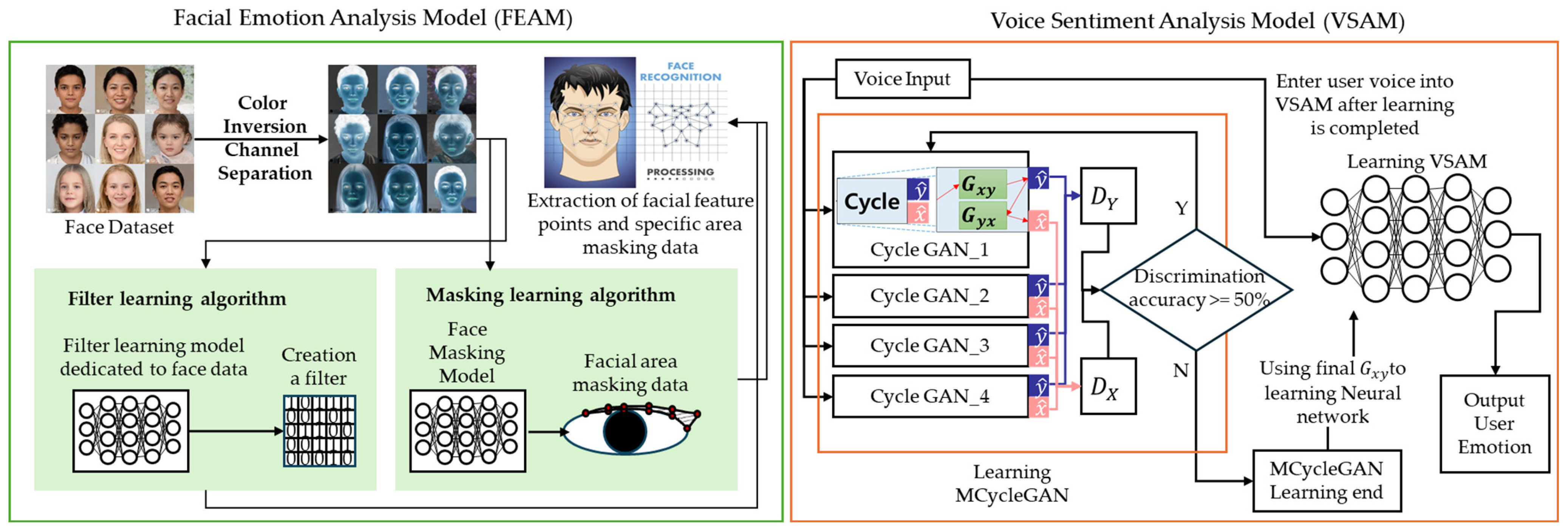
3. Design of the EAS

Figure 1 shows the structure of the FEAM and the VSAM used in EAS. The Face and Voice Recognition-based Emotion Analysis System (EAS) is composed of three primary modules: the Facial Emotion Recognition Module, the Voice Emotion Recognition Module, and the User Emotion Analysis Module. The system functions by first analyzing facial expressions using the facial features, followed by analyzing the tone, speech duration, and sentence structure of the voice to detect emotions. Finally, it integrates the emotions detected from both facial expressions and voice to provide a comprehensive analysis of the user’s overall emotional state.

Figure 1. The operation process of the facial expression-based emotion recognition and voice-based emotion recognition models used in EAS.

The Facial Emotion Recognition Module is subdivided into the Facial Feature Recognition Submodule and the Expression Recognition Submodule. The Facial Feature Recognition Submodule classifies the facial features (such as eyes, nose, mouth, ears, etc.) and infers the emotional state for each feature. The Expression Recognition Submodule then estimates the user’s facial emotions by combining the emotional states inferred from each feature with the overall facial expression.

The Voice Emotion Recognition Module first separates the user’s voice into tone and text components. It analyzes the emotions conveyed in the tone and then infers the emotional state from the content of the speech (text). By integrating the results from these modules, the EAS can provide a holistic evaluation of the user’s emotional state.

3.1. Constructing an Emotion Recognition Model Through Facial Expressions

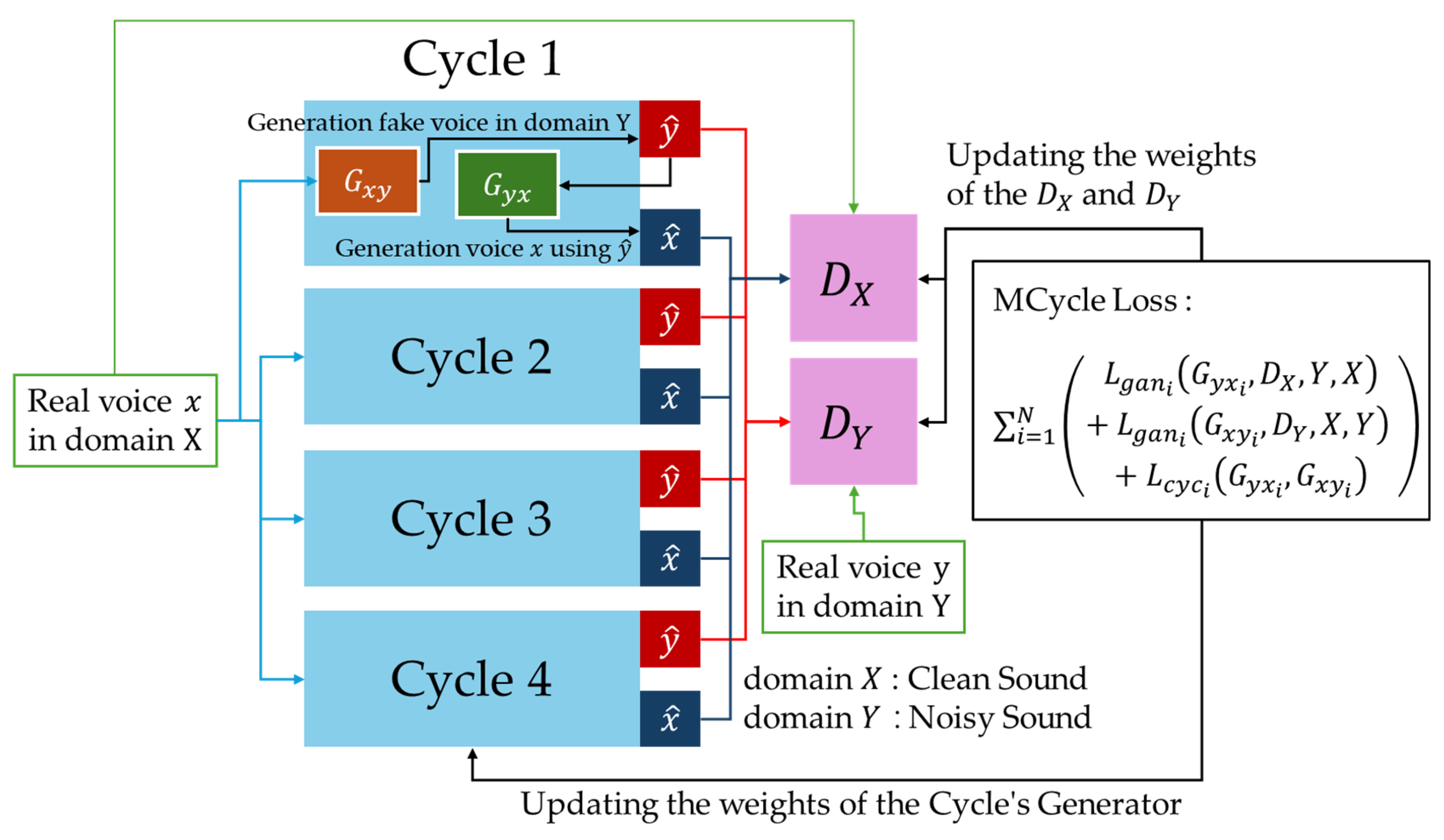
FEAM (Facial Expression Analysis Model) is a deep learning model designed to classify human facial expressions using 68 landmark coordinates as input. The model receives 68 landmark points as input data and classifies facial expressions into seven categories through hidden layers composed of fully connected neural networks. The data used for FEAM is based on facial images matched with seven emotions [22]. Although the dataset provides labeled video data in JSON format, the FEAM dataset was constructed by extracting 68 landmark points from the original image data and re-matching them with the labeled emotions. To achieve this, 68 landmarks were generated for each image using Dlib, a C++-based library, and OpenCV2. The coordinates of each landmark were then extracted and stored.

In this study, instead of the CNN models commonly used for facial expression recognition, a fully connected neural network is employed. Four models with different configurations are designed for the fully connected neural network utilized in FEAM, and the model that achieves the optimal results is selected for use in FEAM.

For optimal analysis, four different models of FEAM were designed with varying depths of hidden layers, as illustrated in Figure 2. Model A has four hidden layers with 32, 64, 64, and 32 nodes, respectively. Model B consists of six hidden layers with 32, 64, 128, 128, 64, and 32 nodes. Model C includes eight hidden layers with 32, 32, 64, 64, 128, 128, 64, and 32 nodes. Lastly, Model D has ten hidden layers with 32, 64, 64, 128, 256, 256, 128, 64, 32, and 32 nodes. Each layer uses ReLU as the activation function. The final layer is a softmax layer with seven nodes, corresponding to the number of output labels. The reason for using softmax is that when combined with Cross Entropy Error (CEE) in classification tasks, differentiating softmax with CEE allows for rapid computation of gradient values. Since the last softmax layer exists to enhance the differentiation speed of CEE during the training process, it is not used when deploying the model after training is complete.

Figure 2. The neural network models A, B, C, and D configured for the FEAM.

This paper also aims to compare the CNN models frequently used in emotion recognition with the fully connected neural network model employed in FEAM. The CNN-based model used for comparison is composed of three layers that perform convolution and one fully connected layer. Each layer uses ReLU as the activation function, and the convolution operations are performed with filters of size 3 × 3, moving the stride by 1 each time. The fully connected FC4 layer reshapes the 3D output from C3 into 1D, as it cannot process 3D data directly, and then outputs it using the ReLU activation function. The final FC5 layer has seven nodes with a softmax activation function to classify the output into seven facial expressions. Like the FEAM models, the FC5 layer is only used during training to enhance the processing speed of CEE and is not used during actual prediction.

3.2. MCycle GAN

MCycle GAN is designed to enhance the discriminator’s ability by training multiple cycles of the traditional Cycle GAN and ultimately selecting the generator from the cycle with the best performance. When removing noise from a noisy voice, a Cycle GAN-based model is used because it preserves the form of the original data, helping to maintain the structure of the original voice. Additionally, Cycle GAN can utilize unpaired training data between domains, which allows the collection of Clean Sound and Noisy Sound data separately for AI training.

In this paper, the domain Clean Sound is defined as $X$, and Noisy Sound is defined as $Y$. Data belonging to $X$ are referred to as $x$, and data belonging to $Y$ are referred to as $y$. The generator that converts $x$ to $y$ is called $G_{xy}$, and its inverse is $G_{yx}$. $D_{domain}$ refers to the discriminator (D), which determines whether the input data are real or fake data generated by the generator for that specific domain. MCycle GAN integrates two loss functions for backpropagation: Adversarial Loss and Cycle Consistency Loss. Adversarial Loss is one of the loss functions used in GANs, where the generator tries to better fool the discriminator, and the discriminator improves its ability to distinguish.

In this paper, when using a Cross Entropy Error (CEE)-based loss function for Adversarial Loss, there is a significant risk of encountering the Gradient Vanishing problem. Therefore, the LSGAN, an SSE (Sum of Squares of Error)-based loss function, is employed [16].

Adversarial Loss:

$$L_{gan}\left(G_{xy},{ D}_y, X, Y\right)=E_{y~P_{data}\left(Y\right)}\left[{\left(D_y\left(y\right)-1\right)}^2\right]+E_{x~P_{data}\left(x\right)}\left[D_y\right(G_{xy}{\left(x\right)}^2\left)\right]$$

Cycle Consistency Loss is a loss function that aims to make the generator’s output $G_{yx}\left(G_{xy}\left(X\right)\right)\approx X, G_{xy}\left(G_{yx}\left(Y\right)\right)\approx Y$. This ensures that the transformed data can be easily restored to its original form during training [14].

Cycle Consistency Loss:

$$L_{cyc}\left(G_{xy}, G_{yx}\right)=E_{x~P_{data}\left(x\right)}\left[\left|\left|G_{yx}\left(G_{xy}\left(x\right)\right)-x\right|\right|\right]+\left[\left|\left|G_{xy}\left(G_{yx}\left(y\right)\right)-y\right|\right|\right]$$

MCycle GAN uses an MCycle Loss, which integrates the two loss functions mentioned above. Since MCycle GAN consists of multiple cycles, there are multiple $L_{gan}$ and $L_{cyc}$. At this point, the generators for a particular cycle $G_{xy}$ and $G_{yx}$, are defined as $G_{x{y}_i}$ and $G_{y{x}_i}$, respectively, and the loss functions $L_{gan}$ and $L_{cyc}$ are defined as ${L_{gan}}_i$ and $L_{cy{c}_i}$, respectively. The formula for MCycle Loss is as follows:

MCycle Loss:

$$\begin{gathered} L_{mcyc}(L_{ga{n}_1}\left(G_{y{x}_1}, D_X, Y, X\right), L_{ga{n}_1}\left(G_{{xy}_1}, D_Y, X, Y\right),L_{cy{c}_1}\left(G_{y{x}_1}, G_{{xy}_1}\right),\dots , \\ {L}_{ga{n}_N}\left(G_{y{x}_N}, D_X, Y, X\right), L_{ga{n}_N}\left(G_{{xy}_N}, D_Y, X, Y\right), L_{cy{c}_N}\left(G_{y{x}_N}, G_{{xy}_N}\right)) \\ =\sum _{i=1}^N(L_{ga{n}_i}\left(G_{y{x}_i}, D_X, Y, X\right)+L_{ga{n}_i}\left(G_{{xy}_i}, D_Y, X, Y\right)+L_{cy{c}_i}\left(G_{y{x}_i}, G_{{xy}_i}\right)) \end{gathered}$$

$L_{mcyc}$ is a loss function that combines $L_{gan}$ and $L_{cyc}$ across all cycles of MCycle GAN in accordance with the multi-cycle structure. This allows simultaneous learning across multiple cycles while enhancing the training of the discriminator. Additionally, it offers the benefit of reusing a single discriminator for multiple generator models. Since multiple cycles are trained, by examining the output results of the generators, the generator that produces the highest-quality output can be selected and used.

3.3. Detailed Structure of the MCycle GAN

A cycle takes data from the Clean Sound domain x as input and produces two output data types:

Output 1: $G_{xy}\left(x\right)=\widehat{y}$

Output 2: $G_{yx}\left(\widehat{y}\right)=\widehat{x}$

Here, $\widehat{x}$ and $\widehat{y}$ refer to Fake Domain X data and Fake Domain Y data generated by the generators, respectively. Output 1, $\widehat{y}$, are the Fake Domain Y data generated by the generator $G_{xy}$ from an arbitrarily selected data point, $x$, in Domain X. Output 2, $\widehat{x}$, is the Fake Domain X data generated by the generator $G_{yx}$ from the output data, $\widehat{y}$, of Output 1.

MCycle GAN has a structure that uses multiple cycles, as shown in Figure 3. Multiple cycles receive arbitrary Domain X data, $x$, as input in parallel. Among the outputs of each cycle, the Fake Domain Y data, $\widehat{y}$, are used as the input to the discriminator, $D_y$, and the Fake Domain X data, $\widehat{x}$, are used as the input to the discriminator, $D_x$. $D_y$ receives either the Fake data, $\widehat{y}$, or the Real data, $y$, as input and outputs of the probability that the data are real. Similarly, $D_x$ receives $\widehat{x}$ and $x$ as inputs and outputs of the probability that the input data are real.

Figure 3. Architecture of MCycle GAN(4).

During training, the weights of the generators in each cycle, as well as the discriminators $D_x$ and $D_y$, are updated according to the MCycle Loss. When the discrimination accuracy of $D_x$ and $D_y$ reaches 50%, the training is complete. Ultimately, the cycle that best fools the discriminator is considered the most effective, and that cycle is selected for use.

In this paper, $G_{xy}$, one of the components of the cycle, is the generator that takes clean sound data as input and generates noisy sound data, while $G_{yx}$ is its inverse. Therefore, to generate sound data with the noise removed, $G_{yx}$ is used as the final noise reduction model.

The generator of MCycle GAN uses a ResNet-based CNN model to preserve the details of the input data and prevent bottlenecks in the data [17]. The generator is trained in the direction of reducing the Adversarial Loss. A smaller Adversarial Loss indicates that the generator is better at fooling the discriminator.

The discriminator uses a CNN-based image classification model with Leaky ReLU as the activation function. The discriminator trained with Leaky ReLU can pass stronger gradients to the generator compared to ReLU [18].

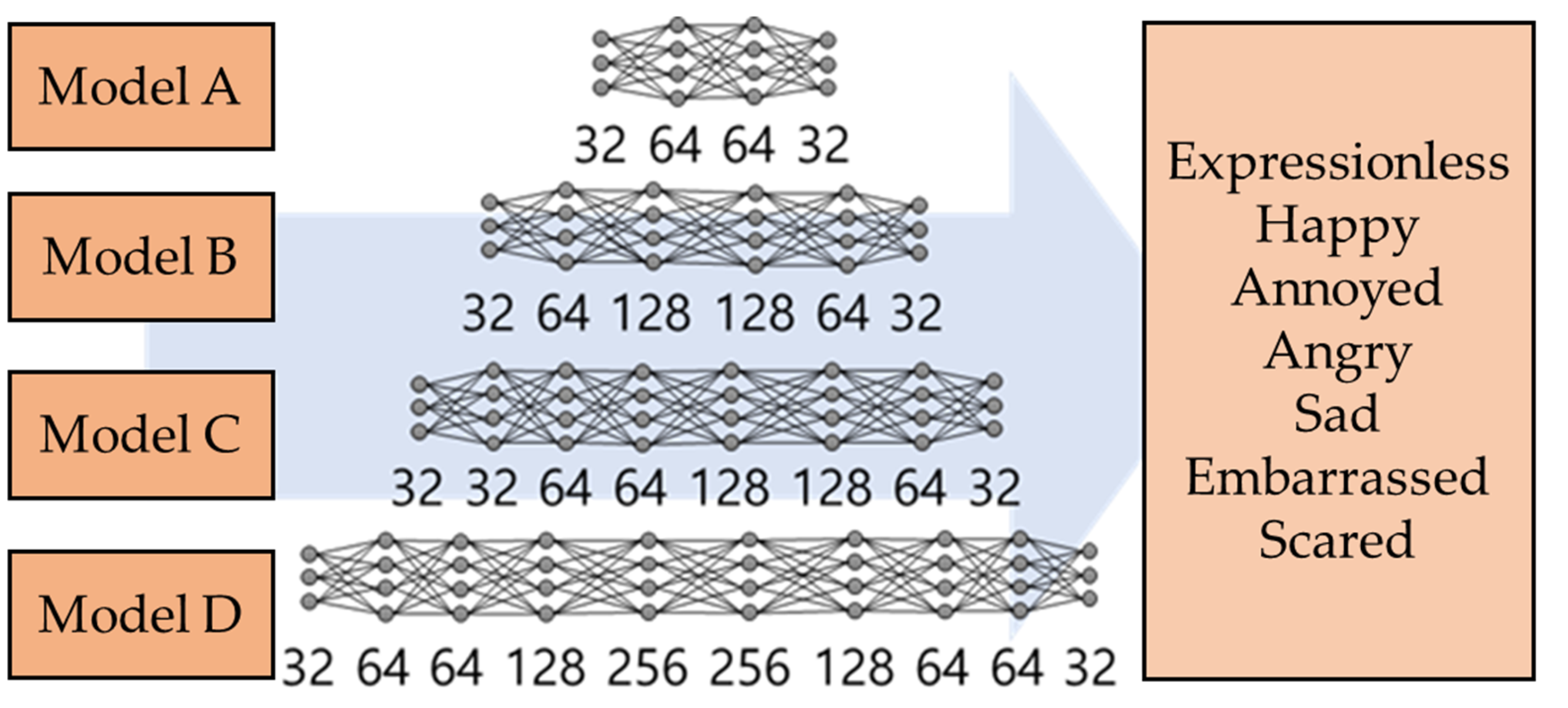
3.4. Constructing an Metaverse Emotion Recognition Model

The Metaverse Emotion Recognition Model (MERM) is designed to integrate emotional states detected by both the Voice Sentiment Analysis Model (VSAM) and the Facial Emotion Analysis Model (FEAM). Specifically, MERM considers only matching emotion values from VSAM and FEAM to ensure that the final emotional output is accurate and aligns with the user’s authentic state.

In this process, both VSAM and FEAM independently analyze emotional states, outputting seven primary emotion values: happiness, sadness, anger, fear, surprise, disgust, and neutrality. Each emotion from VSAM is paired with the corresponding emotion from FEAM. Only when the emotion values for a specific category (e.g., happiness or sadness) are similar or consistent across both models are they merged into a single value.

This selective merging method minimizes conflicting emotional readings and enhances the reliability of the detected emotional state within the metaverse, ultimately ensuring that virtual entities can react to user emotions in a realistic and synchronized manner. Figure 4 shows the neural network configuration of MERM.

Figure 4. The architecture of MERM.

4. Simulation

4.1. Simulation of the FEAM

To construct a model for facial expression classification, a training dataset must be collected. The data utilize facial video data that display expressions. The collected facial video data are classified into seven expressions—neutral, anger, anxiety, hurt, sadness, happiness, and embarrassment—provided by AI-Hub’s Composite Videos for Korean Emotion Recognition [22].

For a comparison between the proposed DFLM and traditional CNN-based models in this study, the collected data and labels cannot be used as-is. Traditional CNN models input two-dimensional color data corresponding to the width and height of the image, whereas DFLM uses facial landmarks and, thus, requires 68 coordinate values as input.

To prepare the data for training, facial regions are detected in the video frames containing the seven types of emotional expressions. Based on the detected facial regions, landmarks are extracted to create data consisting of 68 coordinate values. These 68 coordinate values are then utilized as training data for DFLM.

For CNN models, the facial regions are cropped from the raw data and resized to 256 × 256 pixels. The original RGB color images are converted to grayscale to generate 256 × 256 grayscale images. A total of 7000 facial images are used, with 1000 images for each expression. Of these, 70% are used as training data, and the remaining 30% are used as validation data to verify the accuracy of the training process.

Accuracy is a simple method for measuring performance, calculated as the ratio of the number of correctly predicted data points to the total number of data points. Specifically, it refers to the ratio of correct predictions to the total number of cases, which includes both correctly and incorrectly predicted outcomes.

Figure 5 shows the training and validation accuracy for FEAM models A, B, C, and D across epochs during the training process. As depicted in Figure 5, as training progresses, a gap emerges between the training accuracy and validation accuracy of the models. While the training accuracy continues to increase, the validation accuracy grows at a slower rate, indicating that this gap is a sign of overfitting. Overfitting refers to the model excessively fitting the training data, leading to a decline in generalization performance on new, unseen data.

Figure 5. The training and validation accuracy for FEAM models A–D across epochs during the training process.

Since the training data are a subset of the actual data, the error decreases for the training data, but the error tends to increase for the actual data. In Figure 5, looking at each model A, B, C, and D, the difference between training accuracy and validation accuracy decreases as it moves toward model D. Through the experiment, it was found that having more layers is advantageous in reducing overfitting.

Figure 6 is a graph comparing the accuracy of each model using test data after 500 iterations of training. The accuracy of each model tested with the test data shows that model A has an accuracy of 0.4757, model B has 0.4438, model C has 0.5171, and model D has 0.5305, indicating that model D has the highest recognition rate. According to this metric, it can be observed that as the depth of the layers increases, the accuracy of learning tends to improve.

Figure 6. A graph comparing the accuracy of each model using test data after 500 iterations of training.

In the model trained with CNN as shown in Figure 7, the accuracy was 0.5307, which is similar to the value of DFLM. However, it is evident that the gap between the training data and validation data continued to widen, indicating that the model stopped learning effectively. Due to the nature of CNN models, when the sample size of the training data is small, overfitting issues arise. The widening gap between training accuracy and validation accuracy indicates that overfitting occurred during training with the CNN model.

Figure 7. Accuracy of existing CNN models confirmed with test data.

In the experimental setup of this study, the gap between training accuracy and validation accuracy began to widen from epoch 3. Around the point where an accuracy of approximately 0.45 was achieved, the difference between training and validation accuracy started to increase. After 25 epochs, while training accuracy reached up to 0.9, validation accuracy plateaued around 0.5 and did not improve further.

$$\begin{gathered} F_1=2\ast {\displaystyle \frac{1}{\frac{1}{r}+\frac{1}{p}}}={\displaystyle \frac{p\ast r}{p+r}} \\ \mathrm{p}=\mathrm{precision}, \mathrm{r}=\mathrm{recall} \end{gathered}$$

Accuracy can be misleading statistics depending on the data. For instance, in a medical AI system designed to diagnose cancer, a model that always predicts a negative result would achieve a high accuracy because there are significantly more healthy individuals than those with cancer. Such a model, despite having high accuracy, is essentially meaningless. In this context, recall (also known as sensitivity) becomes a useful metric. Recall measures the proportion of actual positive cases that are correctly identified as positive. For example, if there are 10 positive cases and the model predicts all as negative, the recall will be 0 (0/10), indicating a problem with the model.

Precision, on the other hand, contrasts with recall. If a model always predicts positive, the recall will be 1, as all actual positive cases are identified. However, this model would be as ineffective as one predicting all negatives if it produces many false positives. Precision addresses this issue by measuring the proportion of true positives among all instances the model predicted as positive. For example, if there are 10 positive cases and the model predicts 100 instances as positive, with only 10 being true positives, the precision would be 0.1 (10/100), indicating a problem with the model.

In this paper, we use the F1 score, a combined statistic of precision and recall. The F1 score is the harmonic mean of precision and recall. The reason for using the harmonic mean is that it ensures that the F1 score is low when either precision or recall is close to zero.

Figure 8 shows the F1 scores for each model. Model A has an F1 score of 0.4189, Model B has 0.3774, Model C has 0.4562, and Model D has 0.4752. It can be observed that the F1 score tends to increase from Model A to Model D, with Model D demonstrating the best performance.

Figure 8. The F1 scores for each model.

In artificial intelligence, the time required for model training, and the time it takes for the trained model to make predictions are critical metrics. When comparing the training times, DFLM takes approximately 1 s per epoch, while the CNN model requires about 100 s. Furthermore, for testing, the CNN model needs 8.128 s per step, whereas DFLM completes the evaluation of test data in just 0.004 s per step. This indicates that the proposed model operates at a very fast speed when put into practical use. The number of samples used for training was insufficient, which resulted in a low overall accuracy and a large variance in accuracy during training. This needs to be improved. We expect that future research will increase the training data and explore the use of various deep learning models, rather than just fully connected neural networks, to improve accuracy.

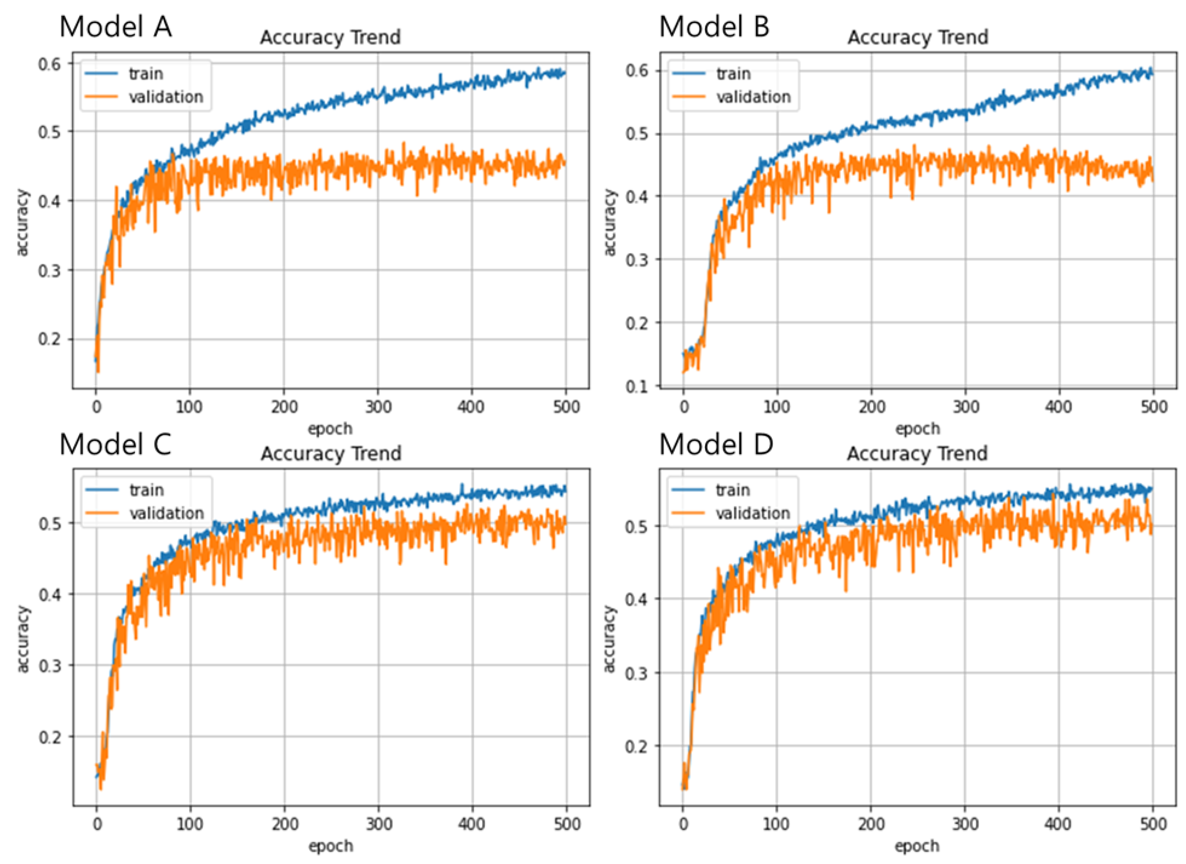
4.2. Simulation of the MERM

For the dataset used in training, 500 speech data samples for emotion analysis were referenced from AI-Hub [23], and 2000 environmental sound samples (.wav) were referenced from ESC-50: Dataset for Environmental Sound Classification [24]. Speech data for emotion analysis and environmental sound data were randomly extracted and synthesized to generate 2000 noisy sound samples (.wav). Since the generator and discriminator are CNN-based models designed for image processing in deep learning, the audio data were converted into spectrograms (.png, 196 × 128) and used as images. The performance evaluation of MERM is conducted using three metrics: error compared to the original data, training time, and the discriminator’s loss function.

• Error Compared to the Original Data: This metric is calculated by inputting 10 samples of data generated by the generator, which incorporates noise into the original data, and predicting the data. The evaluation measures the sum of squared differences between the predicted data and the original data. A lower value indicates that the model outputs data more like the original data.
• Training Time: This metric represents the time required for the model to complete training for 40 epochs. A shorter training time indicates a faster model.
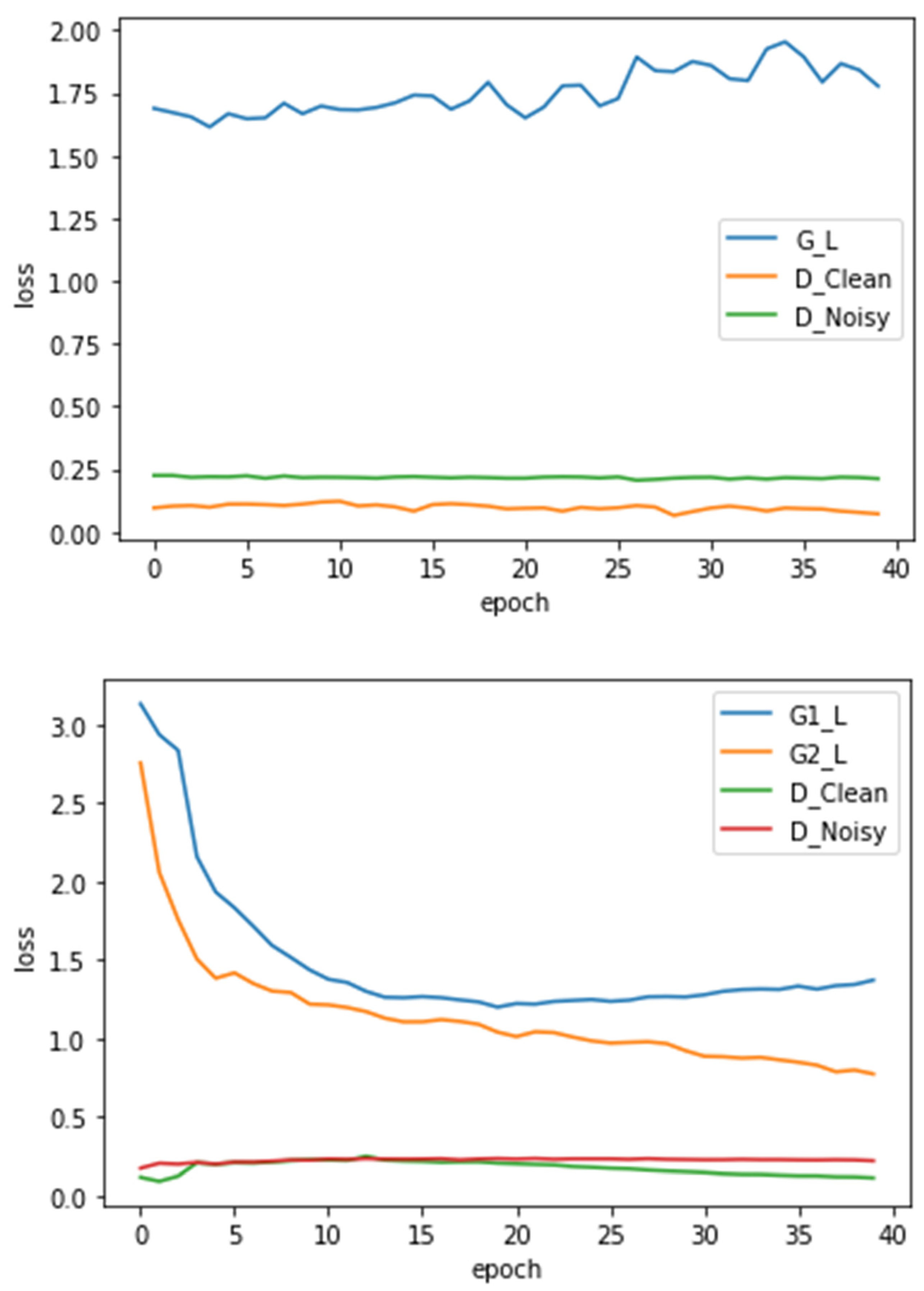
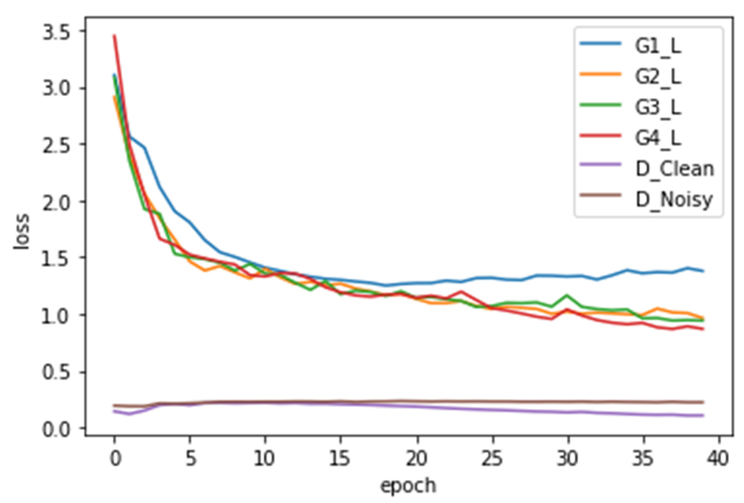
• Discriminator’s Loss Function: This value reflects the discriminator’s ability to detect the generator’s forgery. A lower value indicates that the discriminator effectively identifies forged data. Conversely, a higher value suggests that the generator is more successful at deceiving the discriminator or that the discriminator has been enhanced. The evaluation involves using the generator to predict 50 test samples and calculating the discriminator’s loss function value.

Table 1 presents the evaluation of noise reduction performance for each model, where MCycleGAN(2) exhibits the lowest error of 14.781. This indicates that MCycleGAN(2) effectively handles noise while maintaining similarity to the original data compared to other models. In terms of training time, CycleGAN has the shortest duration at 2037 s, whereas MCycleGAN has the longest at 7590 s. The longer training time for MCycleGAN is attributed to its use of multiple cycles, making it relatively slower than other models.

Table 1. The evaluation of noise reduction performance for each model.

	Cycle GAN	MCycle GAN(2)	MCycle GAN(4)
Error	17,150	14,781	15,312
Training time (s)	2037	3838	7590
Discriminator loss function	11.2139	0.2813	0.2409

Regarding the discriminator’s loss function, CycleGAN has a relatively high value of 11.2139 compared to other models. In contrast, MCycleGAN shows minimal differences based on the number of cycles: 0.2813 for two cycles and 0.2409 for four cycles. This suggests that CycleGAN’s generator does not adequately deceive the discriminator. When comparing MCycleGAN with two cycles versus four cycles, it is observed that four cycles require approximately twice as much training time as two cycles, though the performance improvement is marginal. Consequently, the model with two cycles is deemed to offer better training time efficiency compared to the model with four cycles.

Figure 9 show the loss of the generator and the loss of the discriminator during the training of each model over 40 epochs. During the same epoch, it can be observed that the MCycle GAN model moves in a direction where the generator’s loss function decreases. While at epoch 0 it performs worse compared to Cycle GAN, from epoch 5 onward, it shows better performance than Cycle GAN. However, in the case of Cycle GAN, it was observed that the generator’s loss function tends to increase during training. Therefore, it is predicted that more epochs may be needed for Cycle GAN.

Figure 9. The loss of the generator and the loss of the discriminator during the training of each model over 40 epochs.

As for the loss function of the discriminator, at the 40th epoch, $D_{clean}$ shows the following values: MCycle GAN(4) = 0.1051, MCycle GAN(2) = 0.1100, Cycle GAN = 0.0714, indicating that the discriminator of MCycle GAN makes more errors. Although Cycle GAN’s $D_{clean}$ is smaller, the larger $G_L$ suggests that the generator is not yet proficient in creating realistic fake data.

5. Conclusions

From the moment VR and AR avatars became deeply integrated into our society, the issue of how virtual objects in these environments react like real people has become increasingly significant. Contemporary AI no longer focuses solely on problem-solving but has also made notable advancements in areas such as music, art, and conversation. Therefore, for virtual objects in the metaverse to interact more naturally with real-world entities, precise emotional analysis is essential, whether it is to accurately represent user emotions using VR or AR avatars or to express AI emotions through avatars.

This paper proposes an Emotion Analysis System (EAS) for accurate emotion analysis, which simultaneously recognizes the user’s voice and facial expressions. EAS uses a microphone and camera to analyze the user’s voice and facial expressions and then processes the results through a neural network to determine the user’s emotions accurately. EAS consists of three modules:

• Facial Emotion Analysis Model (FEAM): This model receives facial expressions as input and classifies them into seven emotions using facial landmarks.
• Voice Sentiment Analysis Model (VSAM): This model extracts voices from noisy environments using McycleGAN to accurately identify emotions from the user’s voice.
• Comprehensive Sentiment Analysis Module (CSAM): This module receives the results from FEAM and VSAM and accurately analyzes the current emotions of the user.

To validate the proposed system, two experiments were conducted. The first experiment tested the effectiveness of FEAM. It was observed that models with fewer layers quickly overfit. Simulation results showed that FEAM achieved an accuracy of 0.51 and an F1 score of A, while the CNN model achieved an accuracy of 0.5307 and an F1 score of A. FEAM completed the evaluation of test data in just 0.004 s per step, whereas the CNN model required 8.128 s per step. This indicates that reducing the input data and lightweighting the model can lead to faster processing.

The second experiment tested the effectiveness of MCycleGAN. In noise handling, MCycleGAN showed lower error rates and lower discriminator loss functions compared to GAN and CycleGAN. This indicates that MCycleGAN maintains the original voice shape while handling noise and that the processed data are not significantly different from the Clean Baby Sound domain, effectively deceiving the discriminator.

However, the current EAS only analyzes user emotions and does not implement emotion-based expressions. Additionally, research into the application of analyzed emotions and related fields has not been conducted. Future research should focus on developing AI models that can generate appropriate facial expressions or voices based on emotions or explore applications of the analyzed emotions.

References

1. Bae, J.H.; Wang, B.H.; Lim, J.S. Study for Classification of Facial Expression using Distance Features of Facial Landmarks. J. IKEEE 2021, 25, 613–618. [Google Scholar]
2. An, Y.-E.; Lee, J.-M.; Kim, M.-G.; Pan, S.-B. Classification of Facial Expressions Using Landmark-based Ensemble Network. J. Digit. Contents Soc. 2022, 23, 117–122. [Google Scholar] [CrossRef]
3. Gu, J.; Kang, H.C. Facial Landmark Detection by Stacked Hourglass Network with Transposed Convolutional Layer. J. Korea Multimed. Soc. 2021, 24, 1020–1025. [Google Scholar]
4. Kim, D.Y.; Chang, J.Y. Integral Regression Network for Facial Landmark Detection. J. Broadcast Eng. 2019, 24, 564–572. [Google Scholar]
5. Sohn, M.-K.; Lee, S.-H.; Kim, H. Analysis and implementation of a deep learning system for face and its landmark detection on mobile applications. In Proceedings of the Symposium of the Korean Institute of Communications and Information Sciences, Seoul, Republic of Korea, 16–18 June 2021; pp. 920–921. [Google Scholar]
6. Yoon, K.-S.; Lee, S. Music player using emotion classification of facial expressions. In Proceedings of the Korean Society of Computer Information Conference; Korean Society of Computer Information: Seoul, Republic of Korea, 2019; Volume 27, pp. 243–246. [Google Scholar]
7. Choi, I.-K.; Song, H.; Lee, S.; Yoo, J. Facial Expression Classification Using Deep Convolutional Neural Network. J. Broadcast Eng. 2017, 22, 162–172. [Google Scholar]
8. Choi, W.; Kim, T.; Bae, H.; Kim, J. Comparison of Emotion Prediction Performance of CNN Architectures; Korean Institute of Information Scientists and Engineers: Daejeon, Republic of Korea, 2019; pp. 1029–1031. [Google Scholar]
9. Salimov, S.; Yoo, J.H. A Design of Small Scale Deep CNN Model for Facial Expression Recognition using the Low Resolution Image. J. Korea Inst. Electron. Commun. Sci. 2021, 16, 75–80. [Google Scholar]
10. Park, J.H. A Noise Filtering Scheme with Machine Learning for Audio Content Recognition. 2019.02. Available online: https://repository.hanyang.ac.kr/handle/20.500.11754/100017 (accessed on 9 January 2024).
11. Lee, H.-Y. A Study on a Non-Voice Section Detection Model among Speech Signals using CNN Algorithm. J. Converg. Inf. Technol. 2021, 11, 33–39. [Google Scholar]
12. Lim, K.-H. GAN with Dual Discriminator for Non-stationary Noise Cancellation. In Proceedings of the Symposium of the Korean Institute of Information Scientists and Engineers, Republic of Korea, 18 December 2019. [Google Scholar]
13. Pascual, S.; Serra, J.; Bonafonte, A. Time-domain Speech Enhancement Using Generative Adversarial Networks. Speech Commun. 2019, 114, 10–21. [Google Scholar] [CrossRef]
14. Michelsanti, D.; Tan, Z.H. Conditional generative adversarial networks for speech enhancement and noise-robust speaker verification. arXiv 2017, arXiv:1709.01703. [Google Scholar]
15. Zhu, J.Y.; Park, T.; Isola, P.; Efros, A.A. Unpaired image-to-image translation using cycle-consistent adversarial networks. In Proceedings of the IEEE International Conference on Computer Vision, Venice, Italy, 22–29 October 2017. [Google Scholar]
16. Lai, W.H.; Wang, S.L.; Xu, Z.Y. CycleGAN-Based Singing/Humming to Instrument Conversion Technique. Electronics 2022, 11, 1724. [Google Scholar] [CrossRef]
17. Mao, X.; Li, Q.; Xie, H.; Lau, R.Y.; Wang, Z.; Paul Smolley, S. Least squares generative adversarial networks. In Proceedings of the IEEE International Conference on Computer Vision, Venice, Italy, 22–29 October 2017. [Google Scholar]
18. He, K.; Zhang, X.; Ren, S.; Sun, J. Deep residual learning for image recognition. In Proceedings of the IEEE Conference on Computer Vision and Pattern Recognition, Las Vegas, NV, USA, 27–30 June 2016. [Google Scholar]
19. Radford, A.; Metz, L.; Chintala, S. Unsupervised representation learning with deep convolutional generative adversarial networks. arXiv 2015, arXiv:1511.06434. [Google Scholar]
20. Yamamoto, S.; Yoshitomi, Y.; Tabuse, M.; Kushida, K.; Asada, T. Recognition of a baby’s emotional cry towards robotics baby caregiver. Int. J. Adv. Robot. Syst. 2013, 10, 86. [Google Scholar] [CrossRef]
21. Hwang, I.-K.; Song, H.-B. AI-based Infant State Recognition Using Crying Sound. J. Korean Inst. Inf. Technol. 2019, 17, 13–21. [Google Scholar]
22. Composite Images for Korean Emotion Recognition. Available online: https://www.aihub.or.kr/aihubdata/data/view.do?currMenu=115&topMenu=100&aihubDataSe=realm&dataSetSn=82 (accessed on 2 April 2024).
23. Conversational Speech Dataset for Sentiment Classification. Available online: https://aihub.or.kr/aihubdata/data/view.do?currMenu=115&topMenu=100&dataSetSn=263 (accessed on 2 April 2024).
24. ESC-50: Dataset for Environmental Sound Classification, Noisy Sound Data Set. Available online: https://github.com/karolpiczak/ESC-50 (accessed on 2 April 2024).
Disclaimer/Publisher’s Note: The statements, opinions and data contained in all publications are solely those of the individual author(s) and contributor(s) and not of MDPI and/or the editor(s). MDPI and/or the editor(s) disclaim responsibility for any injury to people or property resulting from any ideas, methods, instructions or products referred to in the content.
Article Metrics
Citations
Article Access Statistics
Multiple requests from the same IP address are counted as one view.