

Development of a Reduced Order Model-Based Workflow for Integrating Computer-Aided Design Editors with Aerodynamics in a Virtual Reality Dashboard: Open Parametric Aircraft Model-1 Testcase


Abstract
1. Introduction
- Development of a fully automated workflow that connects CAD and mesh: The proposed approach is highly innovative, combining the benefits of mesh morphing and parametric CAD. The parameterization is defined at the CAD level, and the CAD modifications are encoded in a way that can be used to deform the mesh. This ensures excellent geometry control while minimizing computation times.
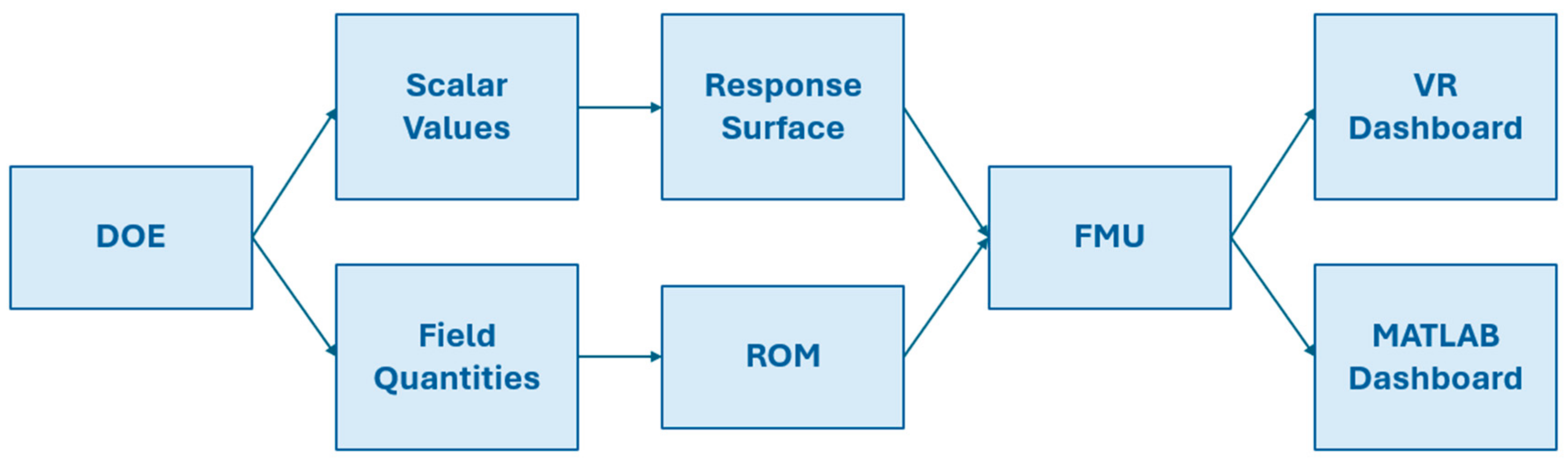
- Use of ROMs and FMUs: These techniques make CFD analysis results available in real time in any environment.
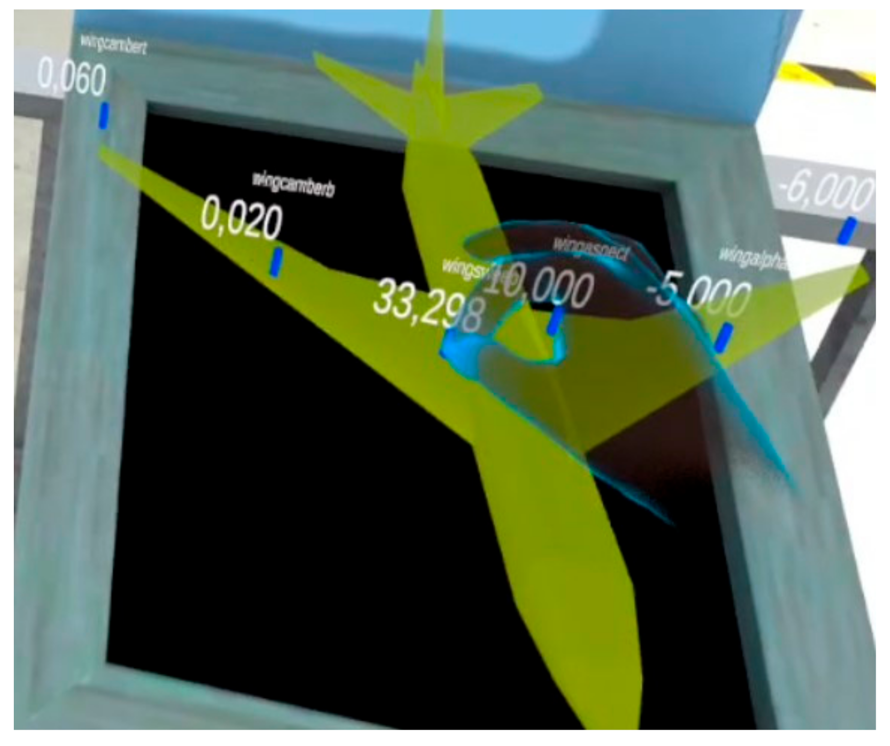
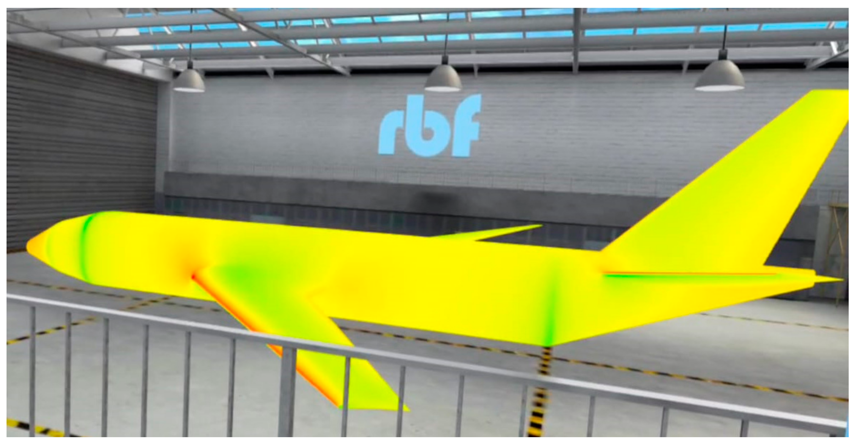
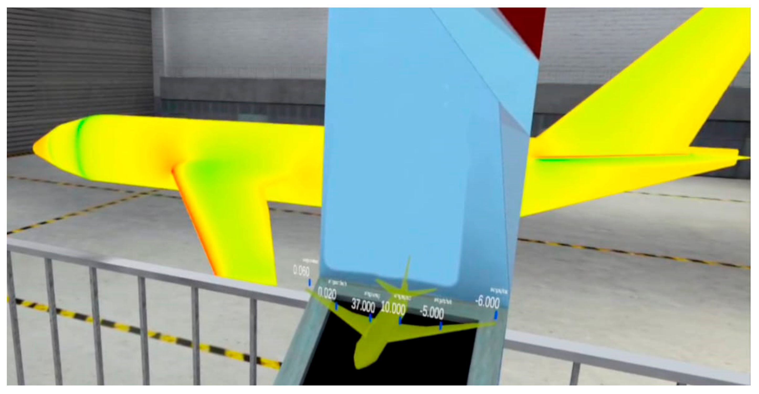
- Integration of VR: Virtual reality is employed to create an interactive dashboard where the user, using their hands or sliders, can adjust the geometry and visualize in real time how the aerodynamics change, both in terms of scalar values and field quantities.
- In this paragraph, a quick introduction is given on the state of the art for the topics addressed, and the structure of the paper is outlined;
- In Section 2, a theoretical background is provided, and the tools used are presented;
- In Section 3, the stage case and the OPAM project are presented;
- In Section 4, we focus on the method used, a hybrid workflow that exploits CAD-based parameterization and a mesh morphing technique;
- In Section 5, several dashboards are shown in which the results are deployed. In particular, the MATLAB and VR dashboards are shown;
- In Section 6, the testcase is shown.
2. Theoretical Background
2.1. Mesh Morphing and Radial Basis Functions (RBFs)
2.2. Design of Experiment and Response Surface
- G(x) is the aggregated response surface,
- Ri(x) are the individual response surfaces,
- wi are the optimized weights.
2.3. Reduced Order Models
- is a diagonal matrix composed of σi, the singular values of matrix .
- and are matrices such that = and = .
- are the learning solution vectors (learning snapshots i).
2.4. Functional Mock-Up Interface
- Model Exchange (ME): Allows the exchange of models described as systems of differential or algebraic equations. This type of FMU is integrated directly into the host simulator.
- Co-Simulation (CS): Includes an internal solver, enabling the FMU to run the simulation autonomously while communicating with other models or simulations through standardized interfaces.
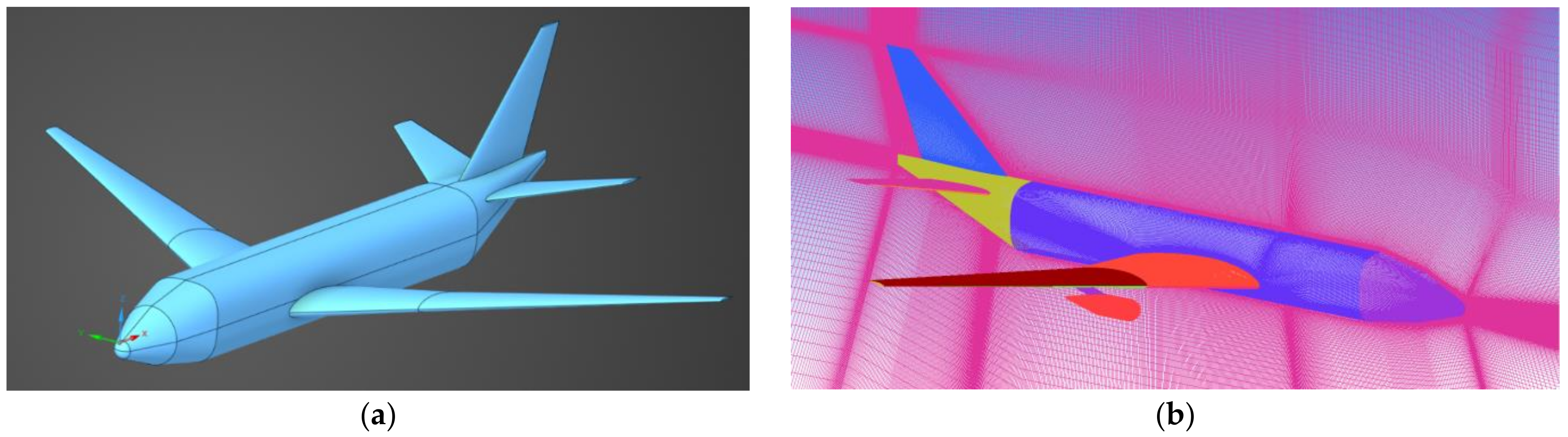
3. Reference Case
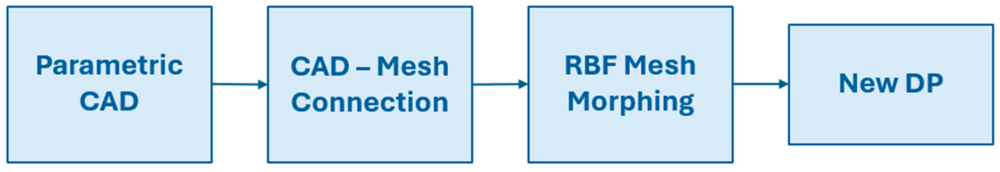
4. Hybrid Workflow
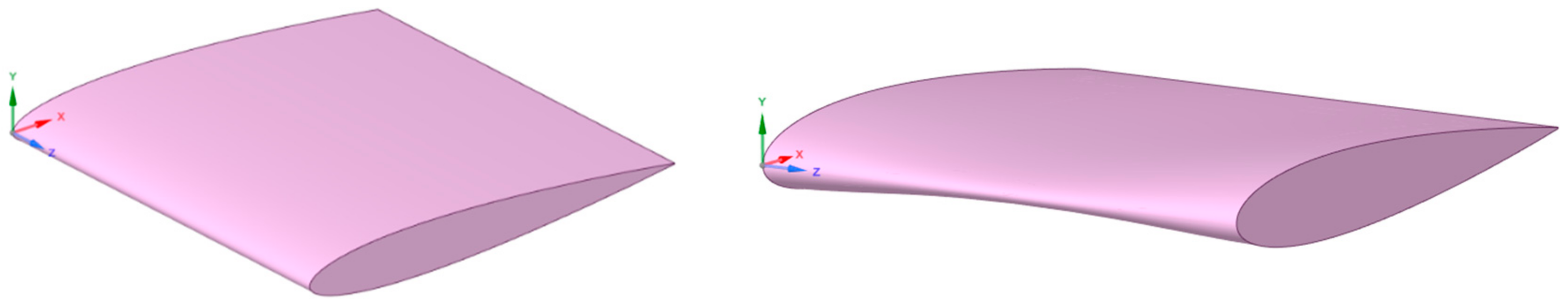
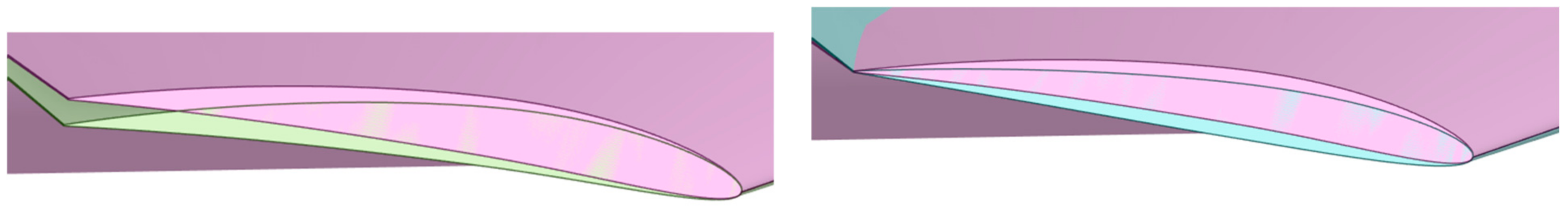
4.1. Parametric CAD
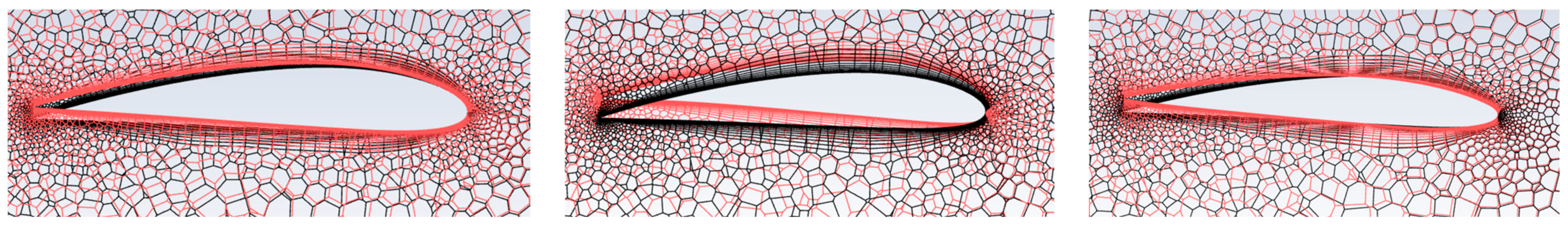
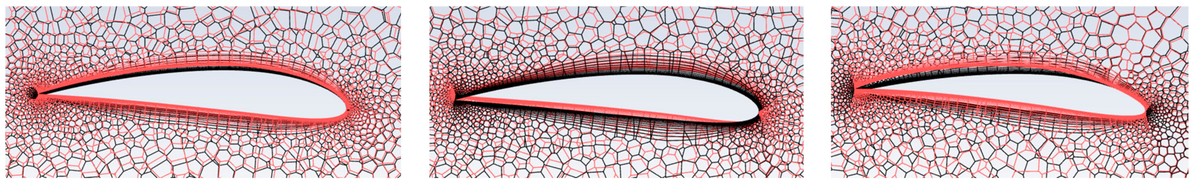
4.2. CAD–Mesh Connection
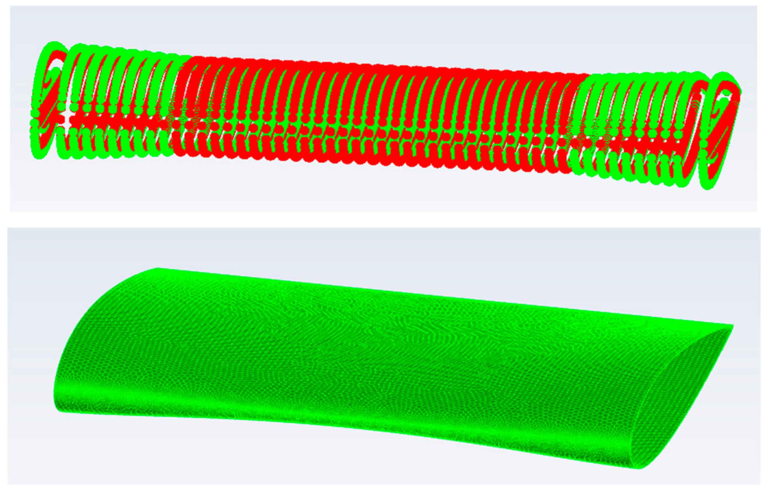
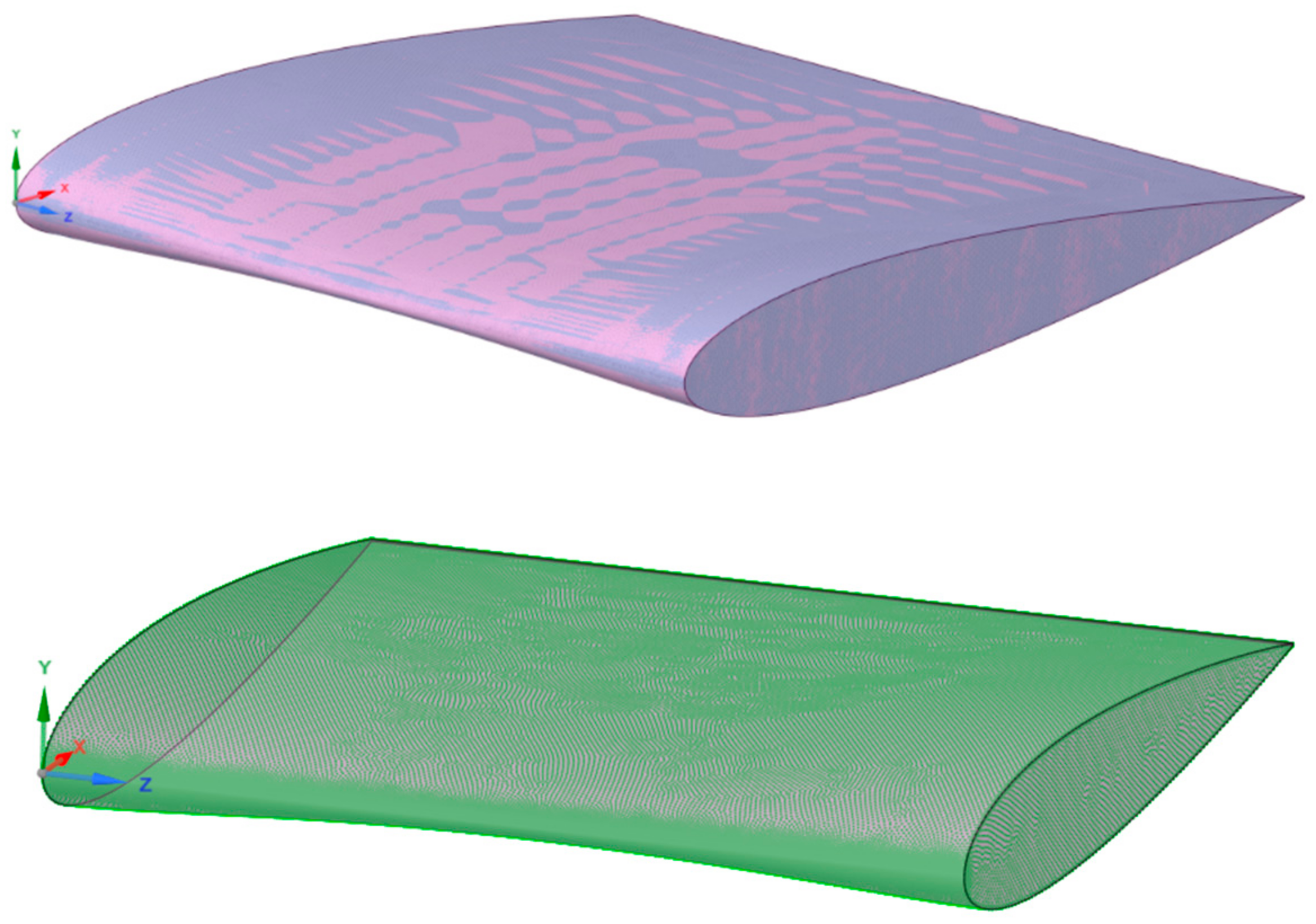
4.3. RBF Volume Mesh Morphing
5. Design Dashboard
- Create the dataset;
- Create a metamodel that provides the necessary information in real-time as the considered CAD-based parameters vary;
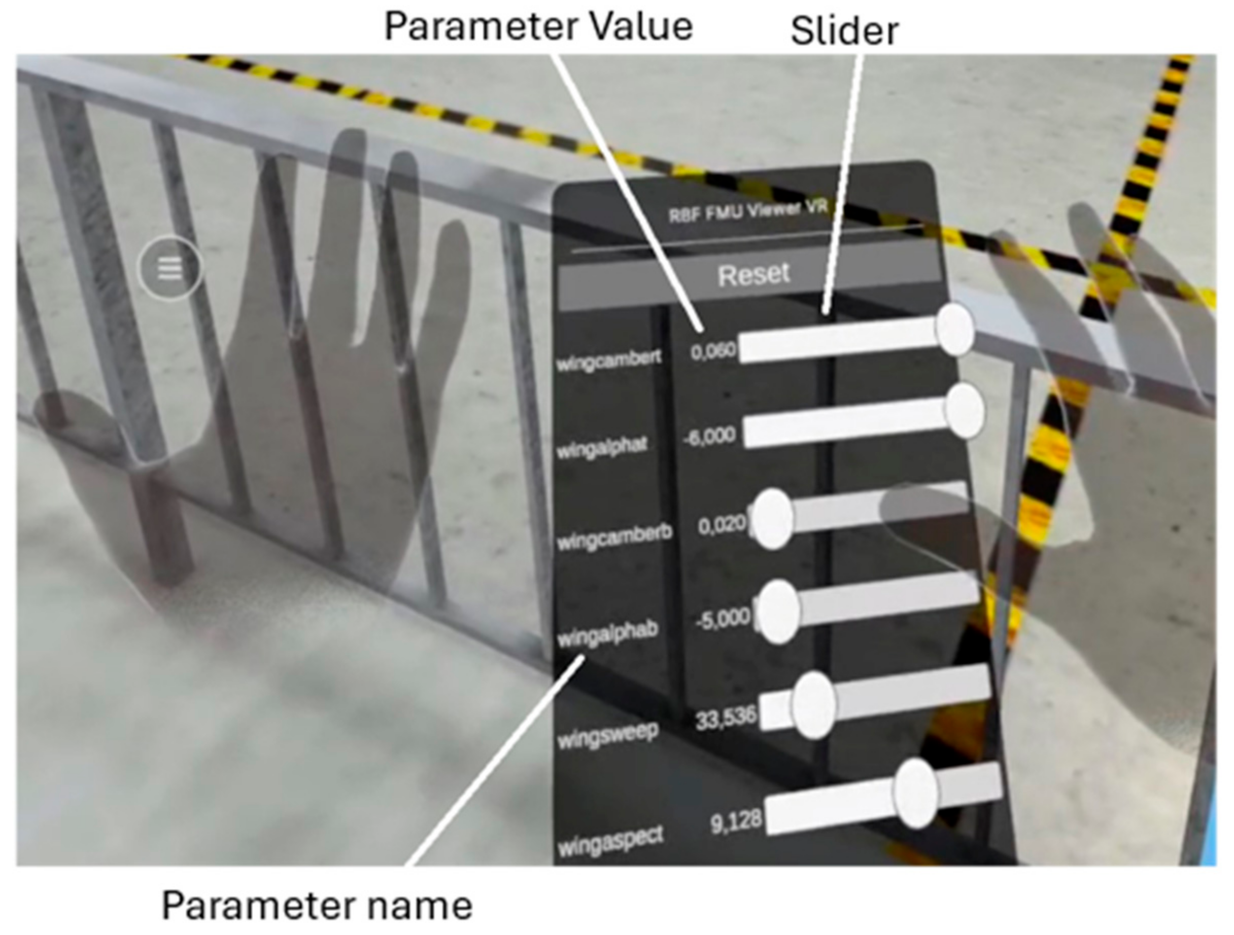
- Define interactive handles to be positioned in the 3D scene;
- Visualize everything in real-time on the MATLAB dashboard and on the Meta Quest 3 headset in VR;
- Enable real-time interaction with the model by creating sliders or handles.
- Global scalar quantities of interest (drag, lift, and efficiency);
- Coordinates x, y, and z of each surface node;
- CFD results at the x, y, and z coordinates (pressure values).
5.1. Matlab Dashboard
5.1.1. FMU Import
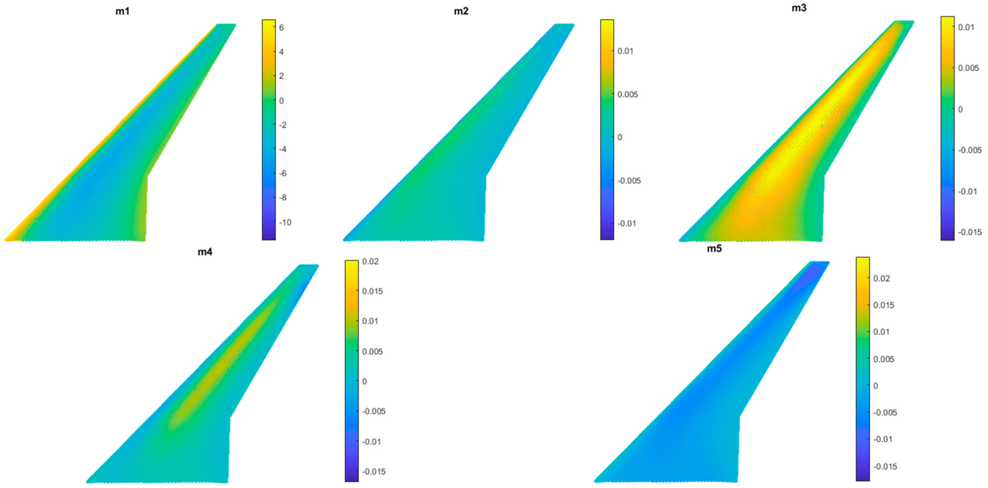
- One controls the generation of modes, which is executed only once, and the modes are stored as vectors.
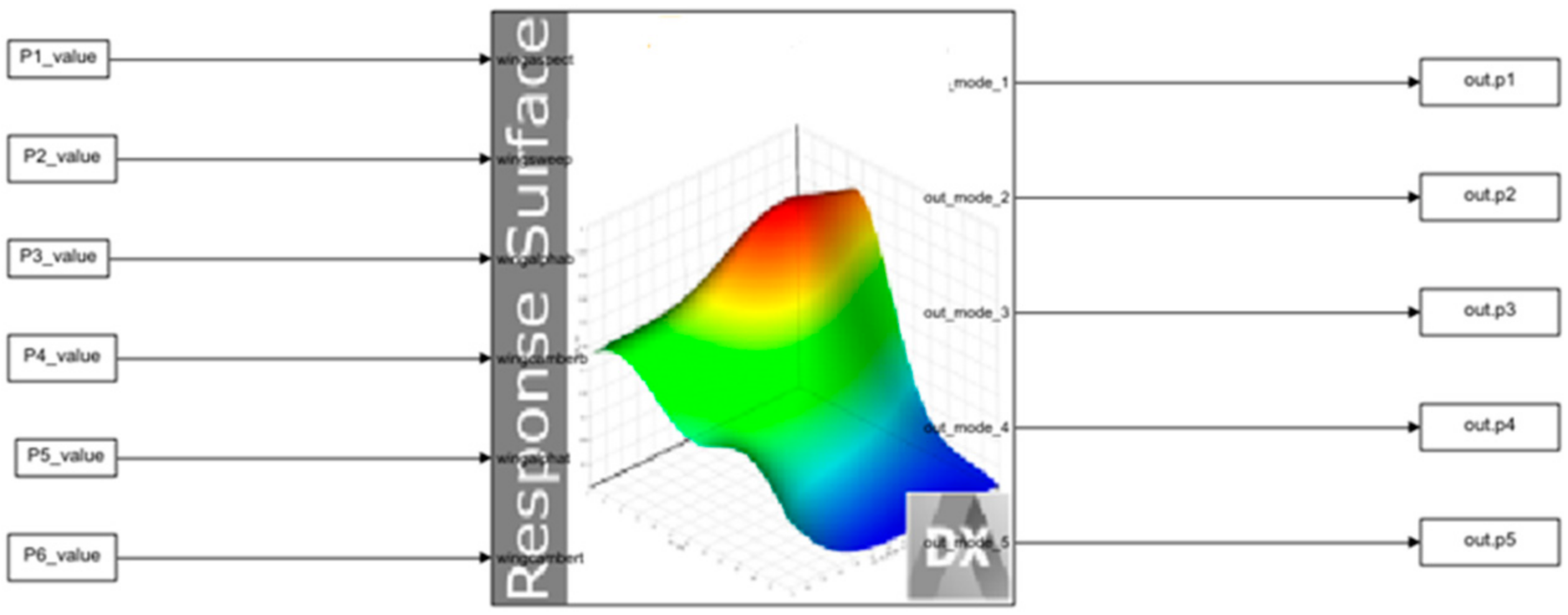
- The other controls the generation of weights, containing the RS that outputs the weights for each n-tuple of inputs (Figure 9).
5.1.2. Optimization Dashboard
5.2. VR Graphical Dashboard
5.2.1. Import Module
- Baseline 3D mesh (STL file)
- FMUs containing transformations from input parameters to mode coefficients
- Mode matrix of the mesh ROM (CSV file)
- Pressure ROM modes matrix (CSV file)
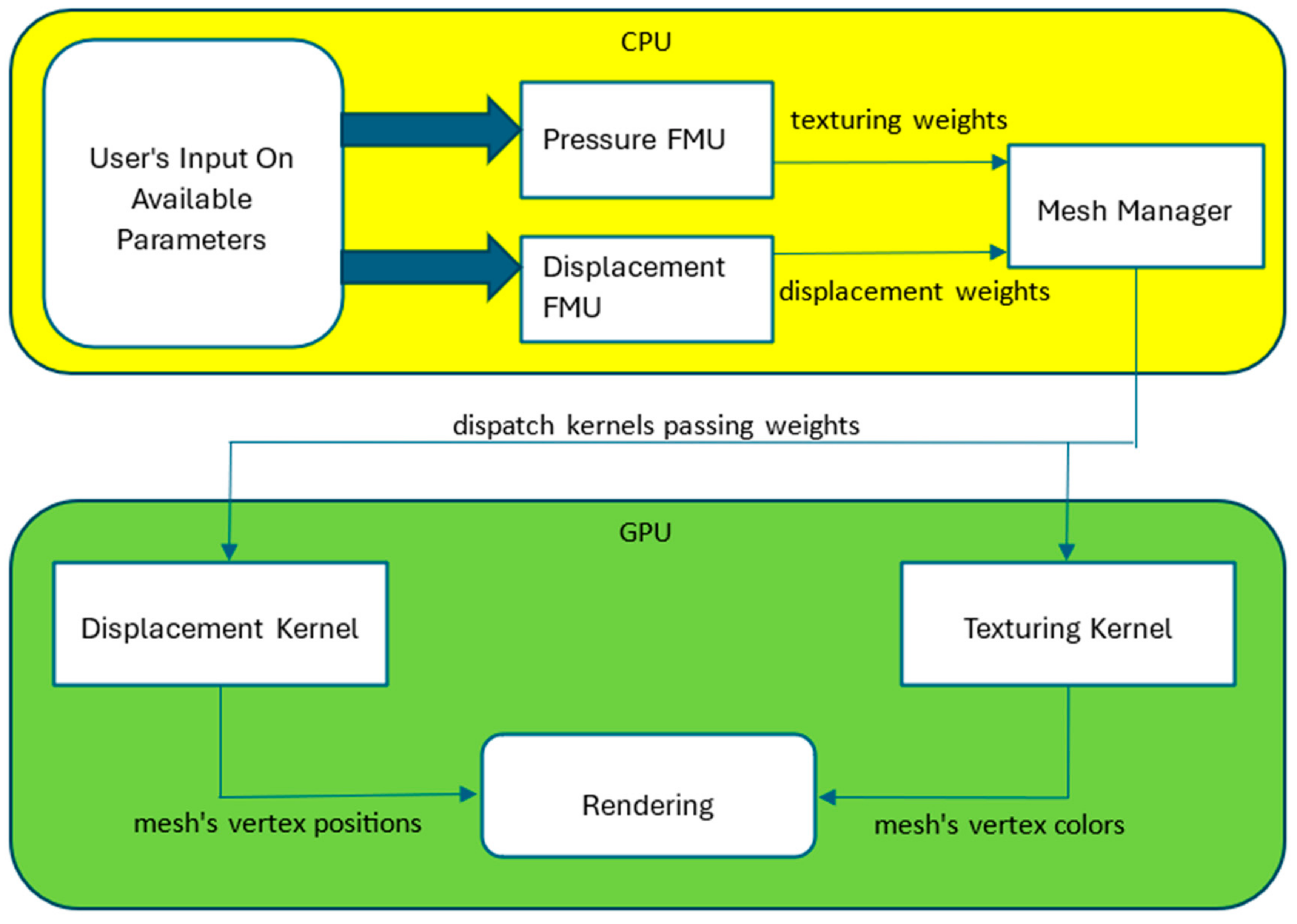
5.2.2. Visualization Module
5.2.3. Interaction Module
6. Design Example According to the Proposed Workflow
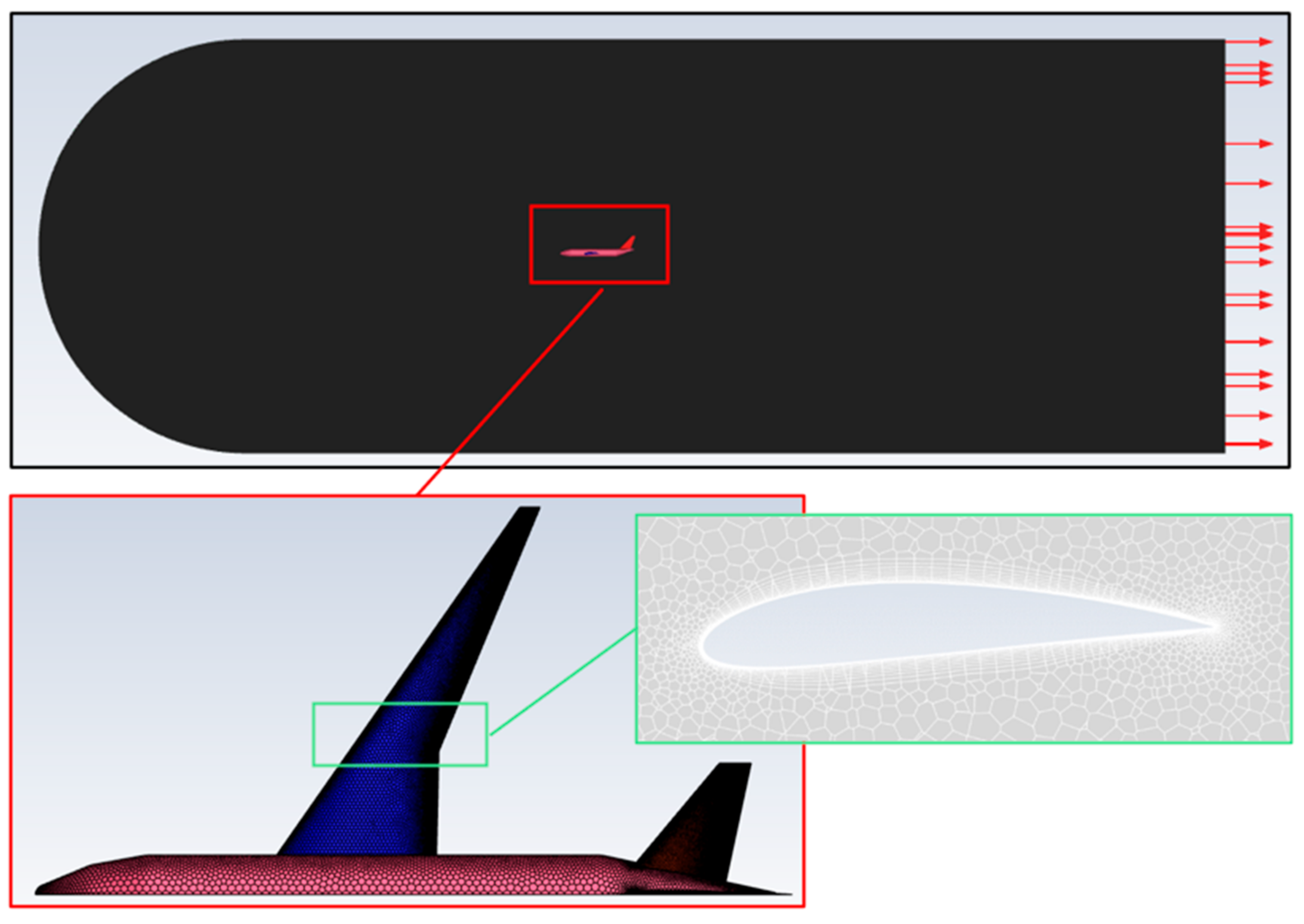
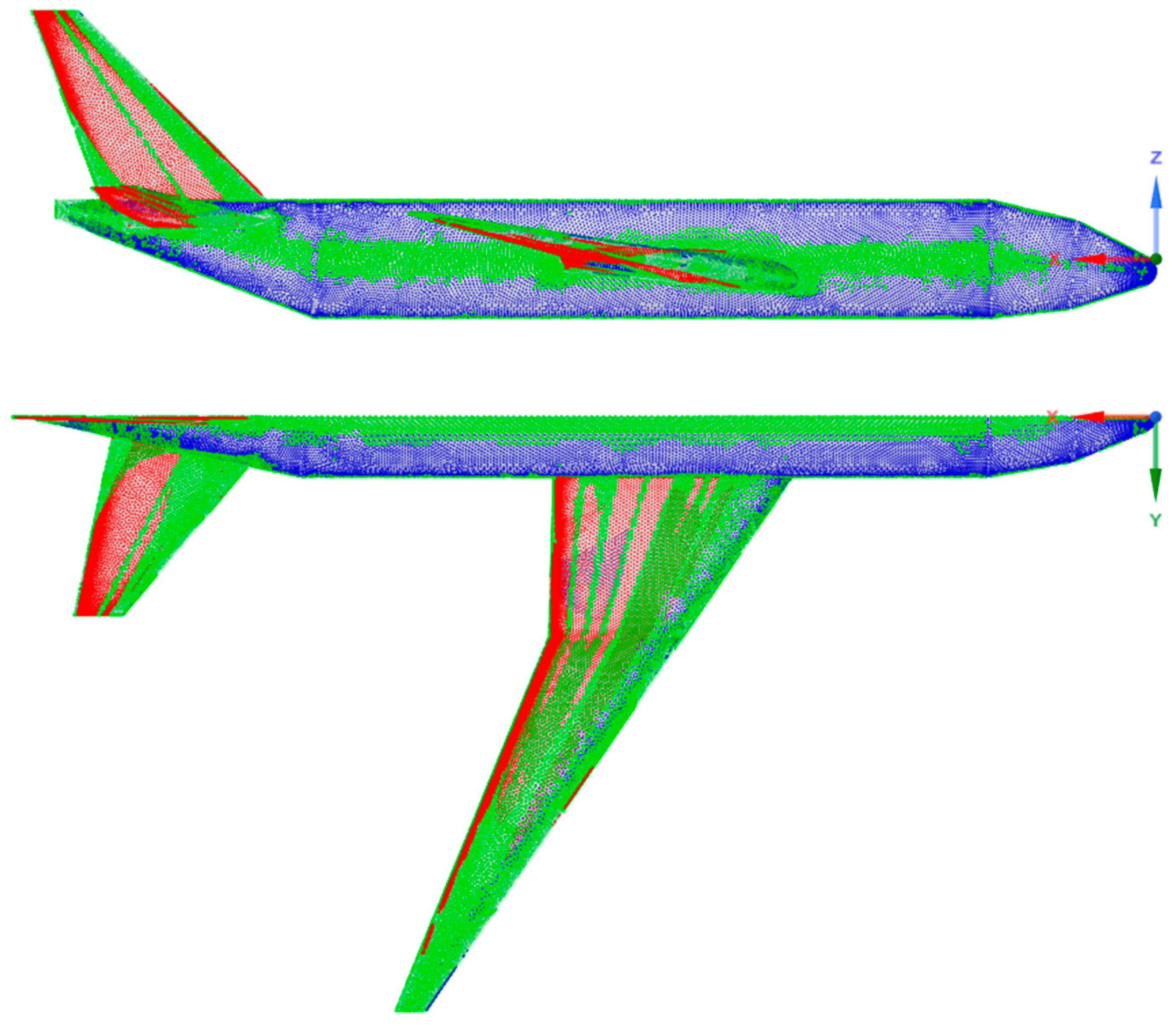
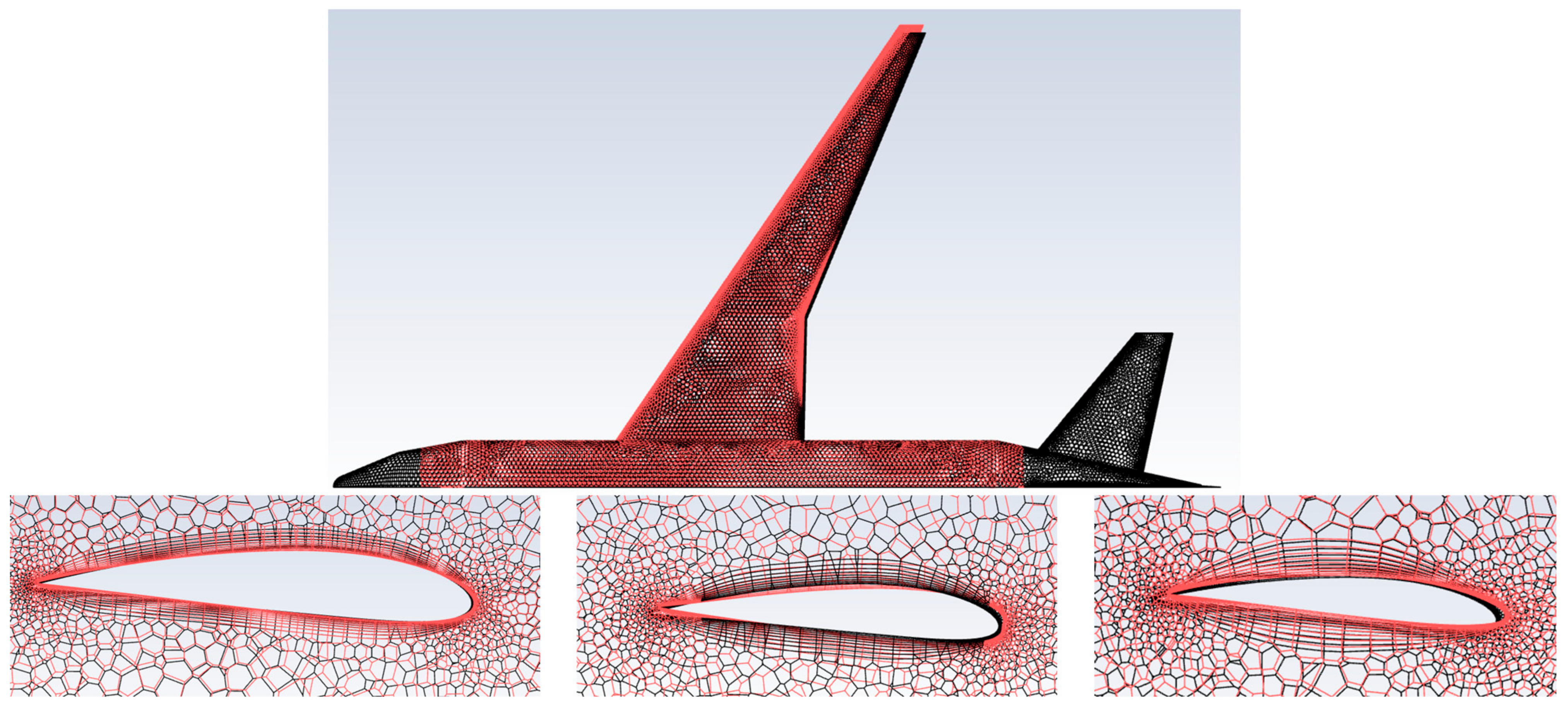
6.1. CFD Model of OPAM
- Steady-state simulation;
- Density-based solver;
- k-omega SST turbulence model;
- Air as an ideal gas with the Sutherland viscosity law;
- Boundary conditions:
- ○
- Inlet [pressure-far-field]: Mach equal to 0.7 inclined by α = 0°.
- ○
- Outlet [pressure-outlet]: Pressure and temperature standard (101,325 Pa, 298 K).
- ○
- Side [pressure-far-field]: Same conditions as the Inlet.
- ○
- Symmetry [symmetry]: Symmetry plane.
- ○
- Plane [wall].
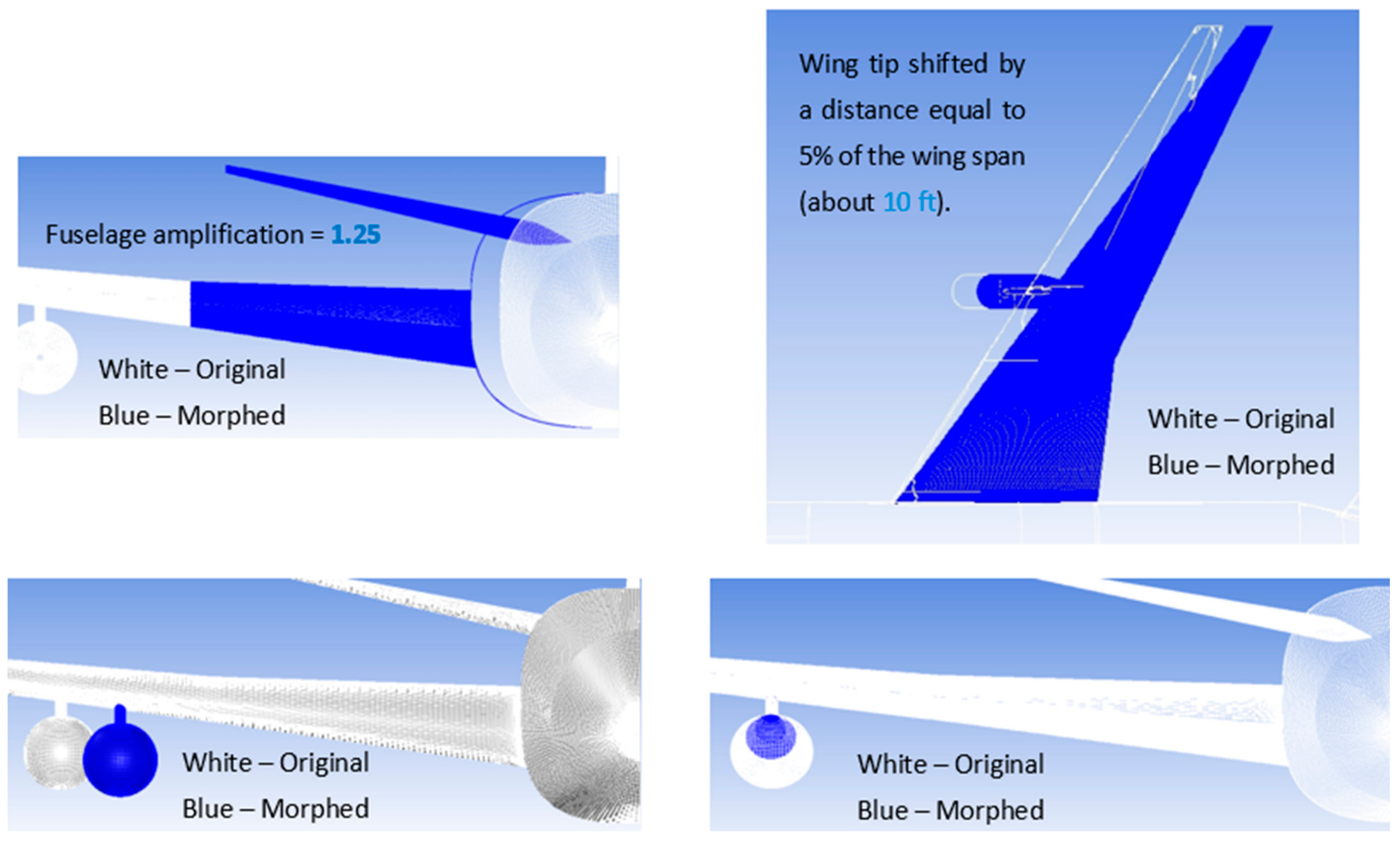
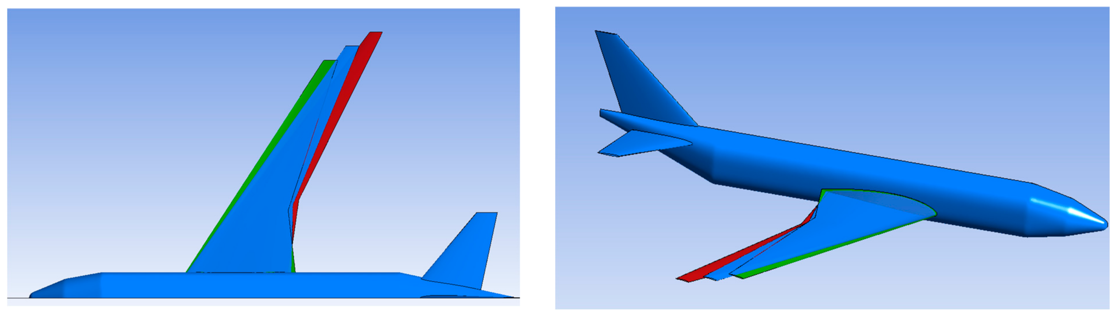
6.2. Parameters and DOE
- DP65: 8, 33, −5, 0.02, −10, 0.02
- DP66: 10, 37, −1, 0.06, −6, 0.06
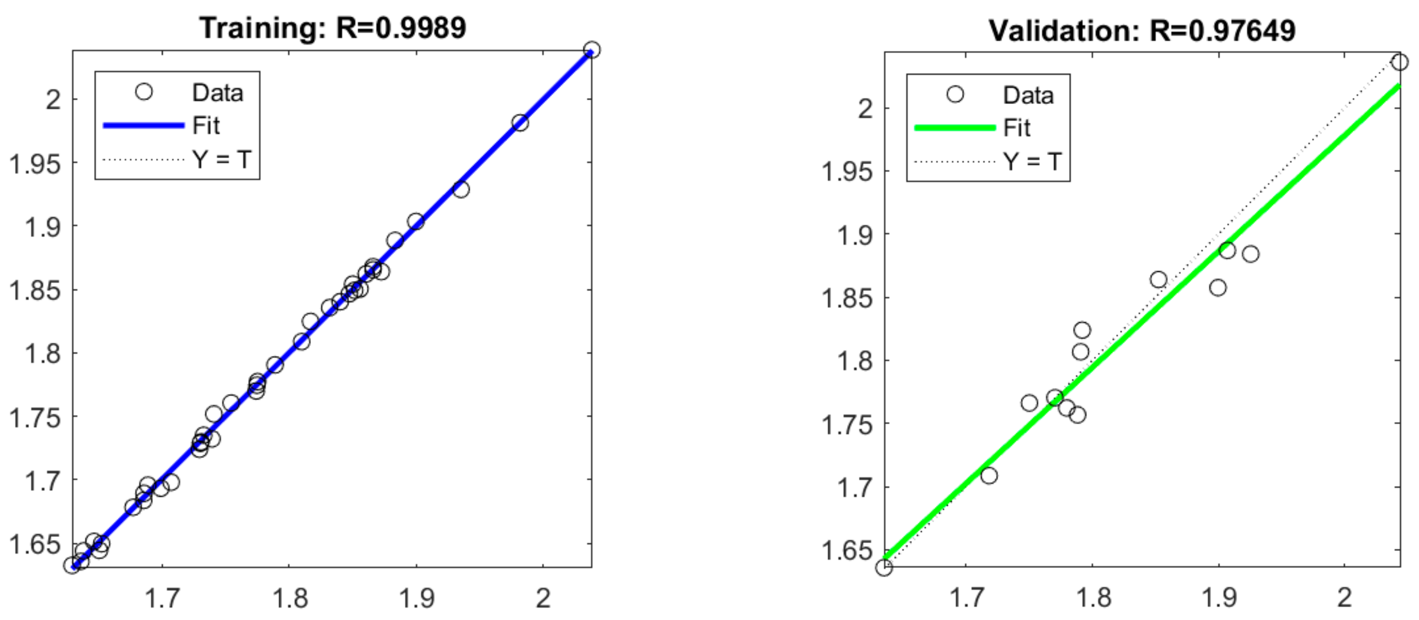
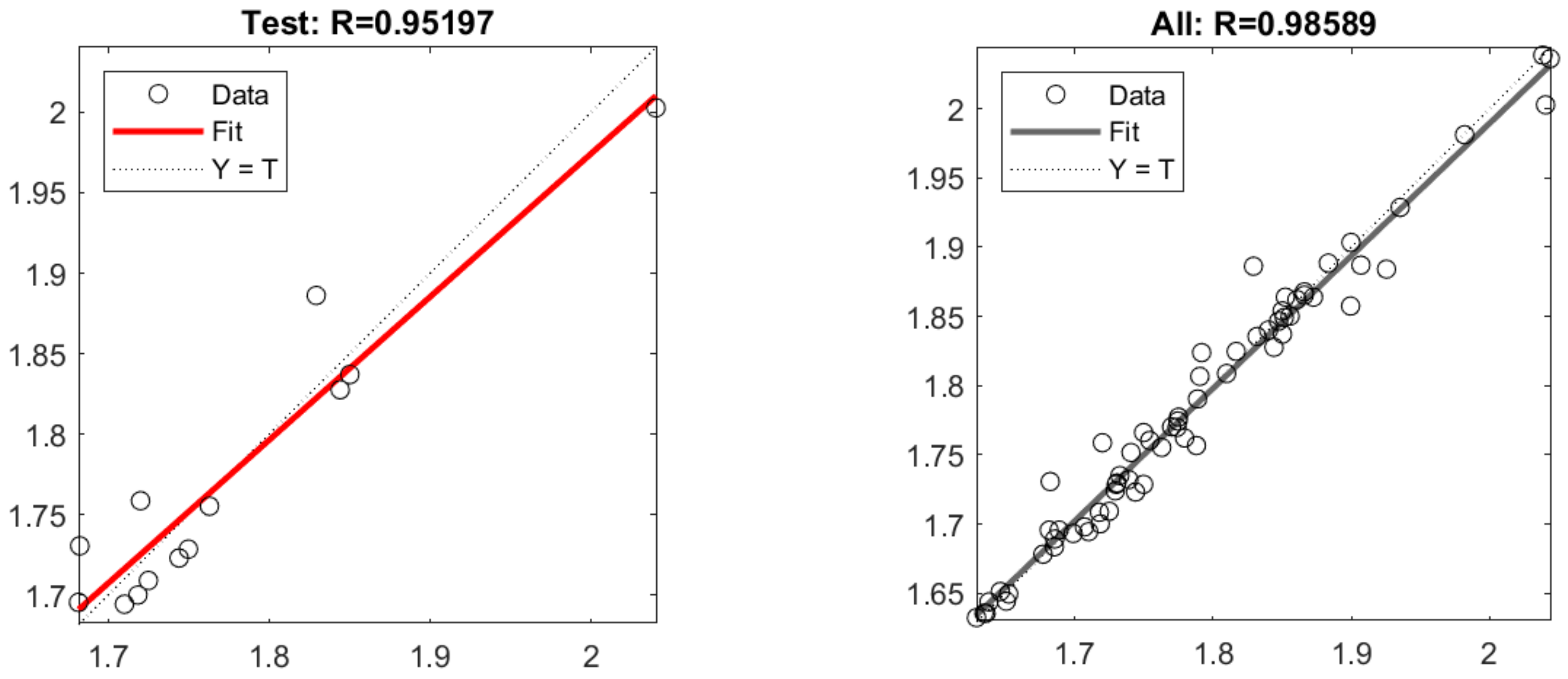
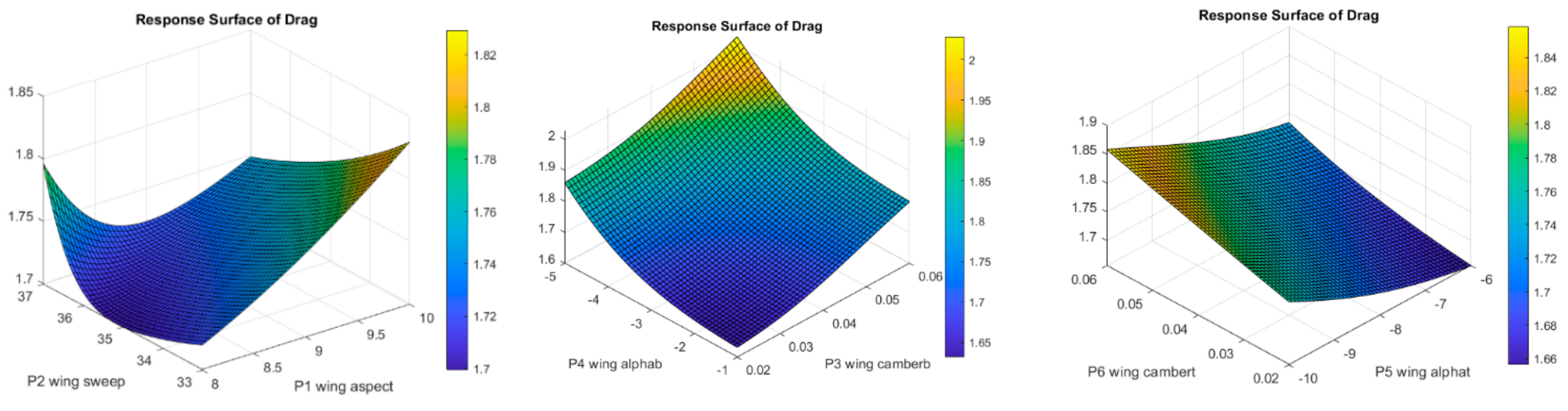
6.3. Response Surface
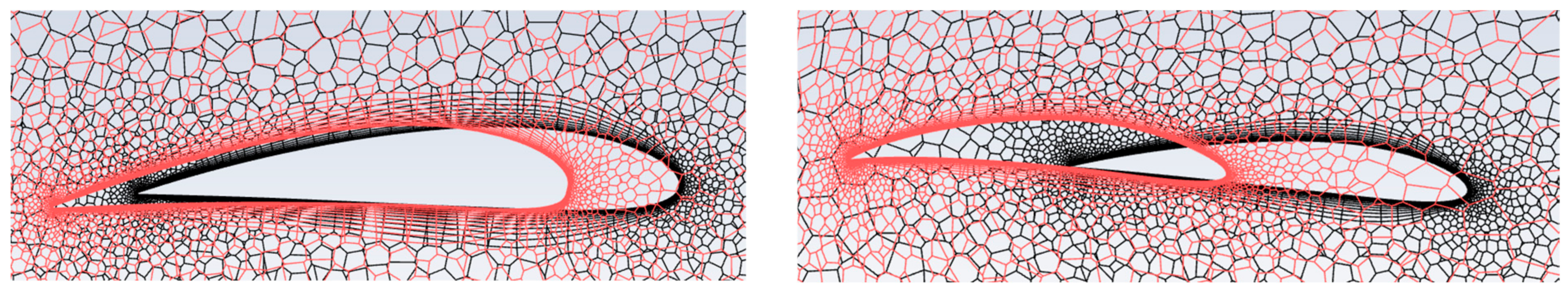
6.4. Mesh ROM
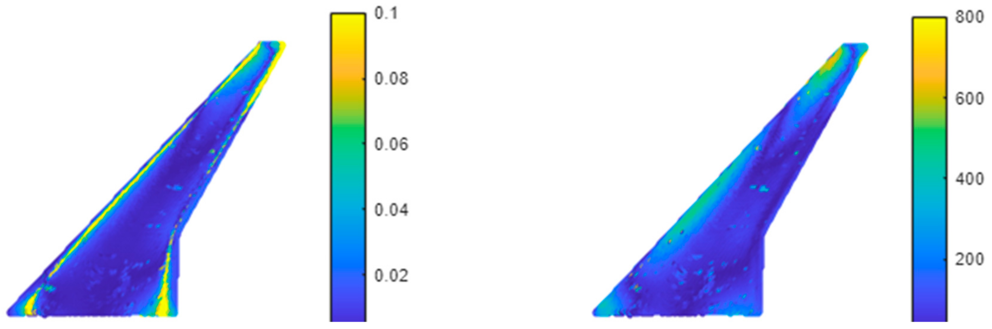
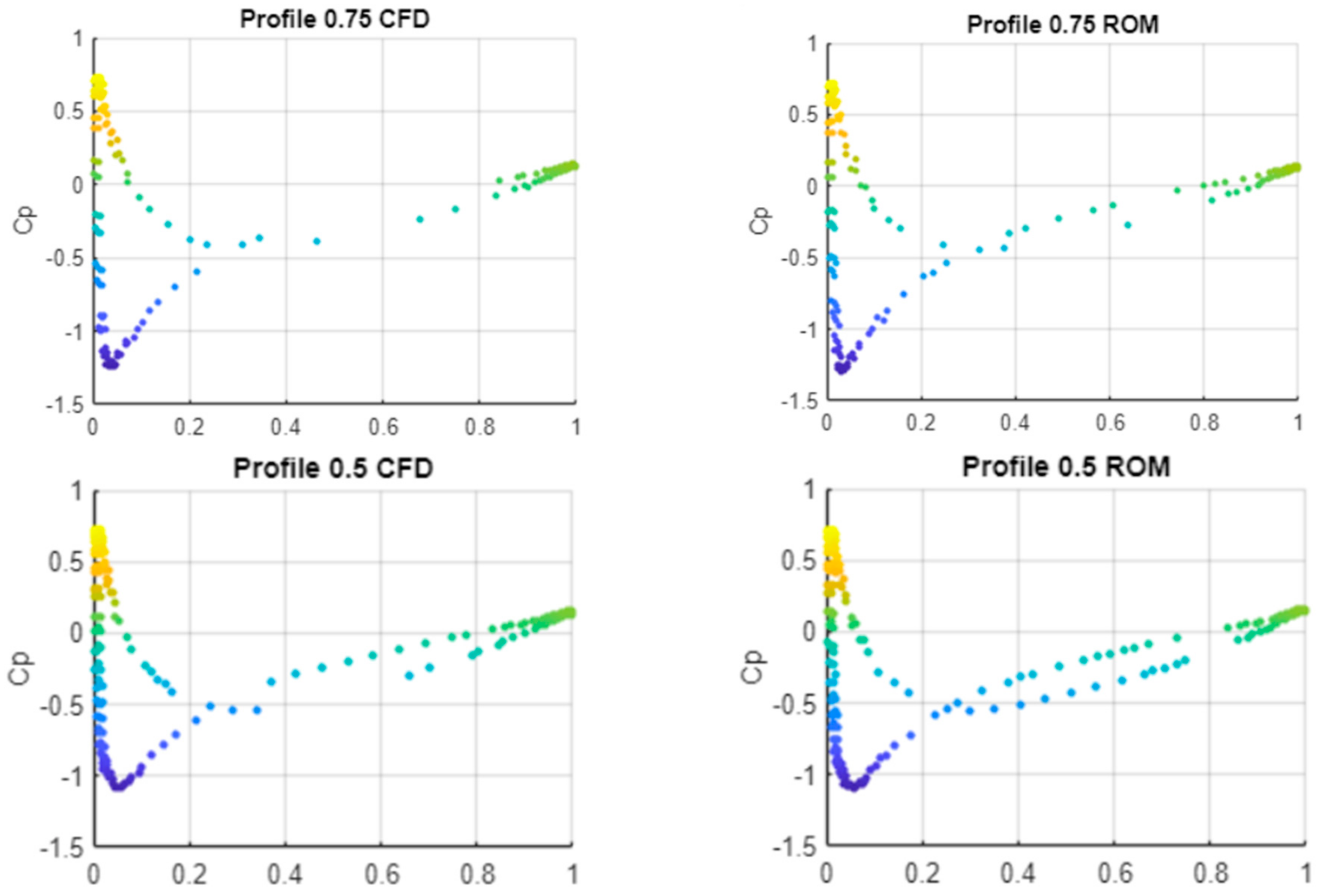
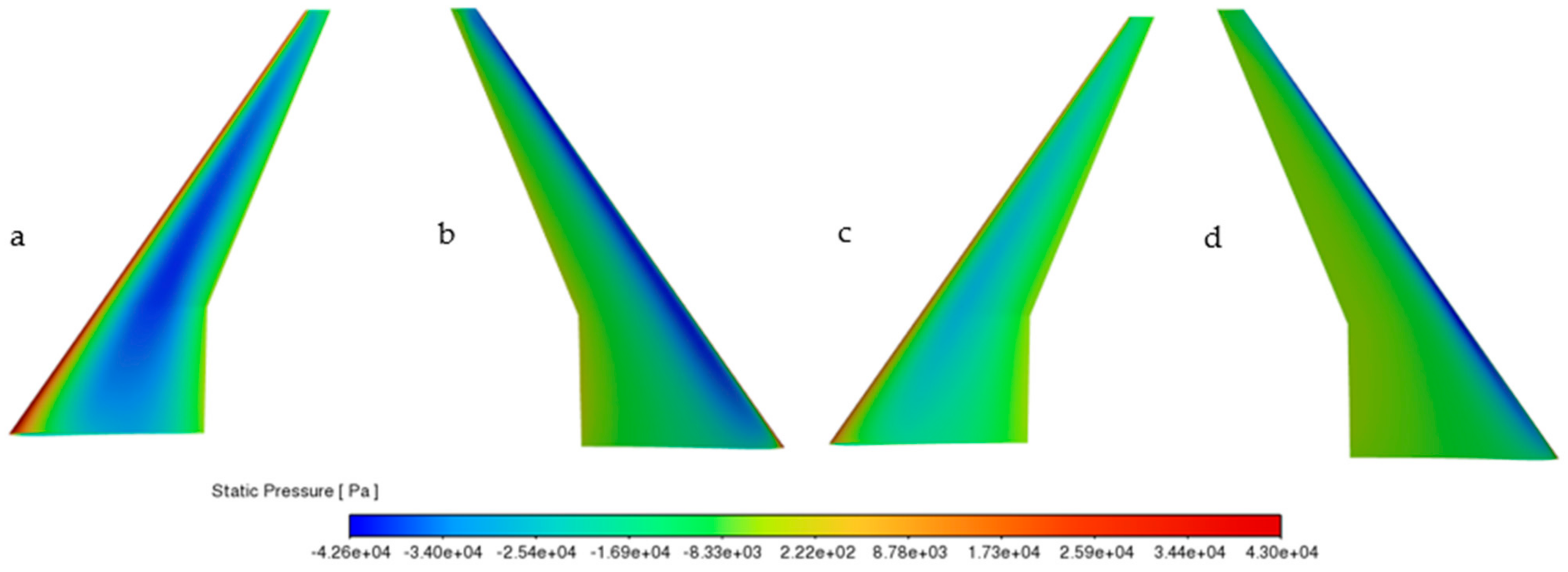
6.5. Pressure ROM
6.6. Optimization Results
6.7. VR Dashboard
7. Conclusions
Author Contributions
Funding
Institutional Review Board Statement
Informed Consent Statement
Data Availability Statement
Acknowledgments
Conflicts of Interest
Appendix A
| #DP | aspectr | sweep | alphab | camberb | alphat | cambert | Lift [N] | Drag [N] | Lift/Drag |
| 1 | 9.700 | 33.021 | −2.302 | 0.045 | −6.337 | 0.050 | 6.383 | 1.792 | 3.562 |
| 2 | 9.941 | 33.428 | −3.810 | 0.020 | −6.580 | 0.040 | 7.015 | 1.739 | 4.033 |
| 3 | 8.136 | 35.129 | −1.572 | 0.021 | −7.861 | 0.045 | 6.731 | 1.635 | 4.117 |
| 4 | 8.949 | 35.638 | −1.836 | 0.030 | −6.507 | 0.051 | 6.543 | 1.653 | 3.959 |
| 5 | 9.013 | 34.722 | −4.870 | 0.025 | −8.735 | 0.042 | 7.052 | 1.907 | 3.698 |
| 6 | 8.685 | 33.522 | −1.562 | 0.049 | −8.776 | 0.034 | 6.358 | 1.754 | 3.624 |
| 7 | 8.078 | 36.778 | −2.319 | 0.051 | −6.089 | 0.032 | 6.383 | 1.682 | 3.795 |
| 8 | 8.284 | 33.172 | −2.963 | 0.053 | −8.622 | 0.044 | 6.435 | 1.832 | 3.513 |
| 9 | 9.971 | 34.480 | −1.994 | 0.057 | −9.389 | 0.031 | 6.197 | 1.840 | 3.368 |
| 10 | 8.191 | 35.461 | −3.364 | 0.044 | −7.060 | 0.022 | 6.659 | 1.677 | 3.970 |
| 11 | 8.485 | 35.536 | −3.817 | 0.023 | −7.711 | 0.024 | 7.029 | 1.707 | 4.117 |
| 12 | 8.123 | 36.126 | −4.892 | 0.033 | −9.217 | 0.026 | 6.952 | 1.866 | 3.726 |
| 13 | 8.988 | 35.387 | −2.247 | 0.054 | −9.113 | 0.025 | 6.362 | 1.775 | 3.585 |
| 14 | 9.346 | 34.625 | −1.026 | 0.033 | −9.370 | 0.021 | 6.540 | 1.686 | 3.880 |
| 15 | 8.905 | 35.924 | −1.303 | 0.043 | −7.117 | 0.057 | 6.262 | 1.725 | 3.630 |
| 16 | 9.765 | 35.087 | −3.306 | 0.041 | −8.467 | 0.023 | 6.651 | 1.750 | 3.801 |
| 17 | 9.502 | 33.747 | −2.705 | 0.026 | −8.856 | 0.024 | 6.877 | 1.710 | 4.021 |
| 18 | 9.571 | 34.327 | −2.814 | 0.052 | −7.243 | 0.056 | 6.274 | 1.829 | 3.430 |
| 19 | 9.824 | 33.568 | −2.104 | 0.038 | −7.410 | 0.046 | 6.461 | 1.720 | 3.756 |
| 20 | 8.793 | 33.789 | −3.676 | 0.059 | −7.522 | 0.034 | 6.383 | 1.873 | 3.409 |
| 21 | 9.327 | 36.202 | −4.361 | 0.039 | −7.928 | 0.048 | 6.690 | 1.856 | 3.605 |
| 22 | 8.433 | 34.508 | −4.529 | 0.037 | −6.255 | 0.043 | 6.793 | 1.770 | 3.837 |
| 23 | 9.661 | 34.085 | −4.395 | 0.056 | −6.927 | 0.026 | 6.455 | 1.900 | 3.398 |
| 24 | 8.642 | 34.894 | −4.038 | 0.045 | −9.467 | 0.029 | 6.685 | 1.852 | 3.610 |
| 25 | 9.603 | 35.340 | −1.101 | 0.046 | −7.174 | 0.041 | 6.194 | 1.731 | 3.579 |
| 26 | 8.364 | 36.374 | −3.705 | 0.047 | −9.877 | 0.033 | 6.598 | 1.844 | 3.578 |
| 27 | 9.907 | 35.717 | −4.772 | 0.048 | −7.639 | 0.035 | 6.573 | 1.935 | 3.397 |
| 28 | 9.653 | 36.106 | −3.208 | 0.048 | −8.266 | 0.045 | 6.418 | 1.817 | 3.532 |
| 29 | 8.729 | 35.309 | −1.720 | 0.034 | −9.528 | 0.044 | 6.567 | 1.718 | 3.822 |
| 30 | 8.246 | 33.836 | −3.112 | 0.028 | −9.301 | 0.059 | 6.795 | 1.788 | 3.800 |
| 31 | 8.444 | 36.624 | −4.585 | 0.055 | −6.665 | 0.052 | 6.377 | 1.982 | 3.218 |
| 32 | 8.536 | 33.264 | −1.156 | 0.024 | −8.401 | 0.038 | 6.671 | 1.651 | 4.041 |
| 33 | 9.310 | 34.394 | −2.930 | 0.025 | −6.202 | 0.027 | 6.845 | 1.647 | 4.157 |
| 34 | 8.928 | 35.052 | −2.791 | 0.060 | −6.172 | 0.040 | 6.232 | 1.789 | 3.483 |
| 35 | 8.340 | 33.961 | −1.671 | 0.035 | −6.424 | 0.025 | 6.568 | 1.629 | 4.031 |
| 36 | 9.782 | 36.663 | −1.443 | 0.052 | −8.521 | 0.037 | 6.175 | 1.774 | 3.481 |
| 37 | 9.413 | 34.773 | −1.803 | 0.058 | −8.078 | 0.055 | 6.099 | 1.852 | 3.292 |
| 38 | 9.244 | 36.269 | −3.560 | 0.031 | −6.494 | 0.036 | 6.778 | 1.689 | 4.013 |
| 39 | 8.515 | 34.170 | −2.589 | 0.041 | −9.772 | 0.056 | 6.539 | 1.810 | 3.613 |
| 40 | 9.156 | 36.058 | −3.889 | 0.057 | −8.011 | 0.036 | 6.375 | 1.899 | 3.356 |
| 41 | 8.058 | 35.620 | −3.468 | 0.058 | −9.156 | 0.049 | 6.359 | 1.866 | 3.407 |
| 42 | 8.008 | 34.219 | −4.259 | 0.030 | −8.248 | 0.035 | 6.947 | 1.780 | 3.904 |
| 43 | 9.261 | 34.277 | −2.056 | 0.040 | −7.568 | 0.028 | 6.509 | 1.686 | 3.861 |
| 44 | 9.099 | 33.089 | −3.175 | 0.036 | −9.733 | 0.032 | 6.759 | 1.791 | 3.775 |
| 45 | 9.380 | 33.655 | −4.644 | 0.050 | −9.062 | 0.039 | 6.536 | 2.044 | 3.198 |
| 46 | 9.090 | 33.918 | −3.392 | 0.031 | −6.990 | 0.048 | 6.748 | 1.730 | 3.902 |
| 47 | 8.617 | 34.853 | −4.082 | 0.027 | −6.711 | 0.060 | 6.857 | 1.775 | 3.863 |
| 48 | 8.379 | 36.450 | −2.161 | 0.037 | −8.681 | 0.058 | 6.509 | 1.733 | 3.756 |
| 49 | 8.182 | 33.346 | −2.541 | 0.042 | −7.960 | 0.046 | 6.546 | 1.730 | 3.783 |
| 50 | 9.444 | 35.212 | −4.704 | 0.040 | −6.041 | 0.054 | 6.679 | 1.850 | 3.610 |
| 51 | 9.873 | 35.975 | −1.350 | 0.028 | −6.773 | 0.030 | 6.530 | 1.636 | 3.991 |
| 52 | 9.482 | 35.828 | −2.385 | 0.027 | −9.973 | 0.038 | 6.749 | 1.744 | 3.869 |
| 53 | 9.142 | 36.502 | −2.668 | 0.021 | −7.804 | 0.052 | 6.790 | 1.699 | 3.996 |
| 54 | 8.708 | 36.877 | −3.011 | 0.032 | −7.263 | 0.042 | 6.690 | 1.683 | 3.976 |
| 55 | 8.830 | 36.951 | −1.898 | 0.022 | −8.175 | 0.029 | 6.770 | 1.638 | 4.132 |
| 56 | 8.759 | 34.061 | −4.990 | 0.046 | −8.318 | 0.050 | 6.608 | 2.040 | 3.239 |
| 57 | 9.549 | 36.824 | −4.439 | 0.039 | −8.989 | 0.030 | 6.747 | 1.861 | 3.626 |
| 58 | 9.719 | 34.999 | −3.574 | 0.023 | −9.855 | 0.053 | 6.907 | 1.850 | 3.733 |
| 59 | 8.253 | 34.685 | −1.392 | 0.050 | −6.854 | 0.054 | 6.243 | 1.750 | 3.568 |
| 60 | 9.215 | 33.453 | −3.942 | 0.053 | −9.604 | 0.055 | 6.400 | 2.038 | 3.140 |
| 61 | 9.877 | 36.418 | −4.197 | 0.029 | −8.916 | 0.058 | 6.807 | 1.883 | 3.614 |
| 62 | 8.580 | 35.800 | −2.439 | 0.055 | −7.326 | 0.020 | 6.382 | 1.719 | 3.713 |
| 63 | 9.043 | 36.727 | −1.248 | 0.044 | −9.660 | 0.047 | 6.310 | 1.763 | 3.579 |
| 64 | 8.857 | 33.207 | −4.163 | 0.034 | −7.466 | 0.022 | 6.913 | 1.741 | 3.971 |
| 65 | 8.000 | 33.000 | −5.000 | 0.020 | −10.000 | 0.020 | 7.280 | 1.925 | 3.781 |
| 66 | 10.000 | 37.000 | −1.000 | 0.060 | −6.000 | 0.060 | 5.834 | 1.848 | 3.158 |
References
- Prusak, I.; Torlo, D.; Nonino, M.; Rozza, G. An optimisation based domain decomposition reduced order model for parameter dependent non stationary fluid dynamics problems. Comput. Math. Appl. 2024, 166, 253–268. [Google Scholar] [CrossRef]
- Geronzi, L.; Martinez, A.; Rochette, M.; Yan, K.; Bel-Brunon, A.; Haigron, P.; Escrig, P.; Tomasi, J.; Daniel, M.; Lalande, A.; et al. Computer-aided shape features extraction and regression models for predicting the ascending aortic aneurysm growth rate. Comput. Biol. Med. 2023, 162, 107052. [Google Scholar] [CrossRef]
- Kwon, T.W.; Kim, H.G.; Lee, J.S.; Jeong, C.H.; Choi, Y.C.; Ha, M.Y. AI-Enhanced design of excavator engine room cooling system using computational fluid dynamics and artificial neural networks. Case Stud. Therm. Eng. 2024, 54, 103959. [Google Scholar] [CrossRef]
- Miao, X.; Wang, Z.; Ren, S.; Zhang, L.; Li, H.; Dong, L.; Chen, D.; Hu, C. Intelligent mesh refinement based on U-NET for high-fidelity CFD simulation in numerical reactor. Nucl. Eng. Des. 2023, 411, 112411. [Google Scholar] [CrossRef]
- Mumuni, A.; Mumuni, F. Automated data processing and feature engineering for deep learning and big data applications: A survey. J. Inf. Intell. 2024, in press. [Google Scholar] [CrossRef]
- Jamshed, S. Using HPC for Computational Fluid Dynamics, Shamoon Jamshed; Elsevier: Amsterdam, The Netherlands, 2015. [Google Scholar] [CrossRef]
- Neau, H.; Ansart, R.; Baudry, C.; Fournier, Y.; Mérigoux, N.; Koren, C.; Laviéville, J.; Renon, N.; Simonin, O. HPC challenges and opportunities of industrial-scale reactive fluidized bed simulation using meshes of several billion cells on the route of Exascale. Powder Technol. 2024, 444, 120018. [Google Scholar] [CrossRef]
- Shang, Z. Impact of mesh partitioning methods in CFD for large scale parallel computing. Comput. Fluids 2014, 103, 1–5. [Google Scholar] [CrossRef]
- Koch, M.; Arlandini, C.; Antonopoulos, G.; Baretta, A.; Beaujean, P.; Bex, G.J.; Biancolini, M.E.; Celi, S.; Costa, E.; Drescher, L.; et al. HPC in the medical field: Overview and current examples. Technol. Health Care 2023, 31, 1509–1523. [Google Scholar] [CrossRef] [PubMed]
- Di Pierro, B.; Hank, S. CPU and GPU parallel efficiency of ARM based single board computing cluster for CFD applications. Comput. Fluids 2024, 272, 106187. [Google Scholar] [CrossRef]
- Ghioldi, F.; Piscaglia, F. Acceleration of supersonic/hypersonic reactive CFD simulations via heterogeneous CPU-GPU supercomputing. Comput. Fluids 2023, 266, 106041. [Google Scholar] [CrossRef]
- Voß, A.; Klimmek, T. Parametric aeroelastic modeling, maneuver loads analysis using CFD methods and structural design of a fighter aircraft. Aerosp. Sci. Technol. 2023, 136, 108231. [Google Scholar] [CrossRef]
- Zhang, L.; Chang, X.; Ma, R.; Zhao, Z.; Wang, N. A CFD-based numerical virtual flight simulator and its application in control law design of a maneuverable missile model. Chin. J. Aeronaut. 2019, 32, 2577–2591. [Google Scholar] [CrossRef]
- Viviani, A.; Aprovitola, A.; Pezzella, G.; Rainone, C. CFD design capabilities for next generation high-speed aircraft. Acta Astronaut. 2021, 178, 143–158. [Google Scholar] [CrossRef]
- Rozov, V.; Stuhlpfarrer, M.; Fernández Osma, M.; Breitsamter, C. Engine Modeling for Small-Disturbance-CFD Related to Aircraft Flutter Investigations. J. Fluids Struct. 2020, 96, 103045. [Google Scholar] [CrossRef]
- Nielsen, E.J.; Diskin, B. High-performance aerodynamic computations for aerospace applications. Parallel Comput. 2017, 64, 20–32. [Google Scholar] [CrossRef]
- Chawner, J.R.; Taylor, N.J. Progress in Geometry Modeling and Mesh Generation Toward the CFD Vision 2030. In Proceedings of the AIAA Aviation 2019 Forum, Dallas, TX, USA, 17–21 June 2019. [Google Scholar] [CrossRef]
- Hanke, J. Geometry Preparation and Mesh Generation Using Simcenter STAR-CCM+ for 4th AIAA CFD High Lift Prediction Workshop. In Proceedings of the AIAA 2022, Chicago, IL, USA, 27 June–1 July 2022. [Google Scholar] [CrossRef]
- Chawner, J.R.; Michal, T.R.; Slotnick, J.P.; Rumsey, C.L. Summary of the 1st AIAA Geometry and Mesh Generation Workshop (GMGW-1) and Future Plans. In Proceedings of the AIAA 2018, Kissimmee, FL, USA, 8–12 January 2018. [Google Scholar] [CrossRef]
- Gandhi, V.; Joe, J.; Dannenhoffer, J.F.; Dalir, H. Rapid design generation and multifidelity analysis of aircraft structures. Aerosp. Sci. Technol. 2021, 112, 106612. [Google Scholar] [CrossRef]
- Biancolini, M.E.; Viola, I.M.; Riotte, M. Sails trim optimisation using CFD and RBF mesh morphing. Comput. Fluids 2014, 93, 46–60. [Google Scholar] [CrossRef]
- Gagliardi, F.; Giannakoglou, K.C. A two–step radial basis function-based CFD mesh displacement tool. Adv. Eng. Softw. 2019, 128, 86–97. [Google Scholar] [CrossRef]
- Immonen, E. A parametric morphing method for generating structured meshes for marine free surface flow applications with plane symmetry. J. Comput. Des. Eng. 2019, 6, 348–353. [Google Scholar] [CrossRef]
- Eguea, J.P.; Bravo-Mosquera, P.D.; Catalano, F.M. Camber morphing winglet influence on aircraft drag breakdown and tip vortex structure. Aerosp. Sci. Technol. 2021, 119, 107148. [Google Scholar] [CrossRef]
- Zilong, L.; Ping, H. Accelerating unsteady aerodynamic simulations using predictive reduced-order modeling. Aerosp. Sci. Technol. 2023, 139, 108412. [Google Scholar] [CrossRef]
- Vergari, L.; Cammi, A.; Lorenzi, S. Reduced order modeling approach for parametrized thermal-hydraulics problems: Inclusion of the energy equation in the POD-FV-ROM method. Prog. Nucl. Energy 2020, 118, 103071. [Google Scholar] [CrossRef]
- Negri, E.; Fumagalli, L.; Cimino, C.; Macchi, M. FMU-supported simulation for CPS Digital Twin. Procedia Manuf. 2019, 28, 201–206. [Google Scholar] [CrossRef]
- Glujic, D.; Vukelic, G.; Bernecic, D.; Vizentin, G.; Ogrizovic, D. Coupling CFD and VR for advanced firefighting training in a virtual ship engine room. Results Eng. 2024, 24, 103025. [Google Scholar] [CrossRef]
- Capetillo, A.; Ibarra, F. Multiphase injector modelling for automotive SCR systems: A full factorial design of experiment and optimization. Comput. Math. Appl. 2017, 74, 188–200. [Google Scholar] [CrossRef]
- Wang, J.; Khan, S.A.; Yasmin, S.; Alam, M.M.; Liu, H.; Farooq, U.; Akgül, A.; Hassan, A.M. Central composite design (CCD)-Response surface methodology (RSM) for modeling and simulation of MWCNT-water nanofluid inside hexagonal cavity: Application to electronic cooling. Case Stud. Therm. Eng. 2023, 50, 103488. [Google Scholar] [CrossRef]
- Akbar, N.S.; Zamir, T.; Akram, J.; Noor, T.; Muhammad, T. Simulation of hybrid boiling nano fluid flow with convective boundary conditions through a porous stretching sheet through Levenberg Marquardt artificial neural networks approach. Int. J. Heat Mass Transf. 2024, 228, 125615. [Google Scholar] [CrossRef]
- Song, W.; Andy, J.K. Surrogate-Based Aerodynamic Shape Optimization of a Civil Aircraft Engine Nacelle. AIAA J. 2007, 45, 2565–2574. [Google Scholar] [CrossRef]
- Li, T.Z.; Yang, X.L. An efficient uniform design for Kriging-based response surface method and its application. Comput. Geotech. 2019, 109, 12–22. [Google Scholar] [CrossRef]
- Xuan-Binh Lam, D. Multidisciplinary design optimization for aircraft wing using response surface method, genetic algorithm, and simulated annealing. J. Sci. Technol. Civ. Eng. 2019, 14, 28–41. [Google Scholar] [CrossRef]
- Coppedè, A.; Gaggero, S.; Vernengo, G.; Villa, D. Hydrodynamic shape optimization by high fidelity CFD solver and Gaussian process based response surface method. Appl. Ocean Res. 2019, 90, 101841. [Google Scholar] [CrossRef]
- Ge, Y.; He, Q.; Lin, Y.; Yuan, W.; Chen, J.; Huang, S.-M. Multi-objective optimization of a mini-channel heat sink with non-uniform fins using genetic algorithm in coupling with CFD models. Appl. Therm. Eng. 2022, 207, 11812. [Google Scholar] [CrossRef]
- Bisighini, B.; Aguirre, M.; Biancolini, M.E.; Trovalusci, F.; Perrin, D.; Avril, S.; Pierrat, B. Machine learning and reduced order modelling for the simulation of braided stent deployment. Front. Physiol. 2023, 14, 1148540. [Google Scholar] [CrossRef]
- Fresca, S.; Manzoni, A. POD-DL-ROM: Enhancing deep learning-based reduced order models for nonlinear parametrized PDEs by proper orthogonal decomposition. Comput. Methods Appl. Mech. Eng. 2022, 338, 114181. [Google Scholar] [CrossRef]
- Lorenzi, S.; Cammi, A.; Luzzi, L.; Rozza, G. POD-Galerkin method for finite volume approximation of Navier–Stokes and RANS equations. Comput. Methods Appl. Mech. Eng. 2016, 311, 151–179. [Google Scholar] [CrossRef]
- Santolamazza, A.; Groth, C.; Introna, V.; Porziani, S.; Scarpitta, F.; Urso, G.; Valentini, P.P.; Costa, E.; Ferrante, E.; Sorrentino, S.; et al. A Digital Shadow cloud-based application to enhance quality control in manufacturing. IFAC-PapersOnLine 2020, 53, 10579–10584. [Google Scholar] [CrossRef]
- Yan, Z.; Gong, J.; Louste, C.; Wu, J.; Fang, J. Modal analysis of EHD jets through the SVD-based POD technique. J. Electrost. 2023, 126, 103858. [Google Scholar] [CrossRef]
- Mifsud, M.; Vendl, A.; Hansen, L.-U.; Görtz, S. Fusing wind-tunnel measurements and CFD data using constrained gappy proper orthogonal decomposition. Aerosp. Sci. Technol. 2019, 86, 312–326. [Google Scholar] [CrossRef]
- Casella, F.; Leva, A. Modelling and Simulation of Thermal Power Generation Systems with Modelica: 20 Years of Experience with the ThermoPower Library. IFAC-PapersOnLine 2024, 58, 227–234. [Google Scholar] [CrossRef]
- Masoom, A.; Guironnet, A.; Zeghaida, A.A.; Ould-Bachir, T.; Mahseredjian, J. Modelica-based simulation of electromagnetic transients using Dynaωo: Current status and perspectives. Electr. Power Syst. Res. 2021, 197, 107340. [Google Scholar] [CrossRef]
- D’Amelio, E.L.; Bascetta, L.; Cucci, D.A.; Matteucci, M.; Bardaro, G. A Modelica simulator to support the development of the control system of an autonomous All-Terrain mobile robot. IFAC-PapersOnLine 2015, 48, 274–279. [Google Scholar] [CrossRef]
- Hinkelman, K.; Wang, J.; Zuo, W.; Gautier, A.; Wetter, M.; Fan, C.; Long, N. Modelica-based modeling and simulation of district cooling systems: A case study. Appl. Energy 2022, 311, 118654. [Google Scholar] [CrossRef]
- Woeber, C.; Masters, J.S.; McDaniel, D.R. Summary of Exascale and Remeshing Efforts for the Second Geometry and Mesh Generation Workshop. In Proceedings of the AIAA 2019, Dallas, TX, USA, 17–21 June 2019. [Google Scholar] [CrossRef]
- Dannenhoffer, J.F. Analysis of GMGW2 Case 3: Design Variations. In Proceedings of the AIAA 2019, Dallas, TX, USA, 17–21 June 2019. [Google Scholar] [CrossRef]
- Haimes, R.; Drela, M. On The Construction of Aircraft Conceptual Designs. In Proceedings of the AIAA 2012, Garden Grove, CA, USA, 19–21 June 2012. [Google Scholar] [CrossRef]
- Cella, U.; Biancolini, M.E. RBF Morph. 2019. Available online: https://www.rbf-morph.com/wp-content/uploads/2019/02/GMGW2-Case3-Wade.pdf (accessed on 1 November 2024).
- Karman, S.; Wyman, N. Automatic Unstructured Mesh Generation with Geometry Attribution. In Proceedings of the AIAA 2019, Dallas, TX, USA, 17–21 June 2019. [Google Scholar] [CrossRef]
- Chan, W.M.; Pandyay, S.A.; Haimes, R. Automation of Overset Structured Surface Mesh Generation on Complex Geometries. In Proceedings of the AIAA 2019, Dallas, TX, USA, 17–21 June 2019. [Google Scholar] [CrossRef]
- Magri, G.; Lopez, A.; Della Barba, F. Ottimizzazione Aerodinamica di un Velivolo Mediante CAD Parametrico e Mesh Morphing. Master’s Thesis, Univeristy of Padova, Padua, Italy, 2023. [Google Scholar]
- Gagliardi, F.; Giannakoglou, K.C. RBF-based morphing of B-Rep models for use in aerodynamic shape optimization. Adv. Eng. Softw. 2019, 138, 102724. [Google Scholar] [CrossRef]
- Cadquery Documentation. Available online: https://cadquery.readthedocs.io/en/latest/ (accessed on 26 December 2024).
- Viisainen, J.V.; Yu, F.; Codolini, A.; Chen, S.; Harper, L.T.; Sutcliffe, M.P.F. Rapidly predicting the effect of tool geometry on the wrinkling of biaxial NCFs during composites manufacturing using a deep learning surrogate model. Compos. Part B Eng. 2023, 253, 110536. [Google Scholar] [CrossRef]
- Automatic modeling of aircraft external geometries for preliminary design workflows. Aerosp. Sci. Technol. 2020, 98, 105667. [CrossRef]
- Guo, S.; Duan, F.; Tang, H.; Lim, S.C.; Yip, M.S. Multi-objective optimization for centrifugal compressor of mini turbojet engine. Aerosp. Sci. Technol. 2014, 39, 414–425. [Google Scholar] [CrossRef]
- Goldbach, A.-K.; Lázaro, C. CAD-integrated parametric design and analysis of lightweight shell structures. Structures 2024, 64, 106566. [Google Scholar] [CrossRef]
- Available online: https://dev.opencascade.org/doc/overview/html/ (accessed on 26 December 2024).
- Available online: https://www.opencascade.com/products/cad-builder/ (accessed on 26 December 2024).
- Sieger, D.; Menzel, S.; Botsch, M. On Shape Deformation Techniques for Simulation-Based Design Optimization. In New Challenges in Grid Generation and Adaptivity for Scientific Computing; SEMA SIMAI Springer Series; Springer: Cham, Switzerland, 2015. [Google Scholar] [CrossRef]
- Iordanis, I.; Koukouvinos, C.; Silou, I. On the efficacy of conditioned and progressive Latin hypercube sampling in supervised machine learning. Appl. Numer. Math. 2024, 208, 256–270. [Google Scholar] [CrossRef]
- Guilbaud, T.; Fiorina, C.; Lorenzi, S.; Scolaro, A.; Carminati, F.; Maire, D.; Pautz, A. Investigating the Functional Mock-up Interface as a Coupling Framework for the multi-fidelity analysis of nuclear reactors. Prog. Nucl. Energy 2024, 169, 105022. [Google Scholar] [CrossRef]


| Number of faces | 4,979,888 |
| Number of cells | 957,205 |
| Number of nodes | 3,366,691 |
| Min. Orthogonal Quality | 1.50172 × 10⁻¹ |
| Max. Aspect Ratio | 1.38865 × 10+2 |
| y+ | <10 |
| Number of faces | 4,979,888 |
| Aspect R | Sweep | Alpha B | Camber B | Alpha T | Camber T | |
|---|---|---|---|---|---|---|
| Range | 8 ÷ 10 | 33 ÷ 37 | −5 ÷ −1 | 0.02 ÷ 0.06 | −10 ÷ −6 | 0.02 ÷ 0.06 |
| Baseline | 9 | 35 | −3 | 0.04 | −8 | 0.04 |
| Min Orthogonal Quality | DP |
|---|---|
| 1.45437 × 10⁻¹ | baseline |
| 8.80044 × 10⁻² | 1 |
| 9.94842 × 10⁻² | 10 |
| 9.51205 × 10⁻² | 20 |
| 1.02042 × 10⁻¹ | 30 |
| 1.02038 × 10⁻¹ | 40 |
| 9.15076 × 10⁻² | 50 |
| 9.12111 × 10⁻² | 60 |
| 5.18119 × 10⁻² | 65 |
| 9.16307 × 10⁻² | 66 |
| Observations | MSE | R | |
|---|---|---|---|
| Train | 40 (60%) | 2.15 × 10⁻⁵ | 0.9989 |
| Validation | 13 (20%) | 5.37 × 10⁻⁴ | 0.9765 |
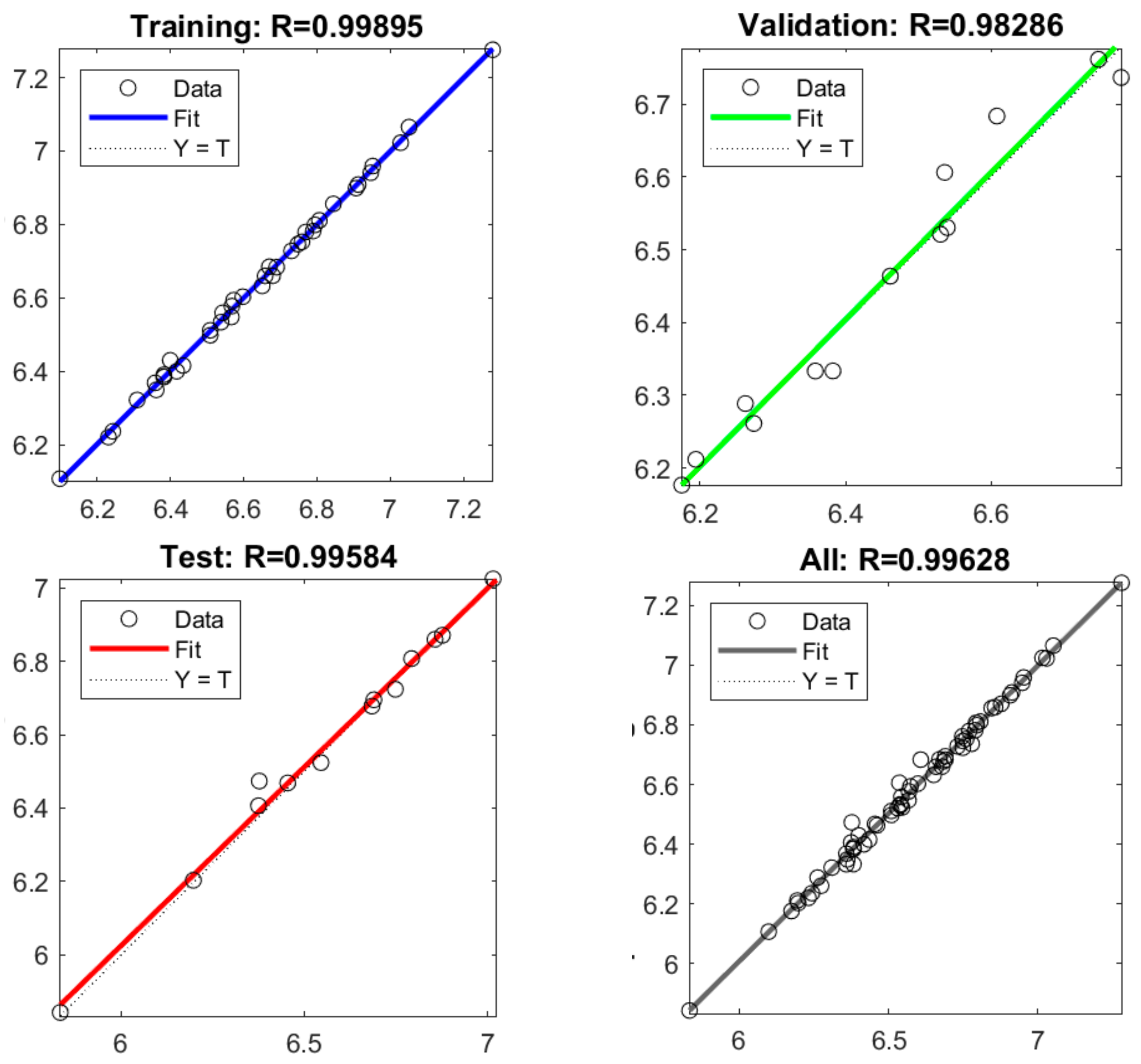
| Observations | MSE | R | |
|---|---|---|---|
| Train | 40 (60%) | 0.0001 | 0.9989 |
| Validation | 13 (20%) | 0.0013 | 0.9829 |
| Aspect R | Sweep | Alpha B | Camber B | Alpha T | Camber T | |
|---|---|---|---|---|---|---|
| Range | 8 ÷ 10 | 33 ÷ 37 | −5 ÷ −1 | 0.02 ÷ 0.06 | −10 ÷ −6 | 0.02 ÷ 0.06 |
| Optimized | 9.31 | 34.39 | −2.93 | 0.025 | −6.2 | 0.027 |
| Cl | Cd | Eff | |
|---|---|---|---|
| Baseline | 0.505 | 0.134 | 3.77 |
| Optimized | 0.535 (+6%) | 0.129 (−4%) | 4.15 (+10%) |
Disclaimer/Publisher’s Note: The statements, opinions and data contained in all publications are solely those of the individual author(s) and contributor(s) and not of MDPI and/or the editor(s). MDPI and/or the editor(s) disclaim responsibility for any injury to people or property resulting from any ideas, methods, instructions or products referred to in the content. |
© 2025 by the authors. Licensee MDPI, Basel, Switzerland. This article is an open access article distributed under the terms and conditions of the Creative Commons Attribution (CC BY) license (https://creativecommons.org/licenses/by/4.0/).
Share and Cite
Lopez, A.; Biancolini, M.E. Development of a Reduced Order Model-Based Workflow for Integrating Computer-Aided Design Editors with Aerodynamics in a Virtual Reality Dashboard: Open Parametric Aircraft Model-1 Testcase. Appl. Sci. 2025, 15, 846. https://doi.org/10.3390/app15020846
Lopez A, Biancolini ME. Development of a Reduced Order Model-Based Workflow for Integrating Computer-Aided Design Editors with Aerodynamics in a Virtual Reality Dashboard: Open Parametric Aircraft Model-1 Testcase. Applied Sciences. 2025; 15(2):846. https://doi.org/10.3390/app15020846
Chicago/Turabian StyleLopez, Andrea, and Marco E. Biancolini. 2025. "Development of a Reduced Order Model-Based Workflow for Integrating Computer-Aided Design Editors with Aerodynamics in a Virtual Reality Dashboard: Open Parametric Aircraft Model-1 Testcase" Applied Sciences 15, no. 2: 846. https://doi.org/10.3390/app15020846
APA StyleLopez, A., & Biancolini, M. E. (2025). Development of a Reduced Order Model-Based Workflow for Integrating Computer-Aided Design Editors with Aerodynamics in a Virtual Reality Dashboard: Open Parametric Aircraft Model-1 Testcase. Applied Sciences, 15(2), 846. https://doi.org/10.3390/app15020846