Transient Horizontal Response of a Pipe Pile in Saturated Soil with a Flexible Support at the Pile Head

Abstract

This study examines the horizontal transient response of pipe piles in saturated soil, assuming a two-stage equivalent linear relationship between the bending moment and the rotation at the pile head. The potential function is introduced, and the three-dimensional wave equation for saturated soils is decoupled using operator decomposition and the method of separation of variables. By applying the appropriate initial and boundary conditions, the horizontal lateral forces on the pile from both the surrounding soil and the soil within the pile shaft are calculated. The pipe pile is modeled as a Timoshenko beam. Continuity conditions at the pile–-soil interface are applied, and a time-domain solution for horizontal transient vibrations is derived. This solution accounts for various pile top constraint conditions and is obtained through the inverse Laplace transform. Validation against existing results demonstrates the accuracy of the proposed model. Finally, a parametric study investigates the effects of factors such as impact load, permeability, pile diameter, and pile head constraints on pile displacement.

1. Introduction

The dynamic behavior of pile foundations under lateral loads is a critical topic in soil–structure interaction research, with wide applications in offshore wind farms and seismic design [1,2]. In engineering practice, transient loads such as earthquakes, wave impacts, and traffic vibrations pose significant challenges to the safety and performance of pile foundations [3,4,5,6]. Accurate prediction of the dynamic response of pile foundations under these loads is essential for ensuring reliable designs. However, existing studies face limitations in analyzing the transient horizontal response of soil–pile systems, highlighting the need for further improvement to advance both theory and application in this field.

Frequency-domain methods are widely used for studying the dynamic behavior of pile foundations, particularly under steady-state load conditions [7,8]. M. H. El Naggar et al. [9,10,11] derived frequency-domain solutions for the vertical and lateral vibrations of piles using the dynamic Winkler model, while Y. C. Han et al. [12,13] developed impedance functions for radially inhomogeneous soil layers based on the boundary layer model and investigated pile vertical vibration characteristics. Despite their effectiveness in analyzing periodic steady-state loads, frequency-domain methods exhibit significant limitations in capturing the short-term dynamic responses caused by transient loads, particularly during the complex behavior in the initial loading phase [14,15].

To address this, time-domain methods have been introduced into pile–soil interaction research, offering a new approach for transient dynamic response analysis [16]. Nogami and Konagai [16] first proposed a time-domain analytical method based on the closed-form solutions by Novak et al. [17], who studied the transient vertical response of elastic piles in homogeneous and inhomogeneous soils. By dividing the pile–soil system into horizontal layers and using the transfer matrix method, this approach significantly simplified the computational process. Subsequently, this method was extended to analyze the dynamic behavior of pile–soil systems under transient lateral loads, representing a major breakthrough in the field [18]. However, most existing time-domain methods assume idealized pile head boundary conditions, such as fully fixed or fully free, without adequately addressing the flexible constraints commonly encountered in real-world engineering scenarios.

Pile head rotation under flexible constraints is a common issue in structures such as offshore jacket foundations, pile-supported wind turbines, and precast tubular piles with inadequate anchorage. Such rotation can occur either within the pile cap or within the superstructure. Even in pile groups with rigid pile head connections, axial deformation of the piles can induce rotation at the pile head [19,20]. In these cases, the pile head behaves as a flexible restraint, between fully fixed (zero rotation) and fully free conditions, with its rotational stiffness significantly influencing the horizontal load-bearing characteristics of the pile [2021]. Catal et al. [21] modeled the semi-rigid pile head connection using linear springs and analyzed the natural frequencies and relative stiffness of partially embedded piles. Sadek et al. [22] investigated the effects of different pile head boundary conditions (fixed and hinged) on the seismic response of piles under harmonic earthquake waves. Jiang Lihong et al. [23] proposed a simplified calculation method for horizontally loaded piles under varying rotational stiffness using the p–y curve method, while Yang et al. [24] studied the effects of rotational stiffness and yielding moment on the horizontal transient response of piles under Rayleigh wave excitation.

This paper proposes a transient dynamic analysis framework for studying the horizontal dynamics of tubular piles in saturated soils with flexible constraints at the pile head. The framework integrates Biot’s equations, the Timoshenko beam model, and a time-domain solution method. By applying the Laplace transform, the differential equations are transformed into algebraic equations, significantly reducing computational complexity. Compared to traditional frequency-domain methods, the time-domain approach captures the dynamic characteristics of transient loads more intuitively, particularly the complex responses during the initial loading phase. Furthermore, the framework incorporates the fluid–solid coupling effects of saturated soils and employs a three-dimensional wave equation to describe the soil’s dynamic behavior, providing a more realistic representation of soil–pile interaction dynamics.

The objectives of this study are as follows: (1) to propose a time-domain solution method by integrating Biot’s equations and the Timoshenko beam model to analyze the transient horizontal response of tubular piles in saturated soils under flexible constraints at the pile head, (2) to validate the proposed method through numerical simulations and parameter analysis, investigating the effects of key parameters (such as permeability coefficient, pile diameter, and load type) on pile displacement and stress characteristics, and (3) to provide theoretical guidance for the engineering design of pile foundations in complex soil conditions, thereby advancing research in soil–structure dynamics.

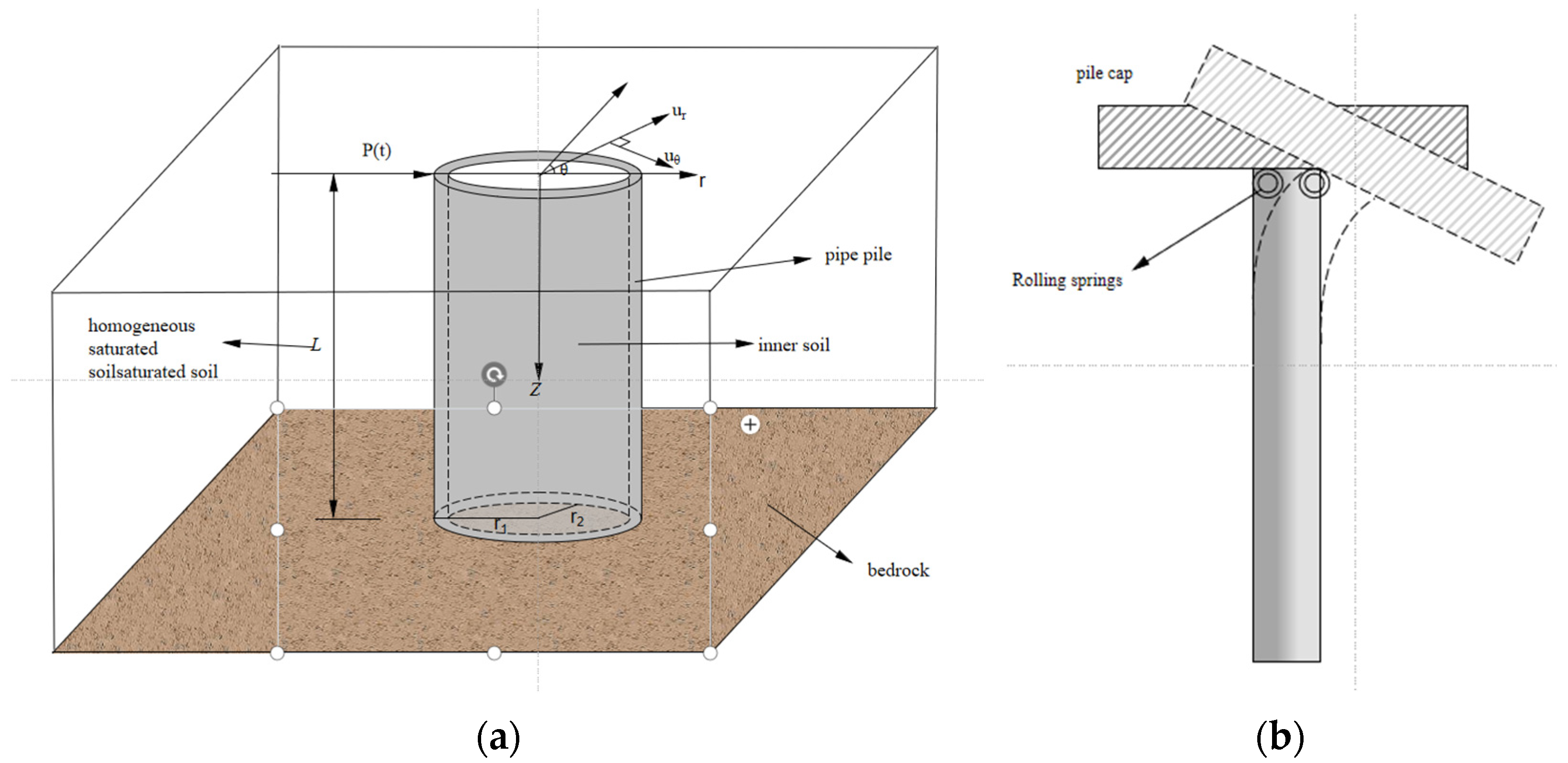
2. Mathematical Model and Assumptions

Figure 1 shows the computational model for the horizontal transient vibration of a pipe pile in saturated soil and the pile inner soil is assumed to be flush with the pile top. A horizontal transient load, p(t), is applied at the pile head in the roz plane. The following assumptions are made in the analysis:

• Both the surrounding soil and the pile core soil are homogeneous, isotropic, and modeled as a saturated biphasic elastic medium.
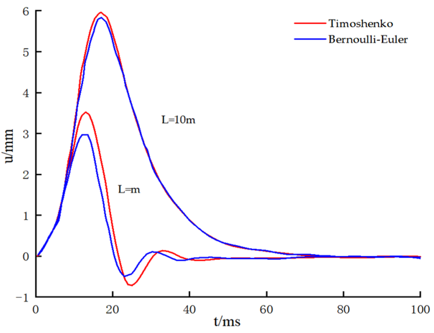
• The pile is modeled as an elastic, uniform cross-section annular shaft, using the Timoshenko beam theory to simulate its behavior. Pile shear deformation is considered, and the pile base is fixed.
• The pile–soil vibrations are assumed to involve small deformations, with perfect contact between the pile and the surrounding soil. The displacement and force at the pile–soil interface are continuous, and the interface is impermeable.
• During the horizontal vibration, the vertical displacement of the soil skeleton and pore fluid is much smaller than the lateral displacement of the pile. The effect of lateral friction along the pile surface is also small and thus neglected in the analysis. This study is limited to the scope of elastic dynamics and does not explore dynamic strength considerations. For simplicity, the effects of strain rate caused by impact loads are excluded from the analysis [25].

3. Formulation and Solution of Governing Equations

3.1. Fundamental Equations

For horizontal transient vibrations, assuming negligible vertical displacements of both the soil and pore water, the three-dimensional equation of motion for saturated soil in a cylindrical coordinate system under non-axisymmetric conditions is expressed as [26]:

$$G_i{\nabla }^2{u}_{ri}+\left({\lambda }_i+G_i\right){\displaystyle \frac{\mathsf{\partial }{e}_i}{\mathsf{\partial }r}}-{\displaystyle \frac{G_i}{r^2}}\left(2{\displaystyle \frac{\mathsf{\partial }{u}_{\theta i}}{\mathsf{\partial }\theta }}+u_{ri}\right)-\alpha {\displaystyle \frac{\mathsf{\partial }{p}_f}{\mathsf{\partial }r}}+G_i{\displaystyle \frac{{\mathsf{\partial }}^2{u}_{ri}}{\mathsf{\partial }{z}^2}}={\rho }_i{\ddot{u}}_{ri}+{\rho }_f{\ddot{w}}_{ri}$$

(1)

$$G_i{\nabla }^2{u}_{\theta i}+\left({\lambda }_i+G_i\right){\displaystyle \frac{1}{r}}{\displaystyle \frac{\mathsf{\partial }{e}_i}{\mathsf{\partial }\theta }}-{\displaystyle \frac{G_i}{r^2}}\left(u_{\theta i}-2{\displaystyle \frac{\mathsf{\partial }{u}_{ri}}{\mathsf{\partial }\theta }}\right)-\alpha {\displaystyle \frac{1}{r}}{\displaystyle \frac{\mathsf{\partial }{p}_f}{\mathsf{\partial }\theta }}+G_i{\displaystyle \frac{{\mathsf{\partial }}^2{u}_{\theta i}}{\mathsf{\partial }{z}^2}}={\rho }_i{\ddot{u}}_{\theta i}+{\rho }_f{\ddot{w}}_{\theta i}$$

(2)

The governing equation for fluid motion in the soil is:

$$-{\displaystyle \frac{\mathsf{\partial }{p}_f}{\mathsf{\partial }r}}={\displaystyle \frac{1}{k_d^{\prime }}}{\dot{w}}_{ri}+{\rho }_f{\ddot{u}}_{ri}+{\displaystyle \frac{{\rho }_f}{n}}{\ddot{w}}_{ri}$$

(3)

$$-{\displaystyle \frac{1}{r}}{\displaystyle \frac{\mathsf{\partial }{p}_f}{\mathsf{\partial }\theta }}={\displaystyle \frac{1}{k_d^{\prime }}}{\dot{w}}_{\theta i}+{\rho }_f{\ddot{u}}_{\theta i}+{\displaystyle \frac{{\rho }_f}{n}}{\ddot{w}}_{\theta i}$$

(4)

The governing equation for soil seepage is:

$$M_i\left({\displaystyle \frac{\mathsf{\partial }{\dot{w}}_{ri}}{\mathsf{\partial }r}}+{\displaystyle \frac{{\dot{w}}_{ri}}{r}}+{\displaystyle \frac{1}{r}}{\displaystyle \frac{\mathsf{\partial }{\dot{w}}_{\theta i}}{\mathsf{\partial }\theta }}\right)+{\alpha }_i{M}_i\left({\displaystyle \frac{\mathsf{\partial }{\dot{u}}_{ri}}{\mathsf{\partial }r}}+{\displaystyle \frac{{\dot{u}}_{ri}}{r}}+{\displaystyle \frac{1}{r}}{\displaystyle \frac{\mathsf{\partial }{\dot{u}}_{\theta i}}{\mathsf{\partial }\theta }}\right)=-{\dot{p}}_f$$

(5)

In the equation,

$$k_{di}^{\prime }=k_{di}/\left({\rho }_{f}g\right),{\nabla }^2={\mathsf{\partial }}^2/\mathsf{\partial }{r}^2+\mathsf{\partial }/\left(r\mathsf{\partial }r\right)+{\mathsf{\partial }}^2/\left(r^2\mathsf{\partial }{\theta }^2\right),$$

$$e_i=\mathsf{\partial }{u}_{ri}/\mathsf{\partial }r+u_{ri}/r+\mathsf{\partial }{u}_{\theta i}/r\mathsf{\partial }\theta ,K_{\mathrm{b}i}={\lambda }_i+(2/3)\times G_i,{\alpha }_i=1-K_{bi}/K_{si},M={K_{si}}^2/(K_{di}-K_{bi}),$$

$$K_{di}=K_{si}[1+n_i(K_{si}/K_{fi}-1)],{\rho }_i=(1-n_i){\rho }_{si}+n_i{\rho }_{fi}.$$

The shear effects must be considered when analyzing the impact response of structures [27,28]. Consequently, the Timoshenko beam model, which accounts for shear deformation in the pile body, was employed in the following analysis. The governing differential equations of motion for this model are expressed as follows:

$$k^{\prime }{G}_{p}A\left({\displaystyle \frac{\mathsf{\partial }\theta }{\mathsf{\partial }z}}-{\displaystyle \frac{{\mathsf{\partial }}^{2}u}{\mathsf{\partial }{z}^2}}\right)+{\rho }_{p}A{\displaystyle \frac{{\mathsf{\partial }}^{2}u}{\mathsf{\partial }{t}^2}}=-\left(q_{n1}+q_{n2}\right)$$

(6)

$$k^{\prime }{G}_{p}A\left({\theta }_p-{\displaystyle \frac{\mathsf{\partial }{u}_p}{\mathsf{\partial }z}}\right)+{\rho }_p{I}_p{\displaystyle \frac{{\mathsf{\partial }}^2{\theta }_p}{\mathsf{\partial }{t}^2}}-E_p{I}_p{\displaystyle \frac{{\mathsf{\partial }}^2{\theta }_p}{\mathsf{\partial }{z}^2}}=0$$

(7)

In the equation,

$$k^{\prime }={\displaystyle \frac{3}{4}}{\displaystyle \frac{r_1^2+r_2^2}{r_1^2+r_1{r}_2+r_2^2}}$$

3.2. Boundary Conditions

Boundary Conditions for Saturated Soil Layer:

(1)

At an infinite horizontal distance, the soil displacement approaches zero, while at r = 0, the displacement remains finite.

$$u_{ri}\left(\infty ,\theta ,z,t\right)=u_{\theta i}\left(\infty ,\theta ,z,t\right)=0$$

(8)

$$u_{ri}\left(0,\theta ,z,t\right)=u_{\theta i}\left(0,\theta ,z,t\right)\ne \infty$$

(9)

(2)

The horizontal displacement of the soil at the base of the rigid foundation is set to zero.

$$u_{ri}\left(r,\theta ,L,t\right)=u_{\theta i}\left(r,\theta ,L,t\right)=0$$

(10)

(3)

Under the assumption that the vertical displacement of the soil is negligible, the condition of zero surface stress yields the following:

$${\left.{\displaystyle \frac{\mathsf{\partial }{u}_{ri}}{\mathsf{\partial }z}}\right|}_{z=0}=0$$

(11)

The conditions at the pile–soil interface are defined as:

(1)

The pile and soil are in full contact, with no slip or separation at the interface.

$${\left.u_{ri}\right|}_{r=r_i}={\left.u_p\right|}_{r=r_i}\cos \theta$$

(12)

$${\left.u_{\theta i}\right|}_{r=r_i}=-{\left.u_p\right|}_{r=r_i}\sin \theta$$

(13)

(2)

The pile–soil interface is impermeable.

$${\left.w_{ri}\right|}_{r=r_i}=0$$

(14)

The boundary conditions for the pipe pile are as follows:

(1)

Boundary Conditions at the Pile Top:

$${\left.E_p{I}_p{\displaystyle \frac{\mathsf{\partial }\theta }{\mathsf{\partial }z}}\right|}_{z=0}=0$$

(15)

$${\left.k^{\prime }{G}_{p}A\left(\theta -{\displaystyle \frac{\mathsf{\partial }u}{\mathsf{\partial }z}}\right)\right|}_{z=0}=p\left(t\right)$$

(16)

(2)

Rigid Support Conditions at the Pile Base:

$${\left.u\right|}_{z=L}=0$$

(17)

$${\left.\theta \right|}_{z=L}=0$$

(18)

3.3. The Solution to the Equations for the Surrounding Soil and Core Soil of the Pile

At the circular hole corresponding to the outer diameter of the pipe pile, the resultant force q_n1, arising from the radial and tangential stresses within a unit thickness of the soil layer, passes through the center of the hole. By convention, q_n1 is defined as positive when its direction aligns with the motion, leading to:

$$q_{n1}={\displaystyle {\int }_0^{2\pi }{\left.\left[-\left({{\sigma }_{r1}}^{\prime }-P_1\right)\cos \theta +{\tau }_{r\theta 1}\sin \theta \right]\right|}_{r=r_1}\cdot r_{1}d\theta }$$

(19)

$$q_{n2}={\displaystyle {\int }_0^{2\pi }{\left.\left[\left({{\sigma }_{r2}}^{\prime }-P_2\right)\cos \theta -{\tau }_{r\theta 2}\sin \theta \right]\right|}_{r=r_2}\cdot r_{2}d\theta }$$

(20)

In the above equations:

$${{\sigma }_{ri}}^{\prime }={\lambda }_i{e}_i+2G_i\mathsf{\partial }{u}_{ri}/\mathsf{\partial }r,{\tau }_{r\theta i}=G_i\left(\mathsf{\partial }{u}_{\theta i}/\mathsf{\partial }r+\mathsf{\partial }{u}_{ri}/r\mathsf{\partial }\theta -u_{\theta i}/r\right)$$

$$P_i=-{\alpha }_i{M}_i{e}_i+M_i{\epsilon }_i,e_i=\mathsf{\partial }{u}_{ri}/\mathsf{\partial }r+u_{ri}/r+\mathsf{\partial }{u}_{\theta i}/r\mathsf{\partial }\theta ,{\epsilon }_i=-(\mathsf{\partial }{w}_{ri}/\mathsf{\partial }r+w_{ri}/r+\mathsf{\partial }{w}_{\theta i}/r\mathsf{\partial }\theta ).$$

The displacements of the solid skeleton and pore water can be determined by solving Equations (1)–(5) using the potential function method, the method of separation of variables, or the direct solution method [29]. Substituting the expressions for each variable into Equation (19) and performing a Laplace transform yield the following result:

$${\overline{q}}_{n1}={\displaystyle \sum _{n=1}^{\infty }{A}_n{A}_{1n}ch\left(g_{n}z\right)}$$

(21)

The pile–soil interface conditions can be incorporated into the series form of the displacement expressions to derive the solution: g_n = (2n − 1)πi/(2L), n = 1, 2, 3……

$$\begin{array}{l}{A}_n=-\pi r_1\left({\lambda }_1+2G+{\alpha }_1{M}_1+{\alpha }_{11}{M}_1\right){\beta }_{11}^2{K}_1\left({\beta }_{11}{r}_1\right)\\ -\pi r_1\left[\left({\lambda }_1+2G+{\alpha }_1{M}_1+{\alpha }_{12}{M}_1\right)B_1{\beta }_{12}^2{K}_1\left({\beta }_{12}{r}_1\right)+G_1{B}_2{\beta }_{13}^2{K}_1\left({\beta }_{13}{r}_1\right)\right]\end{array}$$

$$d_{11}={\displaystyle \frac{\left({\lambda }_1+2G_1+{\alpha }_1^2{M}_1\right)\left(s/k_d^{\prime }+{\rho }_f{s}^2/n\right)-\left(G_1{h}_{11}^2-s^2{\rho }_1\right)M_1-2{\rho }_f{\alpha }_1{M}_1{s}^2}{M_1\left({\lambda }_1+2G_1\right)}}$$

$$d_{12}={\displaystyle \frac{\left(s^2{\rho }_1-G_1{h}_{11}^2\right)\left(s/k_d^{\prime }+{\rho }_f{s}^2/n\right)-{\rho }_f^2{s}^4}{M_1\left({\lambda }_1+2G_1\right)}}$$

$${\beta }_{11}^2={\displaystyle \frac{d_{11}+\sqrt{d_{11}^2-4d_{12}}}{2}},{\beta }_{12}^2={\displaystyle \frac{d_{11}-\sqrt{d_{11}^2-4d_{12}}}{2}},{\beta }_{13}^2={\displaystyle \frac{-\left(G_1{h}_{11}^2-{\rho }_1{s}^2\right)\left(s/k_d^{\prime }+{\rho }_f{s}^2/n\right)-{\rho }_f^2{s}^4}{G_1\left(s/k_d^{\prime }+{\rho }_f{s}^2/n\right)}}$$

$${\alpha }_{11}={\displaystyle \frac{-{\alpha }_1{M}_1{\beta }_{11}^2+{\rho }_f{s}^2}{M_1{\beta }_{11}^2-(s/k_d^{\prime }+{\rho }_f{s}^2/n)}},{\alpha }_{12}={\displaystyle \frac{-{\alpha }_1{M}_1{\beta }_{12}^2+{\rho }_f{s}^2}{M_1{\beta }_{12}^2-(s/k_d^{\prime }+{\rho }_f{s}^2/n)}},{\alpha }_{13}={\displaystyle \frac{-{\rho }_f{s}^2}{s/k_d^{\prime }+{\rho }_f{s}^2/n}}$$

$$B_1={\displaystyle \frac{r_1{\beta }_{13}{K}_2\left({\beta }_{13}{r}_1\right){\alpha }_{11}{\beta }_{11}\left(K_0\left({\beta }_{11}{r}_1\right)+K_2\left({\beta }_{11}{r}_1\right)\right)-2{\beta }_{11}{K}_2\left({\beta }_{11}{r}_1\right){\alpha }_{13}{K}_1\left({\beta }_{13}{r}_1\right)}{2{\beta }_{12}{K}_2\left({\beta }_{12}{r}_1\right){\alpha }_{13}{K}_1\left({\beta }_{13}{r}_1\right)-r_1{\beta }_{13}{K}_2\left({\beta }_{13}{r}_1\right){\alpha }_{12}{\beta }_{12}\left(K_0\left({\beta }_{12}{r}_1\right)+K_2\left({\beta }_{12}{r}_1\right)\right)}}$$

$$B_2={\displaystyle \frac{-r_1{\beta }_{12}{K}_2\left({\beta }_{12}{r}_1\right){\alpha }_{11}{\beta }_{11}\left(K_0\left({\beta }_{11}{r}_1\right)+K_2\left({\beta }_{11}{r}_1\right)\right)-r_1{\beta }_{11}{K}_2\left({\beta }_{11}{r}_1\right){\alpha }_{12}{\beta }_{12}\left(K_0\left({\beta }_{12}{r}_1\right)+K_2\left({\beta }_{12}{r}_1\right)\right)}{r_1{\beta }_{13}{K}_2\left({\beta }_{13}{r}_1\right){\alpha }_{12}{\beta }_{12}\left(K_0\left({\beta }_{12}{r}_1\right)+K_2\left({\beta }_{12}{r}_1\right)\right)-2{\beta }_{12}{K}_2\left({\beta }_{12}{r}_1\right){\alpha }_{13}{K}_1\left({\beta }_{13}{r}_1\right)}}$$

Applying the same analytical method as for the soil surrounding the pile, while ensuring meticulous attention to boundary conditions and directional considerations, we substitute the variable expressions into Equation (20). By performing a Laplace transform and systematically rearranging the terms, the resulting expression is derived as follows:

$${\overline{q}}_{n2}={\displaystyle \sum _{n=1}^{\infty }{C}_n{C}_{1n}ch\left(g_{n}z\right)}$$

(22)

The coefficient C_1n can be determined by substituting the conditions at the pile–soil interface into the series representation of the displacement expression.

$$\begin{gathered} \begin{array}{l}{C}_n=\pi r_2\left({\lambda }_2+2G_2+{\alpha }_2{M}_2+{\alpha }_{21}{M}_2\right){\beta }_{21}^2{I}_1\left({\beta }_{21}{r}_2\right)\\ +\pi r_2\left[\left({\lambda }_2+2G_2+{\alpha }_2{M}_2+{\alpha }_{22}{M}_2\right)D_1{\beta }_{22}^2{I}_1\left({\beta }_{22}{r}_2\right)+G_2{D}_2{\beta }_{23}^2{I}_1\left({\beta }_{23}{r}_2\right)\right]\end{array} \\ {\beta }_{11}^2={\displaystyle \frac{d_{11}+\sqrt{d_{11}^2-4d_{12}}}{2}},{\beta }_{12}^2={\displaystyle \frac{d_{11}-\sqrt{d_{11}^2-4d_{12}}}{2}},{\beta }_{23}^2={\displaystyle \frac{-\left(G_2{h}_{21}^2-{\rho }_2{s}^2\right)\left(s/k_d^{\prime }+{\rho }_f{s}^2/n\right)-{\rho }_f^2{s}^4}{G_2\left(s/k_d^{\prime }+{\rho }_f{s}^2/n\right)}} \end{gathered}$$

$$\begin{gathered} d_{21}={\displaystyle \frac{\left({\lambda }_2+2G_2+{\alpha }_2^2{M}_2\right)\left(s/k_d^{\prime }+{\rho }_f{s}^2/n\right)-\left(G_2{h}_{21}^2-s^2{\rho }_2\right)M_2-2{\rho }_f{\alpha }_2{M}_2{s}^2}{M_2\left({\lambda }_2+2G_2\right)}} \\ {d}_{22}={\displaystyle \frac{\left(s^2{\rho }_2-G_2{h}_{21}^2\right)\left(s/k_d^{\prime }+{\rho }_f{s}^2/n\right)-{\rho }_f^2{s}^4}{M_2\left({\lambda }_2+2G_2\right)}} \\ {\alpha }_{21}={\displaystyle \frac{-{\alpha }_2{M}_2{\beta }_{21}^2+{\rho }_f{s}^2}{M_2{\beta }_{21}^2-(s/k_d^{\prime }+{\rho }_f{s}^2/n)}},{\alpha }_{22}={\displaystyle \frac{-{\alpha }_2{M}_2{\beta }_{22}^2+{\rho }_f{s}^2}{M_2{\beta }_{22}^2-(s/k_d^{\prime }+{\rho }_f{s}^2/n)}},{\alpha }_{23}={\displaystyle \frac{-{\rho }_f{s}^2}{s/k_d^{\prime }+{\rho }_f{s}^2/n}} \end{gathered}$$

$$\begin{gathered} D_1=={\displaystyle \frac{-r_2{\beta }_{23}{I}_2\left({\beta }_{23}{r}_2\right){\alpha }_{21}{\beta }_{21}\left(I_0\left({\beta }_{21}{r}_2\right)+I_2\left({\beta }_{21}{r}_2\right)\right)-2{\beta }_{21}{I}_2\left({\beta }_{21}{r}_2\right){\alpha }_{23}{I}_1\left({\beta }_{23}{r}_2\right)}{2{\beta }_{22}{I}_2\left({\beta }_{22}{r}_2\right){\alpha }_{23}{I}_1\left({\beta }_{23}{r}_2\right)+r_2{\beta }_{23}{I}_2\left({\beta }_{23}{r}_2\right){\alpha }_{22}{\beta }_{22}\left(I_0\left({\beta }_{22}{r}_2\right)+I_2\left({\beta }_{22}{r}_2\right)\right)}} \\ {D}_2=={\displaystyle \frac{r_2{\beta }_{22}{I}_2\left({\beta }_{22}{r}_2\right){\alpha }_{21}{\beta }_{21}\left(I_0\left({\beta }_{21}{r}_2\right)+I_2\left({\beta }_{21}{r}_2\right)\right)-r_2{\beta }_{21}{I}_2\left({\beta }_{21}{r}_2\right){\alpha }_{22}{\beta }_{22}\left(I_0\left({\beta }_{22}{r}_2\right)+I_2\left({\beta }_{22}{r}_2\right)\right)}{-r_2{\beta }_{23}{I}_2\left({\beta }_{23}{r}_2\right){\alpha }_{22}{\beta }_{22}\left(I_0\left({\beta }_{22}{r}_2\right)+I_2\left({\beta }_{22}{r}_2\right)\right)-2{\beta }_{22}{I}_2\left({\beta }_{22}{r}_2\right){\alpha }_{23}{I}_1\left({\beta }_{23}{r}_2\right)}} \end{gathered}$$

3.4. Solving the Equation of Pile Vibration

After applying the Laplace transform to Equations (6) and (7), the resulting expressions are obtained as:

$$k^{\prime }{G}_{p}A\left({\displaystyle \frac{\mathsf{\partial }\overline{\theta }}{\mathsf{\partial }z}}-{\displaystyle \frac{{\mathsf{\partial }}^2\overline{u}}{\mathsf{\partial }{z}^2}}\right)+{\rho }_{p}A{s}^2\overline{u}=-\left({\overline{q}}_{n1}+{\overline{q}}_{n2}\right)$$

(23)

$$k^{\prime }{G}_{p}A\left(\overline{\theta }-{\displaystyle \frac{\mathsf{\partial }\overline{u}}{\mathsf{\partial }z}}\right)+{\rho }_p{I}_p{s}^2\overline{\theta }-E_p{I}_p{\displaystyle \frac{{\mathsf{\partial }}^2\overline{\theta }}{\mathsf{\partial }{z}^2}}=0$$

(24)

where $\overline{u}$ and $\overline{\theta }$ represent the Laplace transform quantities of u and θ, respectively.

$${\displaystyle \frac{{\mathsf{\partial }}^4\overline{u}}{\mathsf{\partial }{z}^4}}+\mathrm{B}{\displaystyle \frac{{\mathsf{\partial }}^2\overline{u}}{\mathsf{\partial }{z}^2}}+C\overline{u}={\displaystyle \frac{1}{k^{\prime }{G}_{p}A}}{\displaystyle \frac{{\mathsf{\partial }}^2\left({\overline{q}}_{n1}+{\overline{q}}_{n2}\right)}{\mathsf{\partial }{z}^2}}-\left({\displaystyle \frac{{\rho }_p{I}_p{s}^2}{k^{\prime }{G}_{p}A}}+1\right){\displaystyle \frac{{\overline{q}}_{n1}+{\overline{q}}_{n2}}{E_p{I}_p}}$$

(25)

$${\displaystyle \frac{{\mathsf{\partial }}^4\overline{\theta }}{\mathsf{\partial }{z}^4}}+\mathrm{B}{\displaystyle \frac{{\mathsf{\partial }}^2\overline{\theta }}{\mathsf{\partial }{z}^2}}+C{\overline{\theta }}_p=-{\displaystyle \frac{1}{E_p{I}_p}}{\displaystyle \frac{\mathsf{\partial }\left({\overline{q}}_{n1}+{\overline{q}}_{n2}\right)}{\mathsf{\partial }z}}$$

(26)

$$B=-\left({\displaystyle \frac{{\rho }_p{s}^2}{E_p}}+{\displaystyle \frac{{\rho }_p{s}^2}{k^{\prime }{G}_p}}\right),C={\displaystyle \frac{{\rho }_p^2{s}^4}{k^{\prime }{G}_p{E}_p}}+{\displaystyle \frac{{\rho }_p{s}^{2}A}{E_p{I}_p}}$$

Equation (25) is a fourth-order ordinary differential equation. By substituting Equations (21) and (22), the general solution is obtained as:

$$\begin{array}{l}\overline{u}=K_1\cos \left({\alpha }_{1}z\right)+K_2\sin \left({\alpha }_{1}z\right)+K_{3}ch\left({\alpha }_{2}z\right)+K_{4}sh\left({\alpha }_{2}z\right)\\ +{\displaystyle \sum _{n=1}^{\infty }{\epsilon }_{1n}{A}_{1n}ch\left(g_{n}z\right)}+{\displaystyle \sum _{n=1}^{\infty }{\epsilon }_{2n}{C}_{1n}ch\left(g_{n}z\right)}\end{array}$$

(27)

$${\alpha }_1=\sqrt{{\displaystyle \frac{B+\sqrt{B^2-4C}}{2}}},{\alpha }_2=\sqrt{{\displaystyle \frac{-B+\sqrt{B^2-4C}}{2}}},{\epsilon }_{1n}{\displaystyle \frac{\mathrm{\Theta }{A}_n}{g_n^4+B{g}_n^2+C}},{\epsilon }_{2n}{\displaystyle \frac{\mathrm{\Theta }{C}_n}{g_n^4+B{g}_n^2+C}}$$

$$\mathrm{\Theta }={\displaystyle \frac{g_n^2}{k^{\prime }{G}_{p}A}}-{\displaystyle \frac{1}{E_p{I}_p}}\left({\displaystyle \frac{{\rho }_p{I}_p{s}^2}{k^{\prime }{G}_{p}A}}+1\right),$$

where K₁, K₂, K₃, and K₄ are undetermined constants.

Based on the full contact condition between the pile and the soil (Equations (12) and (13)), the following relationship holds:

$$\begin{array}{l}{K}_1\cos \left({\alpha }_{1}z\right)+K_2\sin \left({\alpha }_{1}z\right)+K_{3}ch\left({\alpha }_{2}z\right)+K_{4}sh\left({\alpha }_{2}z\right)\\ +{\displaystyle \sum _{n=1}^{\infty }{\epsilon }_{1n}{A}_{1n}ch\left(g_{n}z\right)}+{\displaystyle \sum _{n=1}^{\infty }{\epsilon }_{2n}{C}_{1n}ch\left(g_{n}z\right)}={\displaystyle \sum _{n=1}^{\infty }{X}_n{A}_{1n}ch\left(g_{n}z\right)}\end{array}$$

(28)

$$\begin{array}{l}{K}_1\cos \left({\alpha }_{1}z\right)+K_2\sin \left({\alpha }_{1}z\right)+K_{3}ch\left({\alpha }_{2}z\right)+K_{4}sh\left({\alpha }_{2}z\right)\\ +{\displaystyle \sum _{n=1}^{\infty }{\epsilon }_{1n}{A}_{1n}ch\left(g_{n}z\right)}+{\displaystyle \sum _{n=1}^{\infty }{\epsilon }_{2n}{C}_{1n}ch\left(g_{n}z\right)}={\displaystyle \sum _{n=1}^{\infty }{Y}_n{C}_{1n}ch\left(g_{n}z\right)}\end{array}$$

(29)

$$X_n=-\left\{{\beta }_{11}\left[K_0\left({\beta }_{11}{r}_1\right)+K_2\left({\beta }_{11}{r}_1\right)\right]+{\beta }_{12}{B}_1\left[K_0\left({\beta }_{12}{r}_1\right)+K_2\left({\beta }_{12}{r}_1\right)\right]\right\}/2+B_2{K}_1\left({\beta }_{13}{r}_1\right)/r_1$$

$$Y_n=\left\{{\beta }_{21}\left[I_0\left({\beta }_{21}{r}_2\right)+I_2\left({\beta }_{21}{r}_2\right)\right]+{\beta }_{22}{D}_1\left[I_0\left({\beta }_{22}{r}_2\right)+I_2\left({\beta }_{22}{r}_2\right)\right]\right\}/2+D_2{I}_1\left({\beta }_{23}{r}_2\right)/r_2$$

By multiplying both sides of Equation (28) and (29) by ch(g_mz) and integrating over the interval [0,L], the following result is obtained:

$$A_{1n}={\displaystyle \frac{-2M_n{Y}_n\left(g_n^4+B{g}_n^2+C\right)}{L\left[\mathrm{\Theta }{A}_n{Y}_n+\mathrm{\Theta }{C}_n{X}_n-X_n{Y}_n\left(g_n^4+B{g}_n^2+C\right)\right]}}$$

(30)

$$C_{1n}={\displaystyle \frac{-2M_n{X}_n\left(g_n^4+B{g}_n^2+C\right)}{L\left[\mathrm{\Theta }{A}_n{Y}_n+\mathrm{\Theta }{C}_n{X}_n-X_n{Y}_n\left(g_n^4+B{g}_n^2+C\right)\right]}}$$

(31)

M_n = K₁M_n1 + K₂M_n2 + K₃M_n3 + K₄M_n4

$$M_{n1}={\displaystyle \frac{g_n\cos ({\alpha }_{1}L)sh\left(g_{n}L\right)}{g_n^2+{\alpha }_1^2}}, M_{n2}={\displaystyle \frac{g_n\sin ({\alpha }_{1}L)sh\left(g_{n}L\right)+{\alpha }_1}{g_n^2+{\alpha }_1^2}}$$

$$M_{n3}={\displaystyle \frac{g_{n}ch({\alpha }_{2}L)sh\left(g_{n}L\right)}{g_n^2-{\alpha }_2^2}}, M_{n4}={\displaystyle \frac{g_{n}sh({\alpha }_{2}L)sh\left(g_{n}L\right)+{\alpha }_2}{g_n^2-{\alpha }_2^2}}$$

Therefore, the solution to Equation (25) can be expressed as:

$$\begin{array}{l}\overline{u}=K_1\left[\cos \left({\alpha }_{1}z\right)+{\displaystyle \sum _{n=1}^{\infty }{\gamma }_{11}ch\left(g_{n}z\right)+{\displaystyle \sum _{n=1}^{\infty }{\gamma }_{21}ch\left(g_{n}z\right)}}\right]\\ +K_2\left[\sin \left({\alpha }_{1}z\right)+{\displaystyle \sum _{n=1}^{\infty }{\gamma }_{12}ch\left(g_{n}z\right)+{\displaystyle \sum _{n=1}^{\infty }{\gamma }_{22}ch\left(g_{n}z\right)}}\right]\\ +K_3\left[ch\left({\alpha }_{2}z\right)+{\displaystyle \sum _{n=1}^{\infty }{\gamma }_{13}ch\left(g_{n}z\right)}+{\displaystyle \sum _{n=1}^{\infty }{\gamma }_{23}ch\left(g_{n}z\right)}\right]\\ +K_4\left[sh\left({\alpha }_{2}z\right)+{\displaystyle \sum _{n=1}^{\infty }{\gamma }_{14}ch\left(g_{n}z\right)}+{\displaystyle \sum _{n=1}^{\infty }{\gamma }_{24}ch\left(g_{n}z\right)}\right]\end{array}$$

(32)

$${\gamma }_{11}={\vartheta }_1{M}_{n1},{\gamma }_{12}={\vartheta }_1{M}_{n2},{\gamma }_{13}={\vartheta }_1{M}_{n3},{\gamma }_{14}={\vartheta }_1{M}_{n4},{\gamma }_{21}={\vartheta }_2{M}_{n1},{\gamma }_{22}={\vartheta }_2{M}_{n2},{\gamma }_{23}={\vartheta }_2{M}_{n3},$$

$${\gamma }_{24}={\vartheta }_2{M}_{n4},{\vartheta }_1=-2A_n{Y}_n\mathrm{\Theta }/L/\left[\mathrm{\Theta }{A}_n{Y}_n+\mathrm{\Theta }{C}_n{X}_n-X_n{Y}_n\left(g_n^4+B{g}_n^2+C\right)\right],$$

$${\vartheta }_2=-2C_n{X}_n\mathrm{\Theta }/L/\left[\mathrm{\Theta }{A}_n{Y}_n+\mathrm{\Theta }{C}_n{X}_n-X_n{Y}_n\left(g_n^4+B{g}_n^2+C\right)\right]$$

Similarly, based on Equation (26), the rotation angle of the pile is given by:

$$\begin{array}{l}\overline{\theta }=K_1\left[{\chi }_1\sin \left({\alpha }_{1}z\right)+{\displaystyle \sum _{n=1}^{\infty }{{\gamma }^{\prime }}_{11}sh\left(g_{n}z\right)+{\displaystyle \sum _{n=1}^{\infty }{{\gamma }^{\prime }}_{21}sh\left(g_{n}z\right)}}\right]\\ +K_2\left[{\chi }_2\cos \left({\alpha }_{1}z\right)+{\displaystyle \sum _{n=1}^{\infty }{{\gamma }^{\prime }}_{12}sh\left(g_{n}z\right)+{\displaystyle \sum _{n=1}^{\infty }{{\gamma }^{\prime }}_{22}sh\left(g_{n}z\right)}}\right]\\ +K_3\left[{\chi }_{3}sh\left({\alpha }_{2}z\right)+{\displaystyle \sum _{n=1}^{\infty }{{\gamma }^{\prime }}_{13}sh\left(g_{n}z\right)}+{\displaystyle \sum _{n=1}^{\infty }{{\gamma }^{\prime }}_{23}sh\left(g_{n}z\right)}\right]\\ +K_4\left[{\chi }_{4}ch\left({\alpha }_{2}z\right)+{\displaystyle \sum _{n=1}^{\infty }{{\gamma }^{\prime }}_{14}sh\left(g_{n}z\right)}+{\displaystyle \sum _{n=1}^{\infty }{{\gamma }^{\prime }}_{24}sh\left(g_{n}z\right)}\right]\end{array}$$

(33)

$${{\gamma }^{\prime }}_{1i}=\Lambda {\gamma }_{1i},{{\gamma }^{\prime }}_{2i}=\Lambda {\gamma }_{2i},\Lambda =-\left(g_n^4+B{g}_n^2+C+{\rho }_{p}A{s}^2\mathrm{\Theta }\right)/\left(k^{\prime }{G}_{p}A{g}_n\mathrm{\Theta }\right)+g_n, i=1,2,3,4.$$

By substituting Equations (32) and (33) into Equation (19a), the resulting expression is obtained:${\chi }_1=-{\chi }_2=-\left[{\rho }_p{s}^2/\left(k^{\prime }{G}_p{\alpha }_1\right)+{\alpha }_1\right]$,${\chi }_3={\chi }_4=-{\rho }_p{s}^2/\left(k^{\prime }{G}_p{\alpha }_2\right)+{\alpha }_2$.

Based on Equations $M\left(z\right)=E_p{I}_p\mathsf{\partial }\theta /\mathsf{\partial }z$ and $Q\left(z\right)=k^{\prime }{G}_{p}A\left(\theta -\mathsf{\partial }u/\mathsf{\partial }z\right)$, the bending moment and shear force of the pile can be expressed as:

$$\begin{array}{c}\overline{M}=E_p{I}_p{K}_1\left[{\chi }_1{\alpha }_1\cos \left({\alpha }_{1}z\right)+{\displaystyle \sum _{n=1}^{\infty }{\gamma }_{11}^{\prime }{g}_{n}ch\left(g_{n}z\right)+{\displaystyle \sum _{n=1}^{\infty }{\gamma }_{21}^{\prime }{g}_{n}ch\left(g_{n}z\right)}}\right]\\ +E_p{I}_p{K}_2\left[-{\chi }_2{\alpha }_1\sin \left({\alpha }_{1}z\right)+{\displaystyle \sum _{n=1}^{\infty }{\gamma }_{12}^{\prime }{g}_{n}ch\left(g_{n}z\right)+{\displaystyle \sum _{n=1}^{\infty }{\gamma }_{22}^{\prime }{g}_{n}ch\left(g_{n}z\right)}}\right]\\ +E_p{I}_p{K}_3\left[{\chi }_3{\alpha }_{2}ch\left({\alpha }_{2}z\right)+{\displaystyle \sum _{n=1}^{\infty }{\gamma }_{13}^{\prime }{g}_{n}ch\left(g_{n}z\right)}+{\displaystyle \sum _{n=1}^{\infty }{\gamma }_{23}^{\prime }{g}_{n}ch\left(g_{n}z\right)}\right]\\ +E_p{I}_p{K}_4\left[{\chi }_4{\alpha }_{2}sh\left({\alpha }_{2}z\right)+{\displaystyle \sum _{n=1}^{\infty }{\gamma }_{14}^{\prime }{g}_{n}ch\left(g_{n}z\right)}+{\displaystyle \sum _{n=1}^{\infty }{\gamma }_{24}^{\prime }{g}_{n}ch\left(g_{n}z\right)}\right]\end{array}$$

(34)

$$\begin{array}{l}\overline{Q}=k^{\prime }{G}_{p}A\left\{K_1\left[\left({\alpha }_1-{\chi }_1\right)\sin \left({\alpha }_{1}z\right)+{\displaystyle \sum _{n=1}^{\infty }{\gamma }_{11}{g}_{n}sh\left(g_{n}z\right)+{\displaystyle \sum _{n=1}^{\infty }{\gamma }_{21}{g}_{n}sh\left(g_{n}z\right)}}+{\displaystyle \sum _{n=1}^{\infty }{\gamma }_{11}^{\prime }sh\left(g_{n}z\right)+{\displaystyle \sum _{n=1}^{\infty }{\gamma }_{21}^{\prime }sh\left(g_{n}z\right)}}\right]\right.\\ +K_2\left[\left({\alpha }_1-{\chi }_2\right)\cos \left({\alpha }_{1}z\right)+{\displaystyle \sum _{n=1}^{\infty }{\gamma }_{12}{g}_{n}sh\left(g_{n}z\right)+{\displaystyle \sum _{n=1}^{\infty }{\gamma }_{22}{g}_{n}sh\left(g_{n}z\right)}}+{\displaystyle \sum _{n=1}^{\infty }{\gamma }_{12}^{\prime }sh\left(g_{n}z\right)+{\displaystyle \sum _{n=1}^{\infty }{\gamma }_{22}^{\prime }sh\left(g_{n}z\right)}}\right]\\ +K_3\left[\left({\alpha }_2-{\chi }_3\right)sh\left({\alpha }_{2}z\right)+{\displaystyle \sum _{n=1}^{\infty }{\gamma }_{13}{g}_{n}sh\left(g_{n}z\right)}+{\displaystyle \sum _{n=1}^{\infty }{\gamma }_{23}{g}_{n}sh\left(g_{n}z\right)}+{\displaystyle \sum _{n=1}^{\infty }{\gamma }_{13}^{\prime }sh\left(g_{n}z\right)}+{\displaystyle \sum _{n=1}^{\infty }{\gamma }_{23}^{\prime }sh\left(g_{n}z\right)}\right]\\ \left.+K_4\left[\left({\alpha }_2-{\chi }_4\right)ch\left({\alpha }_{2}z\right)+{\displaystyle \sum _{n=1}^{\infty }{\gamma }_{14}{g}_{n}sh\left(g_{n}z\right)}+{\displaystyle \sum _{n=1}^{\infty }{\gamma }_{24}{g}_{n}sh\left(g_{n}z\right)}+{\displaystyle \sum _{n=1}^{\infty }{\gamma }_{14}^{\prime }sh\left(g_{n}z\right)}+{\displaystyle \sum _{n=1}^{\infty }{\gamma }_{24}^{\prime }sh\left(g_{n}z\right)}\right]\right\}\end{array}$$

(35)

Substituting Equation (32)–(35) into the boundary conditions (15)–(18) results in:

$$\begin{array}{l}\left(\begin{array}{cc}{\chi }_1{\alpha }_1+{\displaystyle \sum _{n=1}^{\infty }{\gamma }_{11}^{\prime }{g}_n+{\displaystyle \sum _{n=1}^{\infty }{\gamma }_{21}^{\prime }{g}_n}}& {\displaystyle \sum _{n=1}^{\infty }{\gamma }_{12}^{\prime }{g}_n+{\displaystyle \sum _{n=1}^{\infty }{\gamma }_{22}^{\prime }{g}_n}}\\ 0& {\chi }_2-{\alpha }_1\\ \cos \left({\alpha }_{1}L\right)& \sin \left({\alpha }_{1}L\right)\\ {\chi }_1\sin \left({\alpha }_{1}L\right)+{\displaystyle \sum _{n=1}^{\infty }{\gamma }_{11}^{\prime }sh\left(g_{n}L\right)+{\displaystyle \sum _{n=1}^{\infty }{\gamma }_{21}^{\prime }sh\left(g_{n}L\right)}}& {\chi }_2\cos \left({\alpha }_{1}L\right)+{\displaystyle \sum _{n=1}^{\infty }{\gamma }_{12}^{\prime }sh\left(g_{n}L\right)+{\displaystyle \sum _{n=1}^{\infty }{\gamma }_{22}^{\prime }sh\left(g_{n}L\right)}}\end{array}\right.\\ \left.\begin{array}{cc}{\chi }_3{\alpha }_2+{\displaystyle \sum _{n=1}^{\infty }{\gamma }_{13}^{\prime }{g}_n+{\displaystyle \sum _{n=1}^{\infty }{\gamma }_{23}^{\prime }{g}_n}}& {\displaystyle \sum _{n=1}^{\infty }{\gamma }_{14}^{\prime }{g}_n+{\displaystyle \sum _{n=1}^{\infty }{\gamma }_{24}^{\prime }{g}_n}}\\ 0& {\chi }_4-{\alpha }_2\\ ch\left({\alpha }_{2}L\right)& sh\left({\alpha }_{2}L\right)\\ {\chi }_{3}sh\left({\alpha }_{2}L\right)+{\displaystyle \sum _{n=1}^{\infty }{\gamma }_{13}^{\prime }sh\left(g_{n}L\right)+{\displaystyle \sum _{n=1}^{\infty }{\gamma }_{23}^{\prime }sh\left(g_{n}L\right)}}& {\chi }_{4}ch\left({\alpha }_{2}L\right)+{\displaystyle \sum _{n=1}^{\infty }{\gamma }_{14}^{\prime }sh\left(g_{n}L\right)+{\displaystyle \sum _{n=1}^{\infty }{\gamma }_{24}^{\prime }sh\left(g_{n}L\right)}}\end{array}\right)\left(\begin{array}{c}{K}_1\\ K_2\\ K_3\\ K_4\end{array}\right)=\left(\begin{array}{c}0\\ {\displaystyle \frac{\overline{P}}{A{G}_p{k}^{\prime }}}\\ 0\\ 0\end{array}\right)\end{array}$$

(36)

$\overline{P}$ represents the Laplace transform of the transient load p(t) at the pile top. By solving the above linear system of equations, the unknown coefficients K₁, K₂, K₃, and K₄ can be determined.

For a pile head with flexible constraints, the nonlinear relationship between the bending moment M and the rotation angle θ is typically approximated using the Kishi–Chen three-parameter power function [30]. However, in transient analysis, this leads to the need for iterative solutions of nonlinear equations in the complex domain, making the computational process relatively complex. Since the pile head’s rotational stiffness has a clear physical meaning, it is often determined through either direct measurements or calculations in practice [31]. Therefore, in this study, we approximate the behavior using a two-stage equivalent linear stiffness model.

$$M\left(0,t\right)=\left\{\begin{array}{c}{\kappa }_1\theta \left(0,t\right),M\left(0,t\right)\le M_c\left(0,t\right)\\ {\kappa }_1{\theta }_c\left(0,t\right)+{\kappa }_2\left(\theta \left(0,t\right)-{\theta }_c\left(0,t\right)\right),M\left(0,t\right)>M_c\left(0,t\right)\end{array}\right.$$

(37)

A Laplace transform is applied to the above equation for further analysis.

$$\overline{M}\left(0,s\right)=\left\{\begin{array}{c}{\kappa }_1\overline{\theta }\left(0,s\right),\overline{M}\left(0,s\right)\le {\overline{M}}_c\left(0,s\right)\\ {\kappa }_1{\overline{\theta }}_c\left(0,s\right)+{\kappa }_2\left(\overline{\theta }\left(0,s\right)-{\overline{\theta }}_c\left(0,s\right)\right),\overline{M}\left(0,s\right)>{\overline{M}}_c\left(0,s\right)\end{array}\right.$$

(38)

Let $\overline{M}$, ${\overline{M}}_c$, $\overline{\theta }$, and ${\overline{\theta }}_c$ denote the Laplace transforms of M, M_c, θ, and θ_c, respectively. By combining Equation (32)–(35) with the boundary conditions specified in Equations (38) and (16)–(18), the following system of equations is obtained.

$$\begin{array}{l}\left(\begin{array}{cc}-E_p{I}_p\left[{\chi }_1{\alpha }_1+{\displaystyle \sum _{n=1}^{\infty }{\gamma }_{11}^{\prime }{g}_n+{\displaystyle \sum _{n=1}^{\infty }{\gamma }_{21}^{\prime }{g}_n}}\right]& {\kappa }_2{\chi }_2-E_p{I}_p\left[{\displaystyle \sum _{n=1}^{\infty }{\gamma }_{12}^{\prime }{g}_n+{\displaystyle \sum _{n=1}^{\infty }{\gamma }_{22}^{\prime }{g}_n}}\right]\\ 0& {\chi }_2-{\alpha }_1\\ \cos \left({\alpha }_{1}L\right)& \sin \left({\alpha }_{1}L\right)\\ {\chi }_1\sin \left({\alpha }_{1}L\right)+{\displaystyle \sum _{n=1}^{\infty }{\gamma }_{11}^{\prime }sh\left(g_{n}L\right)+{\displaystyle \sum _{n=1}^{\infty }{\gamma }_{21}^{\prime }sh\left(g_{n}L\right)}}& {\chi }_2\cos \left({\alpha }_{1}L\right)+{\displaystyle \sum _{n=1}^{\infty }{\gamma }_{12}^{\prime }sh\left(g_{n}L\right)+{\displaystyle \sum _{n=1}^{\infty }{\gamma }_{22}^{\prime }sh\left(g_{n}L\right)}}\end{array}\right.\\ \left.\begin{array}{cc}-E_p{I}_p\left[{\chi }_3{\alpha }_2+{\displaystyle \sum _{n=1}^{\infty }{\gamma }_{13}^{\prime }{g}_n}+{\displaystyle \sum _{n=1}^{\infty }{\gamma }_{23}^{\prime }{g}_n}\right]& {\kappa }_2{\chi }_4-E_p{I}_p\left[{\displaystyle \sum _{n=1}^{\infty }{\gamma }_{14}^{\prime }{g}_n}+{\displaystyle \sum _{n=1}^{\infty }{\gamma }_{24}^{\prime }{g}_n}\right]\\ 0& {\chi }_4-{\alpha }_2\\ ch\left({\alpha }_{2}L\right)& sh\left({\alpha }_{2}L\right)\\ {\chi }_{3}sh\left({\alpha }_{2}L\right)+{\displaystyle \sum _{n=1}^{\infty }{\gamma }_{13}^{\prime }sh\left(g_{n}L\right)+{\displaystyle \sum _{n=1}^{\infty }{\gamma }_{23}^{\prime }sh\left(g_{n}L\right)}}& {\chi }_{4}ch\left({\alpha }_{2}L\right)+{\displaystyle \sum _{n=1}^{\infty }{\gamma }_{14}^{\prime }sh\left(g_{n}L\right)+{\displaystyle \sum _{n=1}^{\infty }{\gamma }_{24}^{\prime }sh\left(g_{n}L\right)}}\end{array}\right)\left(\begin{array}{c}{K}_1\\ K_2\\ K_3\\ K_4\end{array}\right)=\left(\begin{array}{c}\left({\displaystyle \frac{{\kappa }_2}{{\kappa }_1}}-1\right){\overline{M}}_c\\ {\displaystyle \frac{\overline{P}}{A{G}_p{k}^{\prime }}}\\ 0\\ 0\end{array}\right)\end{array}$$

(39)

When $\overline{M}\left(0,s\right)\le {\overline{M}}_c\left(0,s\right)$, let ${\overline{M}}_c$ = 0, replacing the first row of the coefficient matrix on the left-hand side of the above system of equations with:

$$\begin{array}{l}\begin{array}{cc}-E_p{I}_p\left[{\chi }_1{\alpha }_1+{\displaystyle \sum _{n=1}^{\infty }{\gamma }_{11}^{\prime }{g}_n+{\displaystyle \sum _{n=1}^{\infty }{\gamma }_{21}^{\prime }{g}_n}}\right]& {\kappa }_1{\chi }_2-E_p{I}_p\left[{\displaystyle \sum _{n=1}^{\infty }{\gamma }_{12}^{\prime }{g}_n+{\displaystyle \sum _{n=1}^{\infty }{\gamma }_{22}^{\prime }{g}_n}}\right]\end{array}\\ -E_p{I}_p\left[{\chi }_3{\alpha }_2+{\displaystyle \sum _{n=1}^{\infty }{{\gamma }^{\prime }}_{13}{g}_n}+{\displaystyle \sum _{n=1}^{\infty }{{\gamma }^{\prime }}_{23}{g}_n}\right]{\kappa }_1{\chi }_4-E_p{I}_p\left[{\displaystyle \sum _{n=1}^{\infty }{{\gamma }^{\prime }}_{14}{g}_n}+{\displaystyle \sum _{n=1}^{\infty }{{\gamma }^{\prime }}_{24}{g}_n}\right]\end{array}$$

The above system of linear equations is solved to determine the coefficients K₁, K₂, K₃, and K_4. under the flexible constraint conditions at the pile head.

Introduce two parameters: the pile head displacement ratio χ and the constraint degree λ [22].

$$\chi =\overline{u}\left(0,s\right)/{\overline{u}}_{free}\left(0,s\right)\times 100, \lambda =\overline{M}\left(0,s\right)/{\overline{M}}_{fixed}\left(0,s\right)\times 100$$

(40)

The parameter ${\overline{u}}_{free}$ is obtained by substituting the coefficients derived from the system of Equation (36) into Equation (32). The boundary condition (15) is defined as ${\left.\theta \right|}_{z=0}=0$, which involves replacing the first row of the coefficient matrix in Equation (36) with $\left(\begin{array}{cccc}0& {\chi }_2& 0& {\chi }_4\end{array}\right)$. Solving the modified system yields the undetermined coefficients K₁, K₂, K₃, and K₄ under fixed-head conditions. These coefficients are, subsequently, substituted into Equation (34) to calculate ${\overline{M}}_{fixed}$.

The load profiles for triangular, half-sine, and rectangular horizontal impact forces are described as follows:

$$P\left(t\right)={\displaystyle \frac{2P_{\max }t}{t_0}}H\left(t_0/2-t\right)+2P_{\max }\left(1-t/t_0\right)\left[H\left(t-t_0/2\right)-H\left(t-t_0\right)\right]$$

(41)

$$P\left(t\right)=P_{\max }\sin \left(\pi t/t_0\right)H\left(t_0-t\right)$$

(42)

$$P\left(t\right)=P_{\max }H\left(t_0-t\right)$$

(43)

The resulting expressions are obtained after applying the Laplace transform:

$$\overline{P}\left(s\right)={\displaystyle \frac{2P_{\max }{\left(1-e^{-t_{0}s/2}\right)}^2}{t_0{s}^2}}$$

(44)

$$\overline{P}\left(s\right)={\displaystyle \frac{P_{\max }\pi t_0\left(1+e^{-t_{0}s}\right)}{{\pi }^2+t_0^2{s}^2}}$$

(45)

$$\overline{P}\left(s\right)={\displaystyle \frac{P_{\max }\left(1-e^{-t_{0}s}\right)}{s}}$$

(46)

H(.) is the Heaviside step function. The solutions obtained above are expressed in the Laplace transform domain. The corresponding time-domain solutions are derived by applying the inverse Laplace transform, calculated using the method proposed by Crump [32].

$$f(t)={\displaystyle \frac{e^{ct}}{T}}\left\{{\displaystyle \frac{1}{2}}\mathrm{Re}\left\{F\left(c\right)\right\}+{\displaystyle \sum _{k=1}^N\left[\mathrm{Re}F\left(c+\frac{k\pi i}{T}\right)\cos \frac{k\pi }{T}-\mathrm{Im}F\left(c+\frac{k\pi i}{T}\right)\sin \frac{k\pi }{T}\right]}\right\}$$

(47)

where c and T are computational parameters, also referred to as free parameters and where T ≥ t. For calculations, T is typically set to 2t with cT = 5. N denotes the number of terms retained in the series expansion, and i is the imaginary unit. Numerical tests indicate that a series truncation with N = 50 provides sufficient accuracy.

4. Parametric Analysis

To validate the accuracy of the theoretical derivation presented in this study, specific parameters were assigned: r₂ = 10⁻⁴ m, k_d1′ = k_d2′ = 10⁻¹ m²·s⁻¹·Pa⁻¹ and ρ_f = 0. By approximating the exclusion of pore water effects, the derived solution was simplified to represent a solid pile in a single-phase soil. This simplified solution was subsequently compared with the results of Cheung Y.K. (1995) [15] (Figure 2) and Chang X.M. (2016) [33] (Figure 3). In Cheung Y.K. (1995) [15], a sudden load was applied at the pile head and then maintained at a constant magnitude. As illustrated in Figure 2, the solution derived in this study exhibits excellent agreement with the results reported in [15], demonstrating consistency with the static load limit observed in prior analyses [34]. In reference [33], a cosine-shaped impact load was applied to the pile head.

$$P\left(t\right)=\left\{\begin{array}{cc}{\displaystyle \frac{I_0}{t_0}}\left(1-\cos {\displaystyle \frac{2\pi }{t_0}}t\right),& 0\le t\le t_0\\ 0,& other\end{array}\right.$$

(48)

The impulse of the excitation force, denoted as I₀, was set to I₀ = 1.0 N·s, t₀ = 2 ms, L = 7 m, r₁ = 0.4 m, ρ_p = 2.4 g/cm³, υ_p = 0.28, E_p = 25.5 GPa, ρ_s = 2.7 g/cm³, υ_s = 0.35, and $v_s=\sqrt{G/\rho }=100 \mathrm{m}/\mathrm{s}$. As illustrated in Figure 3, the displacement–time curves derived from the two methods demonstrated excellent agreement. However, during the post-loading phase, the results from reference [9] exhibited slightly larger displacements compared to the calculations presented in this study. This minor discrepancy is likely due to differences in the modeling assumptions and computational methods. Specifically, this study treats the pile as a Timoshenko beam and employs a dynamic Winkler foundation model for analysis, whereas reference [9] models the pile as a three-dimensional viscoelastic body and solves the viscoelastic wave equation using the finite difference method.

The following analysis explores the effects of various parameters on the displacement and internal forces of the pipe pile shaft. Unless explicitly stated otherwise, the baseline parameters for the pile–soil system are defined as follows:

Soil properties: K_s1 = K_s2 = 36 GPa, ρ_s1 = ρ_s2 = 2.7 g/cm³. Pore water: K_f = 2.25 GPa, ρ_f = 1.0 g/cm³. Soil skeleton: G₁ = G₂ = 10 MPa, υ_p = 0.20, n = 0.375, k_d1′ = k_d2′ = 10⁻¹⁰ m²·s⁻¹·Pa⁻¹. Pipe pile properties: E_p = 25.5 GPa, υ_p = 0.20, ρ_p = 2.5 g/cm³, L = 10 m, r₁ = 0.50 m, r₂ = 0.38 m. The pile head was subjected to a triangular impact load with a peak magnitude of P_max = 1000 kN and an impact duration of t₀ = 20 ms. These parameters represent a typical engineering scenario in which tubular pile foundations, commonly used in soft soils in marine engineering, are subjected to dynamic impact loads. Unless otherwise stated, the pile head is considered a free boundary with no rotational constraints.

Figure 4 and Figure 5 show the effects of different impact load types on pile head and pile body displacements. All three load types had a duration of 20 ms and a peak load of 1000 kN. The figure shows that, under different impact forms, the pile head and pile body displacements followed consistent patterns with respect to time and depth. The displacement of the pile head increased over time, reaching a peak before gradually returning to zero. The displacement of the pile body decreased rapidly with increasing depth. Among the three types of loading forms, the rectangular impact produced the largest displacement for both the pile head and pile body, the triangular impact resulted in the smallest, while the half-sine impact lied in between.

The duration of the impact load applied at the pile head plays a critical role in shaping the structural response. Figure 6 illustrates the effect of varying impact durations on pile head displacement. The results clearly indicate that, for a given impact profile, a longer impact duration leads to a larger peak displacement at the pile head. This behavior reflects the direct relationship between the transverse excitation impulse—represented by the area under the load curve—and the amplitude of horizontal vibrations in the pile. Furthermore, the time at which the pile head displacement reached its peak consistently lagged behind the moment of peak load application. Notably, this lag became increasingly pronounced as the impact duration shortened. The underlying reason for this phenomenon lies in the energy dynamics of the pile–soil system. When the impact duration is short, the elastic potential energy generated by the deformation remains largely undissipated. This recoverable energy temporarily accumulates within the system, leading to a delayed response and amplifying the observed lag effect.

The presence of core soil within the pipe pile significantly reduced the amplitude of the pile head displacement. Figure 7 compares the effects of core soil under triangular impact and sudden step loads. The pile head displacement closely followed the load profile, peaking and then decaying to zero under triangular impact, while stabilizing at a constant value under sudden step loading. The excitation impulse from the sudden step load was twice that of the triangular impact load, resulting in a peak displacement ratio of approximately 2. This highlights the direct correlation between excitation impulse and displacement magnitude.

Figure 8 shows the effect of soil dynamic permeability coefficients (k_di’, i = 1,2) on pile head displacement. The lower axis represents k_d1′ = k_d2′ from 10⁻¹⁰~10⁻³ m²·s⁻¹·Pa⁻¹, corresponding to Darcy permeability coefficients of 10⁻⁶~10 m/s. The upper horizontal axis assumes k_d1′ = 10⁻¹⁰ m²·s⁻¹·Pa⁻¹ and k_d2′ = (10⁰~10⁷)×k_d1′, with t = 20 ms. For discussion purposes, k_di’ = 10⁻³ m²·s⁻¹·Pa⁻¹ is considered, although real-world values are typically much smaller. The results reveal two stable regions at high and low k_d1′, where the pile head displacement remained constant and was unaffected by k_d1′. However, at intermediate k_d1′ values (10⁻⁷~10⁻⁵ m²·s⁻¹·Pa⁻¹ ), displacement increased as k_d1′ rose. This occurred because higher permeability facilitates pore water flow, reducing its resistance to deformation and amplifying the horizontal dynamic response of the pile. During installation, lateral soil compression decreased k_d1′ while increasing k_d2′, as loose soil formed around the pile core. The figure also shows that variations in k_d2′ had a minimal influence on pile displacement when k_d1′ ≠ k_d2′. Additionally, lower soil porosity (n) reduced displacement and diminished the effect of permeability, as denser soils with less pore water provide greater confinement, limiting pile movement.

The pile diameter plays a crucial role in pile head and shaft displacements. Figure 9 shows that, for an outer diameter of 0.5 m, decreasing the inner diameter (thickening the wall) gradually reduced peak displacements. However, when the inner diameter fell below 0.2 m, its effect became negligible. Larger outer diameters significantly reduced displacements at both the pile head and the upper shaft. For small inner diameters, the influence of core soil on the horizontal dynamic response is minimal and can be ignored. For larger inner diameters, including core soil improves accuracy.

This study employs the Timoshenko beam model, yielding results consistent with those of the Bernoulli–Euler beam model. Figure 10 illustrates the time–history curves of pile head displacement for pile lengths of 2 m and 10 m, as derived from both models. For a pile length of L = 2 m, the stress waves reflected at the pile base induced minor oscillations in the pile head response. In contrast, increasing the pile length to 10 m reduced the influence of the reflected waves, leading to a single-peak response at the pile head. Compared to short piles (2 m) with fixed pile bases, longer piles (10 m) exhibited lower transverse dynamic stiffness, resulting in higher and broader peak amplitudes in the horizontal response. Notably, for short piles, the Timoshenko beam model predicted slightly higher peak and trough response values than the Euler beam model. However, as the pile length increased, the results from both models converged, showing negligible differences.

Figure 11 further examines the relationship between pile length and pile head displacement at t = 10 s, 20 s, and 40 s. The findings indicate that, when the pile length exceeded a critical threshold—termed the “effective pile length”—the pile head displacement stabilized. This is because the effective vibrating portion of the pile–soil system no longer increased with pile length. At this stage, the system can be approximated using an infinite length pile model. Moreover, the effective pile length varied with time: longer durations corresponded to greater effective pile lengths. This observation underscores the time-dependent nature of the pile–soil dynamic interaction and the necessity of considering temporal factors when assessing pile behavior.

Figure 12 illustrates the displacement evolution of the pile body over time as represented by a cloud diagram. The displacement gradually propagated deeper into the soil layers as time progressed. By the end of the loading period (t = 20 ms), the pile displacement had not returned to its initial position, indicating residual deformation. Figure 13 analyzes the effect of the soil-to-pile elastic modulus ratio on pile displacement at the conclusion of loading (t = 20 m), assuming a constant pile elastic modulus (E_s1 = E_s2 = E_s). The results demonstrate that, as the soil elastic modulus increased—corresponding to stiffer soil—the pile displacement, bending moment, and shear force decreased progressively. Additionally, the depth of the pile response was reduced, eventually becoming almost unaffected by external loading. An important observation is that, when the soil-to-pile elastic modulus ratio reached 1 × 10⁻³, there remained a small residual internal force at the pile base, which has not entirely diminished to zero. This residual force highlights the persistent interaction between the pile and the surrounding soil, even in highly stiff conditions.

The influence of flexible constraints at the pile head markedly differed from that of other constraint types. Figure 14 depicts the radial surface displacement distribution around the pile along the loading direction under various pile head constraints, where r denotes the distance from the observation point to the pile center. The results reveal that radial surface displacement decreased approximately exponentially with horizontal distance. The displacement was maximal under free-head conditions, minimal under fixed-head conditions, and decreased significantly with increasing rotational stiffness. Notably, at a distance of 6r₁ from the pile center, the radial surface displacement was approximately 20% of the pile head displacement. Figure 15 illustrates the effect of pile head constraints on pile body displacement at the conclusion of loading (t = 20 ms). The pile body displacement decreased sharply with depth and diminished significantly as the rotational stiffness of the pile head increased. Strengthened pile head constraints effectively enhanced the horizontal resistance of the pile, leading to reduced pile body displacement. These findings underscore the critical role of pile head constraints in modulating the deformation behavior of the pile–soil system under lateral loading.

The rotational stiffness к of the pile head under flexible constraints significantly affected the maximum displacement ratio χ and the degree of constraint λ, with a particularly pronounced impact on λ. Figure 16 illustrates the relationship among χ, λ, and к, where к₁ = к₂ = к. The results indicate that χ and λ remained constant in regions of very low or very high к, signifying minimal sensitivity to stiffness under these conditions. When к < 10⁸ N·m/rad, the pile head behaved as approximately free; conversely, for к > 10¹⁰ N·m/rad, it approached a fixed condition. In the intermediate range к = 10⁸~10¹⁰ N·m/rad, it decreased from 100% to 50% with increasing к, while λ increased from 0 to 100%, reflecting a transition from near-free to fixed-head behavior.

Figure 17 further examines the influence of rotational stiffness on pile head bending moments by analyzing the time history of the moment under various yield moments M_c. The yield moment was set to 0.2, 0.6, 0.8, and 1.0 times the fixed-head moment M_fixed(0,t), maintaining these ratios throughout the analysis. The rotational stiffness was fixed at к₁ = 10⁸ kN·m/rad and к₂ = 10⁴ kN·m/rad. When M_c(0,t) = M_fixed(0,t), the moment–rotation relationship followed a single-stage linear M-θ model. The results demonstrate that the temporal evolution of the pile head moment closely mirrored the displacement pattern, with an initial rise to a peak followed by a gradual decline to zero. Larger yield moments M_c, which correspond to a greater initial stiffness relative to the rotation range θ, resulted in higher peak bending moments at the pile head. These findings highlight the interplay between rotational stiffness and yield moment in shaping the mechanical response of piles under lateral loading, providing valuable insights into their deformation and stability behavior.

5. Conclusions

This study investigates the horizontal transient dynamic response of pipe piles embedded in saturated soil, under flexible support at the pile head. Assuming a two-stage equivalent linear relationship between the bending moment and the rotation angle at the pile head, a time-domain solution was derived, and numerical analyses provided the following key insights:

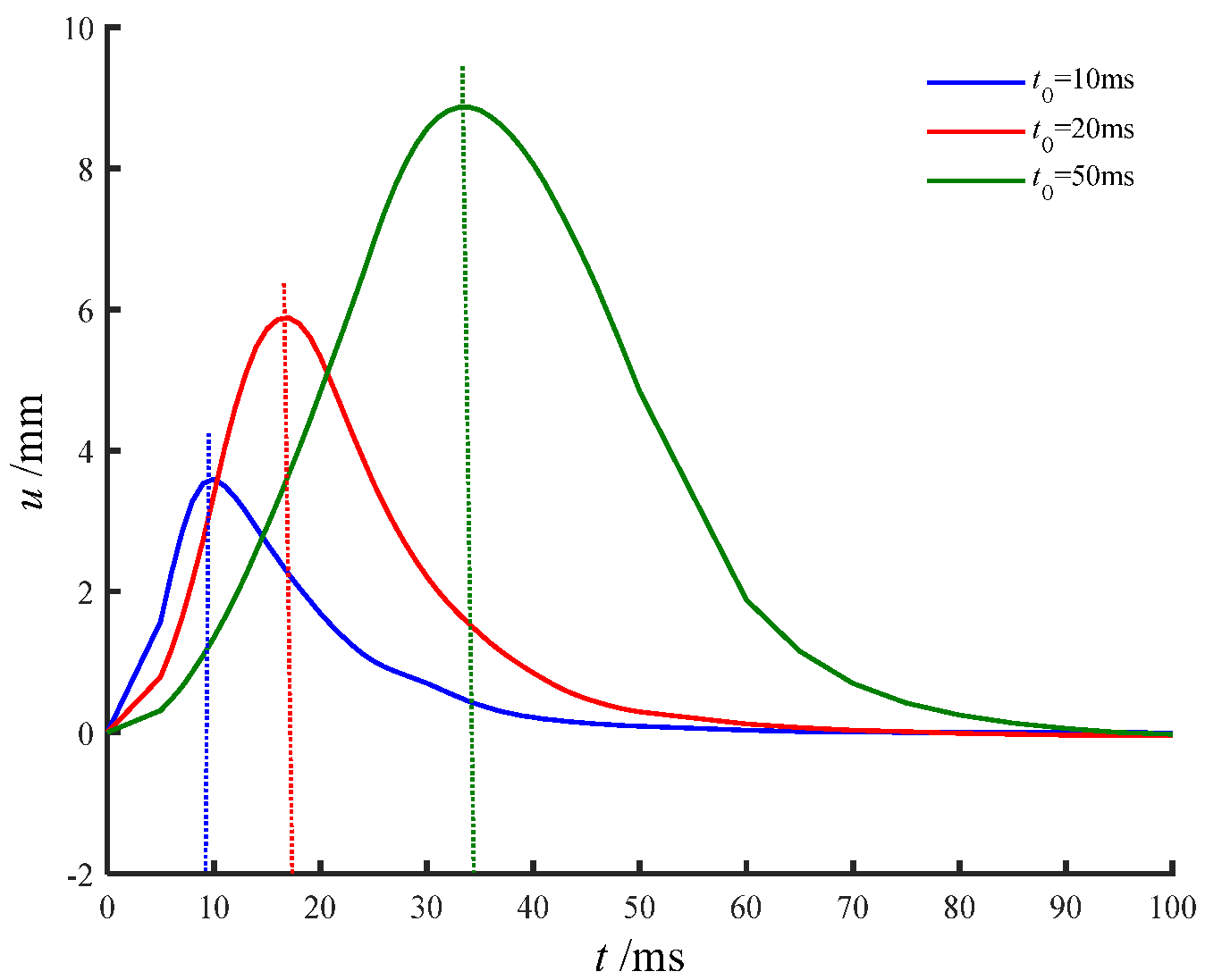
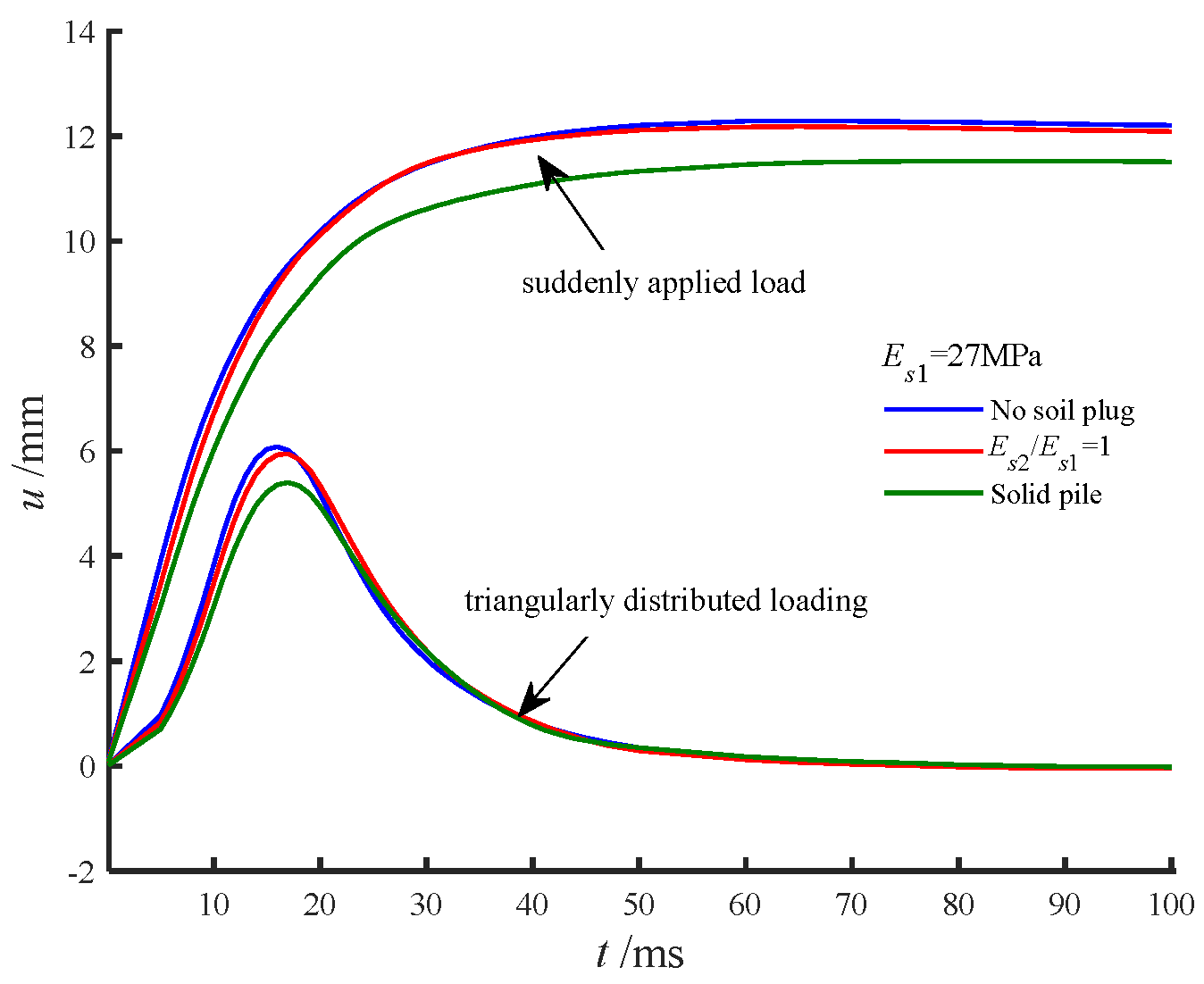
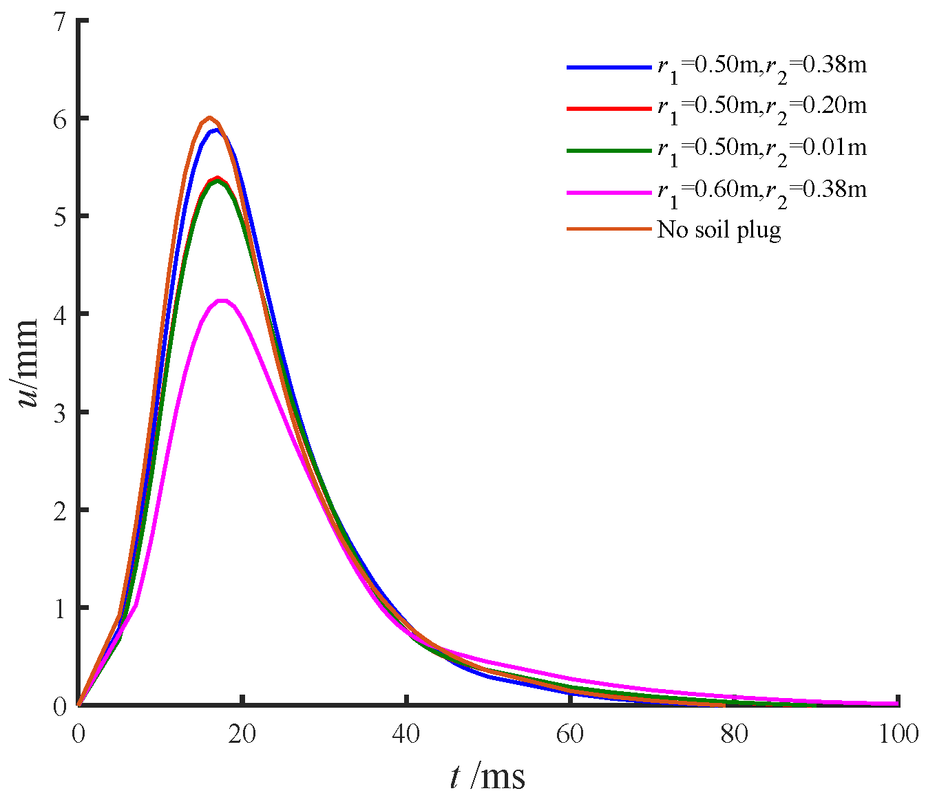
(1)

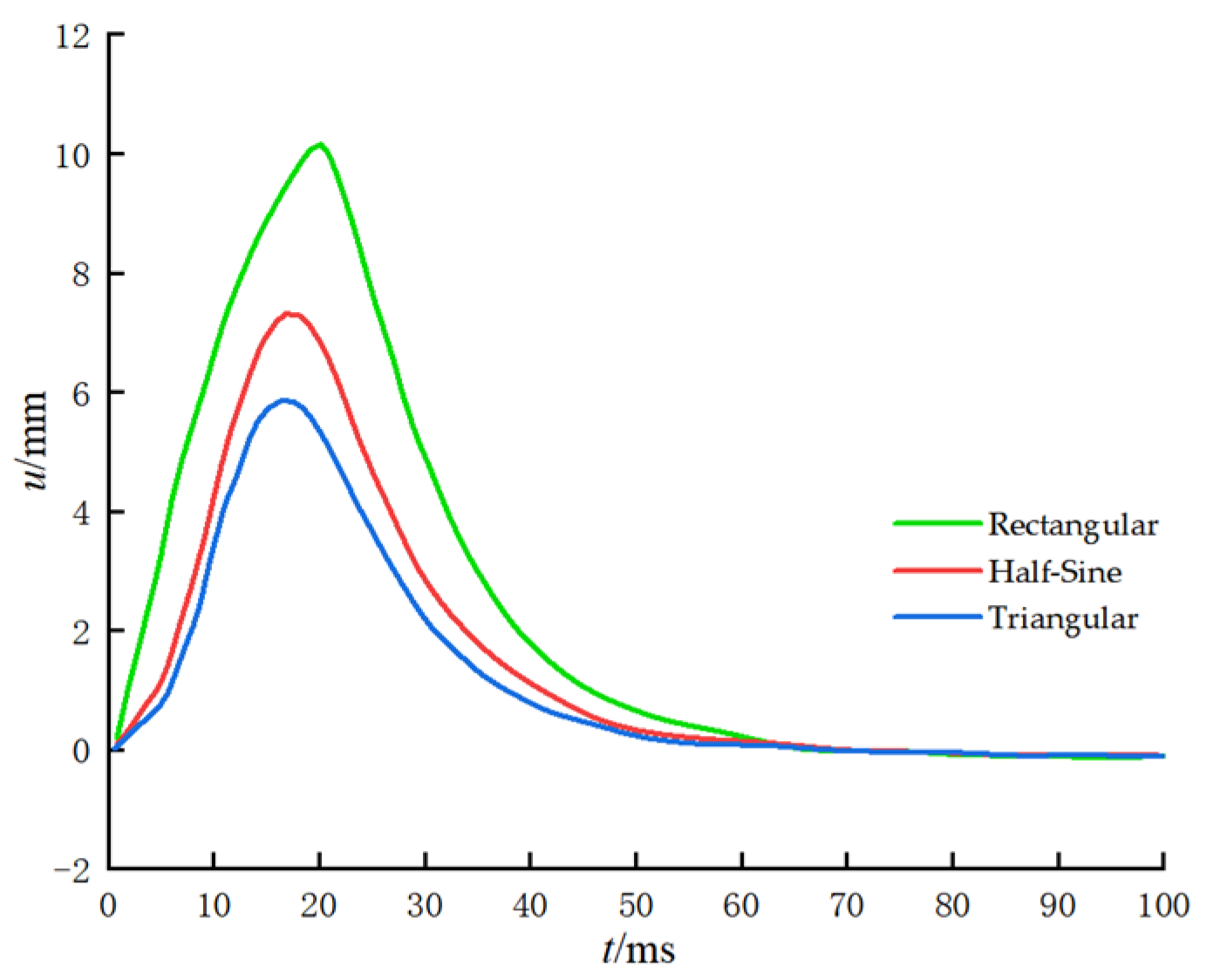
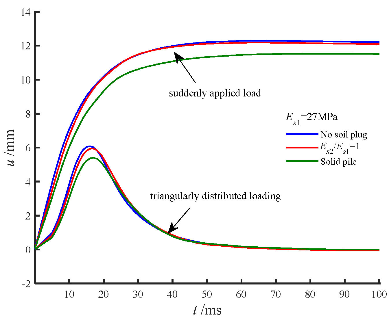
The peak displacement at the pile head increases as the duration of the applied load becomes longer. Core soil inside the tubular pile reduces the peak displacement at the pile head. For piles with small inner diameters, the effect of core soil is minimal and can be ignored, but for larger inner diameters, considering core soil improves the accuracy of the analysis.

(2)

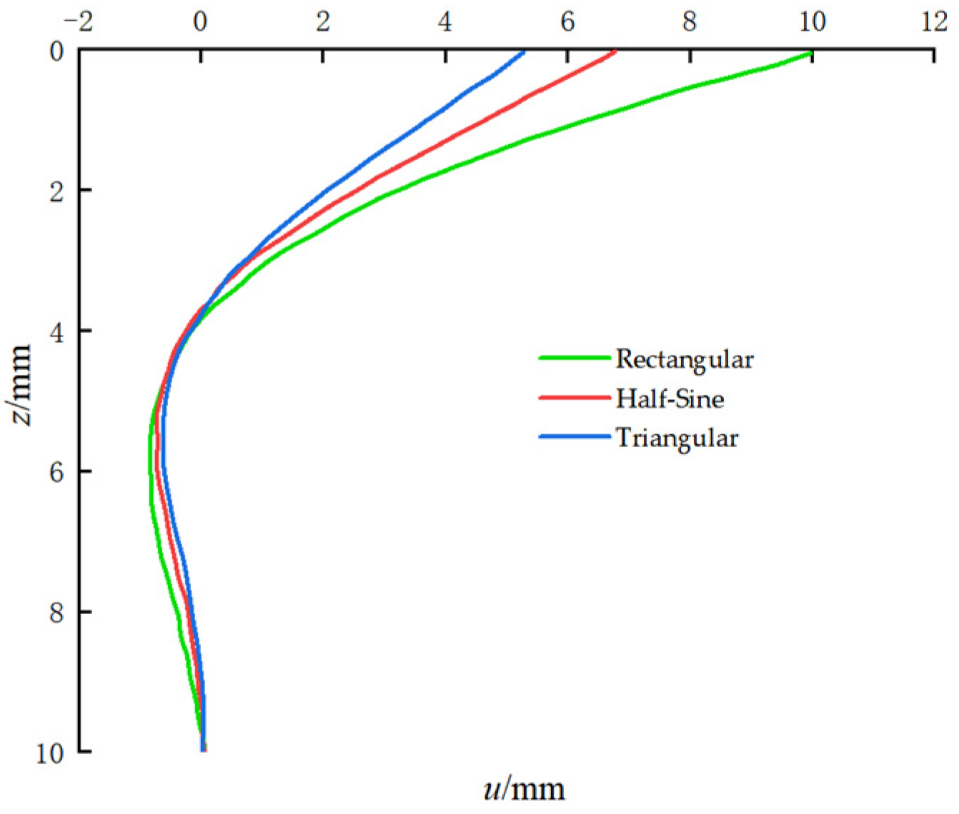
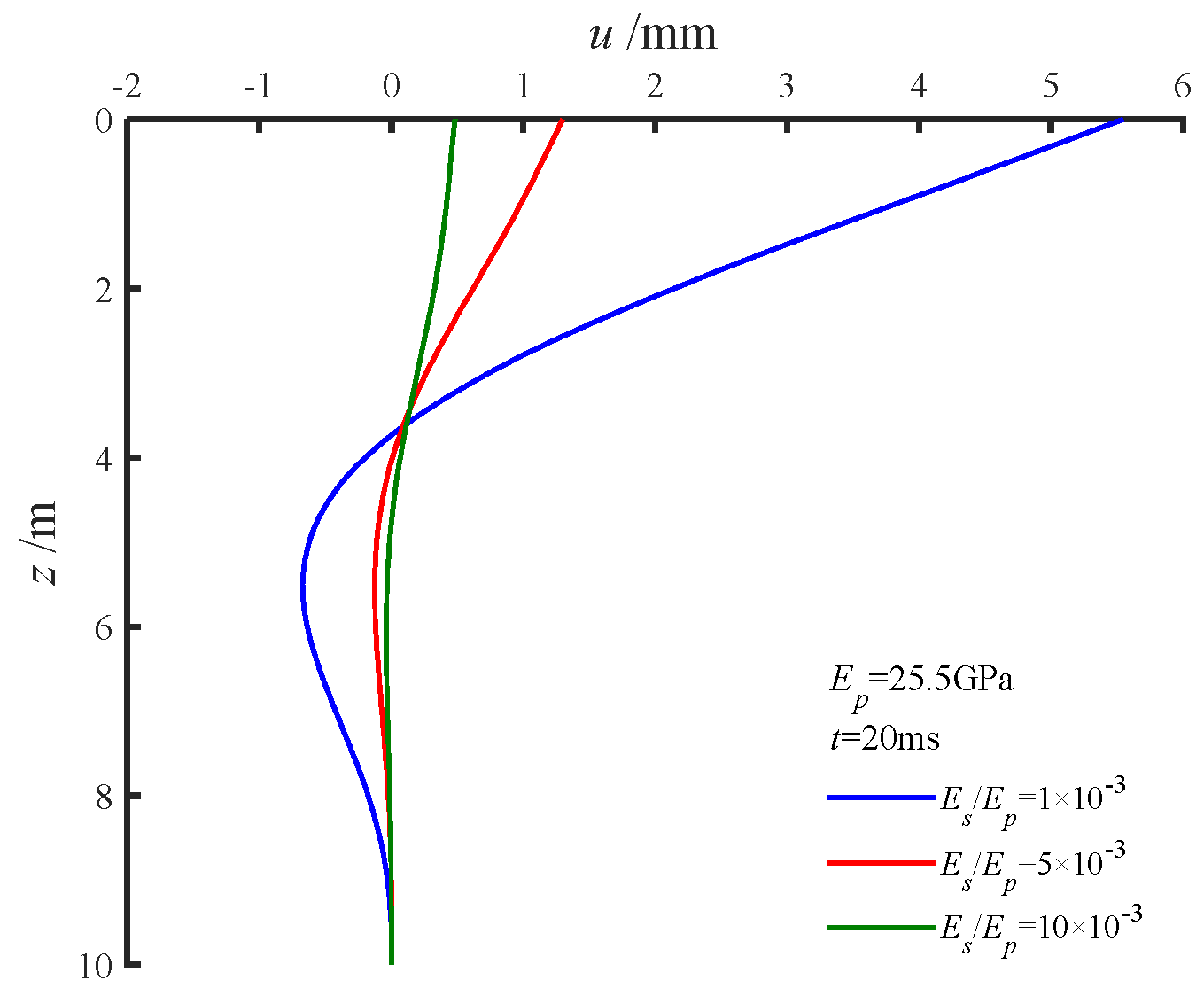
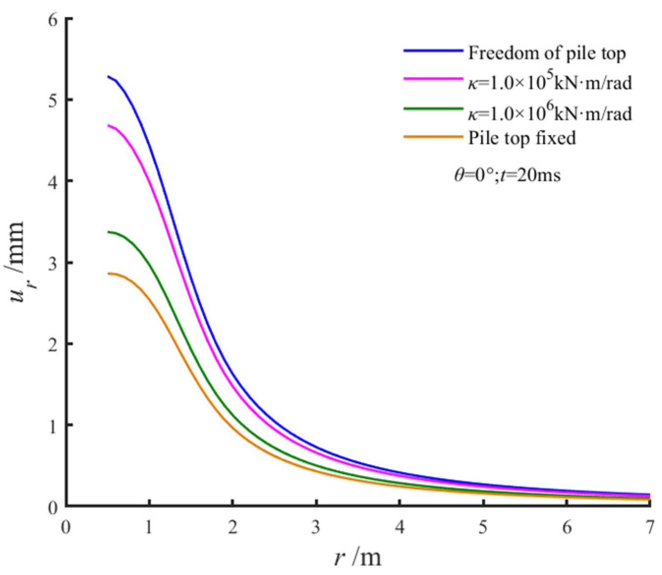
When the pile length exceeds a critical value, known as the effective pile length, the displacement at the pile head stabilizes, and the pile can be treated as infinitely long. Pile displacement decreases rapidly with depth and is significantly reduced by increasing the rotational stiffness at the pile head. Strengthening the pile head constraint effectively enhances the horizontal resistance of the pile.

(3)

The pile head displacement peaks noticeably later than the impact load’s peak force. This lag becomes increasingly significant as the impact duration shortens. Furthermore, the influence of the soil inside the pile on horizontal impact effects is minimal compared to the surrounding soil.

(4)

In both high and low kdi′ regions, the pile head displacement remains nearly constant, forming plateau-like trends. Within the intermediate region, however, displacement increases with kdi′, and the rate of this increase intensifies as soil porosity grows.

(5)

The maximum displacement ratio χ and constraint degree λ are largely invariant in regions of extreme rotational stiffness κ (both high and low). However, within the intermediate flexible constraint range, χ declines steadily with increasing κ.

Our computational model simplifies the analysis of pile–soil interactions but comes with certain limitations. Neglecting soil heterogeneity and anisotropy may reduce the model’s accuracy when applied to layered or stratified soils. Additionally, omitting pile-side friction could underestimate the soil’s restraining effect on the pile, particularly in soft clay or sandy soils.

In future work, we aim to incorporate soil nonlinearity, slippage effects, and pile-side friction into the model to improve its accuracy and broaden its applicability to more complex working conditions.

References

- Rad, M.M.; Ibrahim, S.K. Optimal plastic analysis and design of pile foundations under reliable conditions. Period. Polytech. Civ. Eng. 2021, 65, 761–767. [Google Scholar]
- Rad, M.M. Reliability based analysis and optimum design of laterally loaded piles. Period. Polytech. Civ. Eng. 2017, 61, 491–497. [Google Scholar]
- Zhu, D.; Wang, L.; Wang, Z. Study on pile-soil bonding condition based on transient shock response using piezoceramic sensors. J. Low Freq. Noise Vib. Act. Control. 2024, 43, 358–370. [Google Scholar] [CrossRef]
- Ai, Z.Y.; Wang, X.K.; Ji, W.T. Transient analysis of monopiles embedded in layered saturated soils under vertical excitations. Comput. Geotech. 2023, 155, 105225. [Google Scholar] [CrossRef]
- Li, Y.; Ai, Z.Y. Transient analysis of a fixed-head pile group in multi-layered transversely isotropic media due to horizontal loadings. Comput. Geotech. 2020, 127, 103772. [Google Scholar] [CrossRef]
- Li, Y.; Ai, Z.Y. Horizontal transient response of a pile group partially embedded in multilayered transversely isotropic soils. Acta Geotech. 2021, 16, 335–346. [Google Scholar] [CrossRef]
- Yang, Z.; Zou, X.; Zhou, M.; Huang, L. Effect of the connection mode on the dynamic characteristics of the pile-wheel composite foundation for offshore wind turbines. Comput. Geotech. 2025, 177, 106908. [Google Scholar] [CrossRef]
- Wang, B.; Wang, P.; Zhao, M.; Du, X. Three-dimensional fully coupled analytical solution for a water-pile-saturated soil system under vertical P-wave incident. Appl. Math. Model. 2025, 138, 115825. [Google Scholar] [CrossRef]
- El Naggar, M.H.; Novak, M. Non-linear model for dynamic axial pile response. J. Geotech. Eng. 1994, 120, 308–329. [Google Scholar] [CrossRef]
- El Naggar, M.H.; Novak, M. Nonlinear axial interaction in pile dynamics. J. Geotech. Eng. 1994, 120, 678–696. [Google Scholar] [CrossRef]
- El Naggar, M.H.; Novak, M. Nonlinear lateral interaction in pile dynamics. Soil Dyn. Earthq. Eng. 1995, 14, 141–157. [Google Scholar] [CrossRef]
- Han, Y.C.; Sabin, G.C.W. Impedances for radially inhomogeneous viscoelastic soil media. J. Eng. Mech. 1995, 121, 939–947. [Google Scholar] [CrossRef]
- Han, Y.C. Dynamic vertical response of piles in nonlinear soil. J. Geotech. Geoenviron. Eng. 1997, 123, 710–716. [Google Scholar] [CrossRef]
- Tham, L.G.; Chu, C.K.; Lei, Z.X. Analysis of the transient response of vertically loaded single piles by time-domain BEM. Comput. Geotech. 1996, 19, 117–136. [Google Scholar] [CrossRef]
- Cheung, Y.K.; Tham, L.G.; Lei, Z.X. Transient response of single piles under horizontal excitations. Earthq. Eng. Struct. Dyn. 1995, 24, 1017–1038. [Google Scholar] [CrossRef]
- Nogami, T.; Konagai, K. Time domain axial response of dynamically loaded single piles. J. Eng. Mech. 1986, 112, 1241–1252. [Google Scholar] [CrossRef]
- Novak, M.; Aboul-Ella, F.; Nogami, T. Dynamic soil reactions for plane strain case. J. Eng. Mech. Div. 1978, 104, 953–959. [Google Scholar] [CrossRef]
- Nogami, T.; Konagai, K. Time domain flexural response of dynamically loaded single piles. J. Eng. Mech. 1988, 114, 1512–1525. [Google Scholar] [CrossRef]
- Stacul, S.; Squeglia, N. Simplified assessment of pile-head kinematic demand in layered soil. Soil Dyn. Earthq. Eng. 2020, 130, 105975. [Google Scholar] [CrossRef]
- Mokwa, R.L.; Duncan, J.M. Rotational restraint of pile caps during lateral loading. J. Geotech. Geoenviron. Eng. ASCE 2003, 129, 829–837. [Google Scholar] [CrossRef]
- Catal, H.H. Free vibration of semi-rigid connected and partially embedded piles with the effects of the bending moment, axial and shear force. Eng. Struct. 2006, 28, 1911–1918. [Google Scholar] [CrossRef]
- Sadek, M.; Shahrour, I. Influence of the head and tip connection on the seismic performance of micropiles. Soil Dyn. Earthq. Eng. 2006, 26, 461–468. [Google Scholar] [CrossRef]
- Jiang, L.; Kong, L.; Lin, G.; CHEN, Y. Simplified method of laterally loaded single piles with partial pile head fixity. Eng. Mech. 2014, 31, 63–69. [Google Scholar]
- Yang, Z.; Wu, W.; Liu, H.; Zhang, Y.; Liang, R. Flexible support of a pile embedded in unsaturated soil under Rayleigh waves. Earthq. Eng. Struct. Dyn. 2023, 52, 226–247. [Google Scholar] [CrossRef]
- Li, Y.; Sun, X.; Wu, M. Dynamic response analysis of bridge pier under vehicle collision. Sci. Technol. Eng. 2021, 21, 2471–2478. [Google Scholar]
- Biot, M.A. Theory of propagation of elastic waves in a fluid-saturated porous solid.I. Low-frequency range. J. Acoust. Soc. Am. 1956, 28, 168–178. [Google Scholar] [CrossRef]
- Chen, Y.; Wang, H. Analysis on lateral dynamic response of a pile with the method of reverberation ray matrix. Chin. J. Geotechnocal Eng. 2002, 24, 271–275. [Google Scholar]
- Rong, C.; Hai-Tao, Z.; Song-Tao, X.; He-Sheng, T.; Yuan-Gong, W. Analysis on transverse impact response of an unrestrained Timoshenko beam. Appl. Math. Mech. 2004, 25, 1195–1202. [Google Scholar] [CrossRef]
- Shang, S.; Yu, J.; Wang, H.; Ren, H. Horizontal vibration of piles in saturated soil. Chin. J. Geotech. Eng. 2007, 11, 1696–1702. [Google Scholar]
- Kishi, N.; Chen, W.F.; Goto, Y.; Matsuoka, K.G. Applicability of three-parameter power model to structural analysis of flexibly jointed frames. Mech. Comput. 1991, 20, 238–242. [Google Scholar]
- Ding, X.; Liu, H.; Kong, G.; Zheng, C. Time-domain analysis of velo city waves in a pipe pile due to a transient point load. Comput. Geotech. 2014, 58, 101–116. [Google Scholar] [CrossRef]
- Crump, K.S. Numerical inversion of Laplace transforms using a Fourier series approximation. J. ACM 1976, 23, 89–96. [Google Scholar] [CrossRef]
- Chang, X.M.; Gao, F.; Lu, Z.T.; Long, L.L.; Zhang, J.; Geng, X. A study on lateral transient vibration of large diameter piles considering pile-soil interaction. Soil Dyn. Earthq. Eng. 2016, 90, 211–220. [Google Scholar] [CrossRef]
- Poulos, H.G.; Davis, E.H. Pile Foundation Analysis and Design; Wiley: New York, NY, USA, 1980. [Google Scholar]
Disclaimer/Publisher’s Note: The statements, opinions and data contained in all publications are solely those of the individual author(s) and contributor(s) and not of MDPI and/or the editor(s). MDPI and/or the editor(s) disclaim responsibility for any injury to people or property resulting from any ideas, methods, instructions or products referred to in the content. |
© 2025 by the authors. Licensee MDPI, Basel, Switzerland. This article is an open access article distributed under the terms and conditions of the Creative Commons Attribution (CC BY) license (https://creativecommons.org/licenses/by/4.0/).
Share and Cite
Su, A.; Zhang, M.; Shang, W.; Wang, Q. Transient Horizontal Response of a Pipe Pile in Saturated Soil with a Flexible Support at the Pile Head. Appl. Sci. 2025, 15, 682. https://doi.org/10.3390/app15020682
Su A, Zhang M, Shang W, Wang Q. Transient Horizontal Response of a Pipe Pile in Saturated Soil with a Flexible Support at the Pile Head. Applied Sciences. 2025; 15(2):682. https://doi.org/10.3390/app15020682
Chicago/Turabian StyleSu, Ao, Min Zhang, Wei Shang, and Qiqi Wang. 2025. "Transient Horizontal Response of a Pipe Pile in Saturated Soil with a Flexible Support at the Pile Head" Applied Sciences 15, no. 2: 682. https://doi.org/10.3390/app15020682
APA StyleSu, A., Zhang, M., Shang, W., & Wang, Q. (2025). Transient Horizontal Response of a Pipe Pile in Saturated Soil with a Flexible Support at the Pile Head. Applied Sciences, 15(2), 682. https://doi.org/10.3390/app15020682