Real-Time Optimization of RISC-V Processors Based on Branch Prediction and Division Data Dependency

Abstract

Whether a processor can meet the real-time requirements of a system is a crucial factor affecting the security of real-time systems. Currently, the methods for evaluating hardware real-time performance and the quality of real-time performance are not comprehensive. To address these issues, a “Hardware Real-Time Parameter (H_rtp)” is proposed, which integrates the concepts of “whether it meets real-time system requirements”, “execution speed”, and “operational stability”. This parameter is used to evaluate the real-time performance of RISC-V processors before and after optimization. The processor is optimized for real-time performance using a “simplified local history branch predictor” and a “division data dependency module”. Experimental results show that the processor’s branch prediction accuracy and division calculation speed have both improved. When running the CoreMark benchmark program and the division test program, the test results improved, indicating an enhanced “real-time” performance of the hardware. The changes in the “Standalone Hardware Real-Time Performance Parameter (H_rtp)” data are consistent with theoretical analysis, and it can meet the evaluation needs for “hardware real-time performance”.

1. Introduction

Real-time systems are systems with stringent requirements on operational response time, widely applied in high-safety domains such as aerospace and healthcare [1]. Real-time performance is a critical attribute of real-time systems, directly impacting the overall safety of the system.

There is some debate regarding the concept of real-time systems. Stankovic points out in [2] that real-time systems are those where the computation speed is sufficiently fast. However, Lee argues in [3] that many real-time systems operate on computers with relatively slow processing speeds; therefore, the timing accuracy, predictability, and repeatability of the system are far more important than speed. This perspective is also considered one of the mainstream definitions of real-time performance today. Gong et al. suggest in [4] that real-time performance is relative to the system and represents a requirement for temporal attributes originating from the software application layer.

It is, however, universally acknowledged that within real-time systems, hardware, especially the processor, constitutes a critical substrate for the operation of the entire system. The adequacy of hardware execution time in meeting the real-time constraints imposed by the system is paramount to ensuring the overall safety of the real-time system. The capability of the hardware to fulfill the system’s real-time requirements [5] fundamentally depends on the predictability of its execution time.

There are currently two divergent views on “predictability”. Thiele et al. [6] argue that predictability represents the accuracy of the analysis results concerning the temporal properties of hardware (such as Worst-Case Execution Time, WCET) conducted at the software level (e.g., by compilers). On the other hand, Kirner et al. [7] assert that predictability reflects the variability of actual execution times, with smaller variations indicating better predictability. Irrespective of these perspectives, whether at the level of theoretical analysis or in terms of variations in hardware execution time, the advancement of technologies such as instruction prediction, multi-core architectures, and shared resources [8] has led to increasingly faster processor computational speeds. However, these technological advancements have also resulted in a decrease in the predictability of processor execution times.

Currently, the real-time performance of hardware, particularly processors, primarily manifests in the predictability of their execution times. Mainstream evaluations of hardware predictability still predominantly focus on the system level, encompassing both software and hardware. Specifically, this involves analyzing Worst-Case Execution Time (WCET) results at the software level. This analytical approach, however, has two primary disadvantages.

Firstly, this analytical approach only indicates whether the hardware execution time is predictable, providing a binary outcome of either yes or no. Under the premise that the hardware is predictable, it fails to quantify the degree of predictability, which is essential for evaluating the quality of the hardware’s real-time performance. In other words, while it can determine the presence of predictability, it does not assess the extent to which the predictability is good or poor, thereby limiting the assessment of the hardware’s real-time capabilities.

Secondly, in this evaluation method, the real-time performance assessment of hardware is constrained and limited by the theoretical analysis of software [9]. This situation is particularly pronounced in the development of avionics equipment for civil aviation, where the hardware’s real-time performance must adhere to strict and predefined software requirements. The reliance on software-level analysis can introduce additional constraints and limitations, potentially leading to an incomplete or inaccurate assessment of the hardware’s real-time capabilities.

Therefore, effectively evaluating the predictability (i.e., real-time performance) of hardware processors from a hardware perspective, as well as quantifying the degree of predictability (i.e., the quality of real-time performance), becomes a central focus of this paper.

The contributions of the paper are as follows:

• A parameter is proposed for evaluating the real-time performance and the quality of real-time performance of processors from a hardware perspective, along with the formula for calculating this parameter. This formula not only indicates whether the processor can meet the system’s real-time requirements but also reflects the quality of real-time performance when these requirements are met.
• An embedded RISC-V processor is improved and optimized for real-time performance.
• An improvement in real-time performance is verified, as is the degree of improvement in the quality of real-time performance before and after the processor optimization. Additionally, we use experimental data to validate the reasonableness of the real-time performance parameter.

The paper is organized as follows. Section 2 briefly introduces the current methods for evaluating system real-time performance, such as the WCET method, and discusses its limitations. We also present the real-time performance evaluation method proposed in this paper and provide an explanation. Section 3 introduces the RISC-V processor platform used in this paper and details two specific methods for the real-time optimization of the platform, including the detailed content of module optimizations. Section 4 outlines the phased experiments and results for the optimization of the branch prediction module and the division module. It also describes the comprehensive real-time testing of the complete processor, including the CoreMark test and division test experiments and their results. The section provides an analysis of the overall improvement in the processor’s real-time performance. Section 5 summarizes the WCET analysis method and the H_rtp (Hardware Real-Time Parameter) analysis method, providing experimental conclusions and outlining plans for future work.

2. Related Work

Currently, methods for evaluating the real-time performance of processors (i.e., the predictability of execution time) primarily use embedded [10,11,12,13] real-time systems as the analysis platform. Research methods focusing on the predictability of processor execution time (i.e., real-time performance) mainly concentrate on the analysis of the Worst-Case Execution Time (WCET) of software programs [14]. WCET serves as a critical basis for task real-time scheduling [9], task priority arbitration [15], resource conflict resolution [15], and inter-task communication [11] and is a trusted foundation for ensuring the safe operation of the system [16].

However, the current WCET research approaches have two significant limitations.

Firstly, the worst-case execution paths lack universal representativeness. In actual processor operations, execution paths do not always follow the worst-case execution scenario. This means that WCET alone cannot adequately reflect an objective metric of the processor’s actual hardware performance. As a single metric, WCET fails to capture the predictability of execution time across all possible scenarios.

Secondly, WCET analysis focuses on the execution time under the worst-case path, which represents the maximum execution time [17]. This approach does not provide a comprehensive analysis of the variability in execution time, which is essential for understanding the predictability of the hardware’s execution process.

To better quantify the predictability of hardware execution time (i.e., the real-time performance of the hardware execution process) and the quality of predictability (i.e., the quality of real-time performance), this paper proposes a new parameter, Hardware Real-Time Performance (H_rtp), building upon the existing WCET analysis methods. This parameter aims to provide a more comprehensive and accurate assessment of the processor’s real-time capabilities and the predictability of its execution time.

Integrating the aforementioned concepts, we propose a measurement parameter, H_rtp, to evaluate the “real-time performance” and the “quality of real-time performance” of hardware. The specific calculation formula is as follows in (1) and (2).

$${\mathrm{H}}_{\mathrm{rtp}}{=\mathrm{T}}_{\mathrm{k}}\ln (\mathsf{\mu }+\mathrm{A}\ast {\displaystyle \frac{{\mathsf{\sigma }}^2}{\mathsf{\mu }}})$$

(1)

$${\mathrm{T}}_{\mathrm{k}}=\left\{\begin{array}{l}1\left({\mathrm{T}}_{\mathrm{wcet}}{<\mathrm{T}}_{\mathrm{d}}\right)\\ 0({\mathrm{T}}_{\mathrm{wcet}}\ge {\mathrm{T}}_{\mathrm{d}})\end{array}\right.$$

(2)

In the formula, T_k is used to indicate whether the processor can meet the system’s real-time requirements. T_k is a flag that takes a value of either 1 or 0. A value of 1 indicates that the processor meets the real-time system requirements, while a value of 0 indicates that it does not.

$\ln (\mathsf{\mu }+\mathrm{A}\ast {\displaystyle \frac{{\mathsf{\sigma }}^2}{\mathsf{\mu }}})$ represents the quality of the processor’s execution time (i.e., the quality of its real-time performance) under the condition that the real-time requirements are met. The smaller the value of the parameter, the better the real-time performance of the processor.

μ represents the mean execution time when running specific program instructions, reflecting the “speed” of the processor.

σ² represents the variance in execution time when running specific program instructions, indicating the “stability” of the processor.

By considering both μ and σ², the assessment of “hardware (processor) real-time performance” becomes more accurate and comprehensive, taking into account both the speed and the variability of the processor’s operation.

A is a weighting constant that ranges between 0 and 100. Users can adjust A based on their specific requirements to balance the importance of “execution speed” and “stability”. For example, in a real-time system where the stability of the processor’s operation is significantly more important than its speed, the value of A can be set to the maximum, 100. Conversely, if the speed of the processor is much more critical than its stability, the value of A can be set to 1. This flexibility allows users to tailor the assessment to their specific needs.

T_wcet represents the worst-case execution time (WCET) of the hardware when executing a specific segment of program instructions. There are various methods for calculating this parameter, which are not extensively discussed in this paper. For detailed information, please refer to [18,19,20], etc.

T_d represents the real-time constraint time allocated to the processor by the real-time system. This parameter is distributed by the real-time system and is not extensively discussed in the paper. When T_wcet is less than T_d, it indicates that the processor meets the system’s real-time requirements during the execution of a specific computation, and T_k is set to 1. Otherwise, T_k is set to 0.

When H_rtp = 0, it signifies that the processor fails to meet the real-time requirements specified by the real-time system.

In cases where H_rtp ≠ 0, a smaller value of H_rtp indicates that the processor, while satisfying the system’s real-time requirements, exhibits superior execution speed and stability, thereby demonstrating enhanced real-time performance. Conversely, a larger value of H_rtp suggests inferior real-time performance.

In addition to the above statements, some further clarifications regarding H_rtp are as follows:

• The hardware real-time performance parameter (H_rtp) does not conflict with the real-time performance of computer systems (or embedded systems) mentioned earlier. H_rtp is an extension of the foundational concept of system real-time performance and does not negate or invalidate the existing concept of real-time performance in computer systems (or embedded systems).
• Depending on the specific program executed by the processor, the independent hardware real-time performance parameter H_rtp can have multiple sub-cases. For example, there can be a parameter H_{rtp_taskA} corresponding to the execution of Task A and a parameter H_{rtp_coremark} corresponding to the execution of the CoreMark benchmark program.
• The input parameters μ and σ² for H_rtp are statistical data obtained from the actual operation of the processor. The sample size is determined based on the processor’s application context, typically using large sample sizes (generally greater than 80).
• This paper does not directly use σ² to evaluate the real-time performance of the processor because σ² is a qualitative measure of stability rather than a quantitative one.
  For example, consider an extreme case where two processors execute the same program segment:
  Processor A: μ = 5 s, σ² = 3 s; Processor B: μ = 50 s, σ² = 5 s.
  If we simply compare σ², Processor A appears to have better stability because 3 s < 5 s.
  However, when considering the variability as a percentage of the mean, observe the following:
  Processor A: Variability = 3/5 × 100% = 60%; Processor B: Variability = 5/50 × 100% = 10%.
  From this perspective, Processor B clearly demonstrates better stability. This approach to analysis is more reasonable and provides a more accurate assessment of the processor’s real-time performance.

3. Optimization of Real-Time Performance for RISC-V Processors

3.1. RISC-V Processor Platform

The RISC-V instruction set is an open-source and free instruction set architecture (ISA) that offers several advantages, including simplicity, adaptability, customizability, and the absence of conditional code and branch delay slots [21]. These advantages allow users to flexibly customize and optimize the ISA according to the specific requirements of their applications.

The RISC-V processor prototype used in this paper is derived from the open-source project Tinyriscv and utilizes the RV32IM instruction set. After expanding the modules of Tinyriscv, it is named Rev-riscv. Rev-riscv employs a three-stage pipeline structure, and the detailed architecture of the processor is shown in Figure 1.

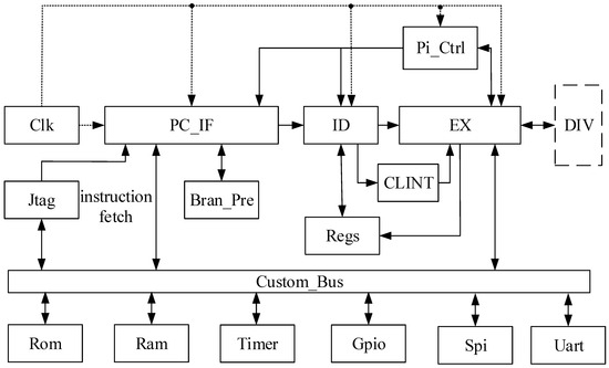
Figure 1. Rev-riscv processor architecture diagram.

The three-stage pipeline operates as follows: fetch, decode, and execute. In the first stage (PC_IF module), the next instruction address to be fetched is calculated, and the instruction is then retrieved from the instruction memory (Rom module) via the bus (Custom_Bus module). In the second stage (ID module), the instruction is decoded, and the corresponding data are fetched from the register file (Regs module). In the third stage (EX module), the operations specified by the instruction, such as arithmetic and logic calculations, write-back, jumps, and halts, are performed. The remaining modules are used for data processing, pipeline control, and other functions within the processor. The descriptions of the various modules are shown in Table 1.

Table 1. Introduction to the various modules of Rev-riscv.

Module Name	Description
Clk	Provides the clock signal for the processor’s operation.
PC_IF	Calculates and retrieves the Program Counter value.
ID	Decodes the instructions.
EX	Performs data operations and instruction execution.
Pi_ctrl	Responsible for controlling the pause and resumption of the pipeline.
DIV	Performs division operations.
Jtag	Used for circuit testing and debugging.
Bran_Pre	Predicts the outcomes of conditional branch instructions.
CLINT	Arbitrates interrupt signals.
Regs	Stores general-purpose register data.
Custom_Bus	Connects the CPU to peripheral modules.
Rom	Stores the instruction information corresponding to the software.
Ram	Stores the data information corresponding to the software.
Timer	Performs timing and generates timer interrupts.
Gpio	Provides basic input/output functionality.
Spi	Connects SPI interface devices.
Uart	Executes serial data transmission and reception.

3.2. Optimization of the Bran_Pre Module (Branch Prediction Module)

3.2.1. Introduction to Branch Jump Instructions

In a three-stage pipeline processor, the execution stage is the third stage. When the execution stage resolves the correct target address of a branch, if the instructions in the first two stages of the pipeline are not the instructions at the target address, the pipeline needs to be flushed. Therefore, when the processor executes a conditional branch, a correct prediction of a single instruction saves two clock cycles compared to an incorrect prediction.

We will use a specific set of instructions corresponding to a program segment to explain this. In Figure 2, the instruction at PC address “32’h00000038” is a jump instruction (32’hfec5e8e3), which specifies a jump to the instruction at PC address “32’h00000028”.

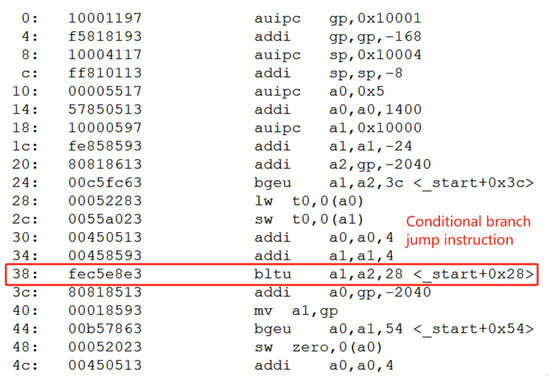
Figure 2. Conditional branch jump instruction in disassembled code.

In Figure 3, the processor makes an incorrect prediction and does not perform the jump. It only determines the correct jump address and direction in the third stage, thus incurring an additional two clock cycles. This results in the processing of two incorrect instructions.

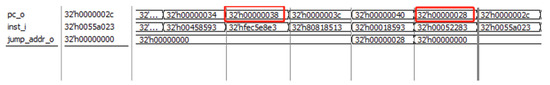
Figure 3. The figure of pc_o values (instruction addresses) in the case of an incorrect prediction.

In Figure 4, the branch predictor correctly anticipates the jump result and the target address, so the PC value directly jumps to 32’h00000028. Compared to the scenario in Figure 3 where the prediction was incorrect, this saves two clock cycles.

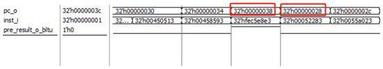
Figure 4. The figure of pc_o values (instruction addresses) in the case of a correct prediction.

We use compilation tools such as Eclipse to compile test programs like CoreMark. In the generated execution instructions, conditional branch instructions account for approximately 20% of the total instructions (detailed data are shown in Figure 5). If all conditional branch predictions are correct, it can save about 10% of the processor’s execution time. Therefore, adding a branch prediction module can significantly improve the processor’s execution speed.

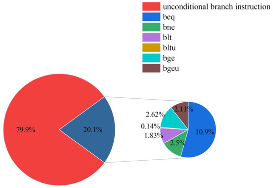
Figure 5. The proportion of conditional branch instructions to unconditional branch instructions.

The Rev-riscv processor supports six conditional branch instructions: beq, bne, blt, bltu, bge, and bgeu. The detailed explanations of each instruction are provided in Table 2.

Table 2. Conditional branch instructions and descriptions.

Instruction	Description
beq	Branch if equal: Jumps to the target address if the values in the two specified registers are equal.
bne	Branch if not equal: Jumps to the target address if the values in the two specified registers are not equal.
blt	Branch if less than: Jumps to the target address if the value in the first specified register is less than the value in the second specified register (signed comparison).
bltu	Branch if less than unsigned: Jumps to the target address if the value in the first specified register is less than the value in the second specified register (unsigned comparison).
bge	Branch if greater than or equal: Jumps to the target address if the value in the first specified register is greater than or equal to the value in the second specified register (signed comparison).
bgeu	Branch if greater than or equal unsigned: Jumps to the target address if the value in the first specified register is greater than or equal to the value in the second specified register (unsigned comparison).

The proportions of the six conditional branch instructions among all conditional branch instructions are shown in Figure 5.

Therefore, how to improve the prediction success rate of conditional branch instructions and reduce the processor’s runtime has become a focus of this paper.

3.2.2. Optimization of the Branch Predictor

One method to improve the prediction accuracy of conditional branch instructions is to optimize the branch prediction module of the processor.

The branch prediction module in Rev-riscv uses a static branch predictor. It is configured such that if the instruction jumps backward (i.e., the target PC value is greater than the PC value of the branch instruction), it always predicts that the jump will be taken. Otherwise, it predicts that the jump will not be taken.

The accuracy of static branch prediction is around 60% [22]. To improve the success rate of branch prediction and enhance the overall execution speed and stability of the processor, this paper designs a simplified local branch history predictor (SLBHP) to optimize the branch prediction component of the Rev-riscv processor.

The simplified local branch history predictor is an optimized version of the local branch history predictor. In a conventional local branch history predictor [23], the main components are the Branch History Register (BHR), the Branch Target Buffer (BTB), and the Pattern History Table (PHT). The Branch History Register (BHR) stores the historical prediction data for individual branch instructions. The typical structure of a branch history predictor is shown in Figure 6.

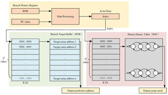
Figure 6. Traditional local branch history predictor principle diagram.

For embedded systems, a branch history predictor consumes relatively large resources. It typically includes 2^k index registers, 2^k Branch Target Buffers (BTB), and 2^k Pattern History Tables (PHTs). Given the limited resources of embedded processors, a branch history predictor is not an ideal choice for branch prediction.

We adopt a simplified local branch history predictor (SLBHP) to perform branch prediction for the current processor. The simplified local branch history predictor (SLBHP) is an optimized version of the traditional local branch history predictor. The main optimizations include omitting the Branch Target Buffer (BTB) structure, directly indexing instructions with the index variable without evaluating the 32-bit PC value, and reducing the index size from k bits to 4 bits. The optimized simplified branch history predictor is shown in Figure 7.

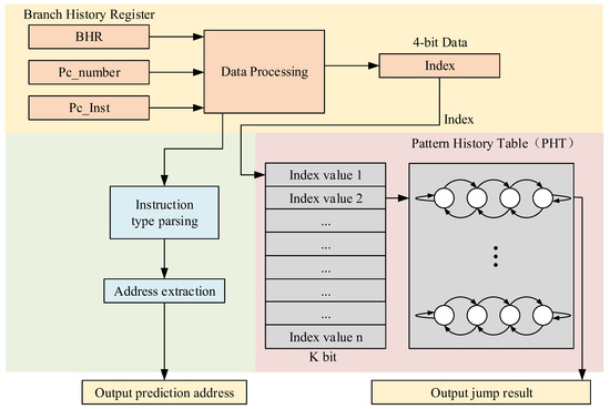
Figure 7. Simplified local branch history predictor (SLBHP) principle diagram.

The streamlined branch history predictor’s internal prediction function workflow is as follows:

(1)

Receive the “PC_inst” signal and “PC_number” signal from the fetch stage. The BHR signal is an internal update signal for the SLBHP (simple loop branch history predictor).

(2)

Evaluate the “PC_inst” signal; if it is a branch instruction, extract the target address and prepare to output the branch address (prediction address).

(3)

Based on the “PC_number” and the instruction type obtained through “PC_inst”, index the “Index” value in the BHR.

(4)

Use the “Index” value to access the corresponding 2-bit saturating counter in the PHT (Pattern History Table).

(5)

Output the branch result (prediction result) based on the state of the indexed 2-bit saturating counter.

The simplified branch history predictor module operates in the first stage of the pipeline (fetch stage). It primarily uses combinational logic design, which does not consume additional clock cycles. The input and output signals of this module are shown in Table 3.

Table 3. Signals related to the simplified branch predictor.

Instruction Name	Input/ Output	Description
PC_inst	Input	The instruction from the PC_IF (fetch) module.
PC_number	Input	The PC value of the instruction from PC_IF module.
Ex_jump_valid	Input	The true branch result from the EX (execution) module.
EX_inst	Input	The instruction from the EX (execution) module.
To_CTRL_not_flash	Output	The pipeline flush signal output to the Pi_Ctrl module.
To_PC_If	Output	The predicted PC value output to the PC_IF module.

The workflow for SLBHP (simplified local branch history predictor) to update the BHR status and interact with external signals is as follows:

(1)

Based on the input “PC_inst” signal and “PC_number”, along with the state of the PHT (Pattern History Table), the SLBHP first predicts the branch and outputs the prediction result to the “PC_generate” module, which is used to generate subsequent PC values (SLBHP Prediction Workflow).

(2)

The SLBHP updates the BHR records within it based on the actual executed instructions and the actual calculated branch flag signals provided by the subsequent “EX” (Execution) module.

(3)

The actual calculated branch flag signal and the branch outcome from the corresponding 2-bit saturating counter are used to determine if the prediction was correct. If the prediction was accurate, no pipeline flush occurs, and the saturating counter state shifts towards a stronger branch direction. If the prediction was incorrect, the saturating counter state shifts towards a weaker branch direction, and a pipeline flush signal is sent to the “Pi_Ctrl” (pipeline control) module to flush the pipeline and refetch instructions from the target address for execution.

The principle diagram of the branch prediction module is shown in Figure 8.

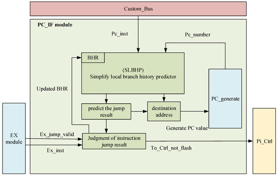Figure 8. Branch predictor module working principle diagram.

3.3. Optimization of the DIV Module (Division Module) Based on Data Dependency

3.3.1. Division Module and Its Working Principle

In the Rev-riscv, the divider uses the trial division method, which requires 33 clock cycles for each division operation. During these 33 clock cycles, the pipeline is paused. This approach limits the processor’s operating speed.

When performing a division operation, the divider outputs a busy (in calculation) flag signal to the Ex (execute) module. The Ex (execute) module then converts this signal into a pipeline pause signal, thereby suspending the entire processor’s pipeline process.

The trial division method works by shifting and comparing the dividend (or the intermediate value of the dividend minus the divisor) with the divisor. The comparison result (1 or 0) is used as the corresponding bit value of the quotient. The schematic diagram of the divider is shown in Figure 9.

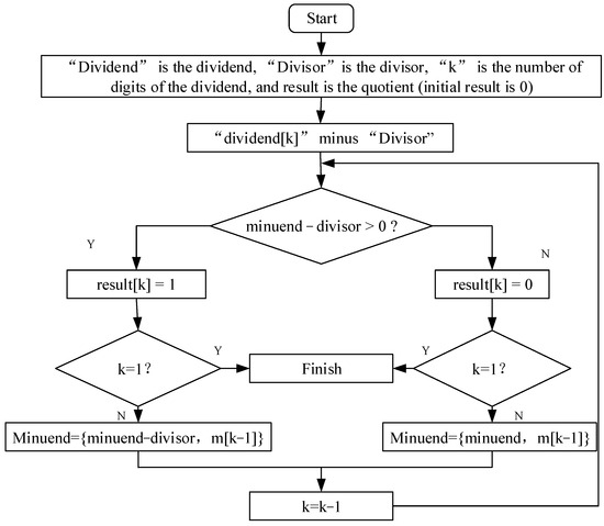
Figure 9. Divider working principle diagram.

3.3.2. Division Instruction Data Dependency Judgment and Optimization

To improve the execution efficiency of division operations in the processor, we adopt two methods to enhance the performance of the divider.

First, increase the driving clock of the divider from 50 M to 300 M to speed up the divider.

Second, add a data dependency judgment module. If the subsequent instructions do not use the result of the division, the pipeline will not be paused, thereby improving the execution speed.

The data dependency judgment module is designed to evaluate the data relationship between division instructions and subsequent instructions. Therefore, the data dependency judgment logic is placed in the Id (decode) stage of the pipeline, which is the stage before the Ex (execute) stage. The optimized data dependency module, located in the Id (decode) stage, outputs corresponding signals to the pipeline control module (Pi_Ctrl) based on the results of the data dependency judgment. The signals in the Id (decode) module that involve data dependencies are shown in Table 4.

Table 4. Introduction to signals of the division dependency module.

Signal Name	Input/ Output	Description
Div_busy_i	Input	The signal indicating that a division operation is in progress.
Div_reg_waddr	Input	The address to which the division result is written.
PC_inst	Input	The instructions following the division instruction.
Div_hold_flag	Output	The pipeline stall signal corresponding to the division calculation.

The flowchart for the data dependency judgment of division operations is shown in Figure 10.

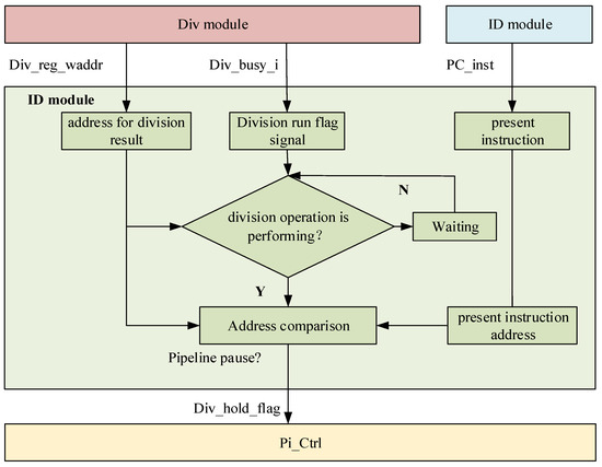
Figure 10. Division data dependency module working principle diagram.

During the division calculation, the “Div_busy_i” signal remains high (1), and the “Div_reg_waddr” signal provides the write address for the division result. When the subsequent instruction (PC_inst) is decoded, it decodes the data address of that instruction. If the data address of the subsequent instruction (PC_inst) matches the write address of the division result, the pipeline is paused to wait for the completion of the division operation. Otherwise, the pipeline is not paused.

4. Experiment and Result Analysis

4.1. Experimental Preparation

We implemented the Rev-riscv processor using Verilog code. Building on this foundation, we developed the Rev-riscv-II processor platform with an optimized branch prediction module and added data dependency judgment. For running smaller-scale programs to save time, we used ModelSim SE-64 10.5 (Mentor Graphics, Wilsonville, OR, USA) for simulation. The EDA development tool Vivado HLS 2018.3 (Xilinx, San Jose, CA, USA) was utilized to verify and conduct practical testing of both the pre-optimized and optimized processor platforms, as well as to evaluate resource consumption before and after design optimization. Both processors were successfully run on the ARTIX-7 series FPGA (XC7A100T, EmbedFire, Dongguan, China). We used the officially provided RISC-V compilation tool Eclipse (Eclipse Foundation, Ottawa, ON, Canada) to generate assembly files corresponding to C-language test programs (in RISC-V assembly language) and then used the Opcode tool (Windows Power Shell, Microsoft, Redmond, WA, USA) to download the compiled files to the FPGA.

Since the CoreMark benchmark program is a widely accepted industry standard for processor benchmarking, we use CoreMark to test the overall real-time performance of the processor. Additionally, because the division tests in CoreMark account for only a small proportion, while conditional branch prediction instructions have a normal presence, we have supplemented with a self-test case for division to evaluate the real-time performance of the processor when running high-density division instructions. (Branch prediction is sufficiently tested within the CoreMark tests, so no additional test cases were added specifically for this purpose).

The distribution of this subsection is as follows:

First, phased experiments are conducted to verify the optimization results of branch prediction and division data dependency.

Then, the CoreMark test cases and division test cases are used to validate the overall improvement in the real-time performance of the processor.

Finally, a summary and analysis of the real-time test results are provided.

4.2. Stage Experiments and Result Analysis

We conducted multiple comparative experiments on the processor before and after optimization. We used the CoreMark benchmark program to test the prediction accuracy of branch prediction instructions and the division calculation speed when executing division operation instructions.

4.2.1. Branch Prediction Test Results and Analysis

We implemented two types of branch predictors using Verilog code: the simplified branch history predictor (SLBHP) and the static branch predictor. Both branch predictors were integrated into the Rev-riscv processor. We used Vivado to analyze the resource consumption in both scenarios, as shown in Table 5.

Table 5. Comparison of the main resource consumption of two branch predictors.

Resource Name	Processor with Static Branch Predictor	Processor with Simplified Local Branch History Predictor (SLBHP)
LUT	11,203	13,926
LUTRAM	4200	4216
FF	6211	6410

The simplified branch history predictor (SLBHP) increases the overall resource consumption (LUTs) of the processor by 24% (2723 units) compared to the static branch predictor.

In the hardware design code, to better monitor the number of jump instructions executed and the number of correct predictions, we have added a jump count register (Skp_counter) to display the number of executed jump instructions. Additionally, we have incorporated a correct jump prediction count register (Skp_right_counter) to show the number of times predictions were accurate. We use the Logic Analyzer (ILA) provided by Vivado to observe the values of these two counters for data collection. A screenshot of the data capture at a particular instance is shown in Figure 11.

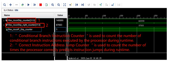
Figure 11. A screenshot of the analysis from the embedded Logic Analyzer (ILA).

The data were calculated and analyzed, with the prediction accuracy of the static branch predictor shown in Table 6. The prediction accuracy of the simplified local history branch predictor is shown in Table 7.

Table 6. Accuracy of the static branch predictor.

Serial Number	Number of Branch Instructions	Number of Correct Branches	Prediction Accuracy	Average Accuracy
1	140,890	88,338	62.7%	61.3%
2	140,293	87,683	62.5%
3	140,594	89,277	63.5%
4	141,122	87,072	61.7%
5	140,951	90,631	64.3%
6	140,584	89,833	63.9%
7	140,964	87,116	61.8%
8	140,458	89,612	63.8%
9	140,367	89,414	63.7%
10	140,485	88,646	63.1%

Table 7. Accuracy of the simplified branch history predictor (SLBHP).

Serial Number	Number of Branch Instructions	Number of Correct Branches	Prediction Accuracy	Average Accuracy
1	140,791	103,904	73.8%	73.96%
2	140,489	101,714	72.4%
3	140,852	105,076	74.6%
4	140,981	101,365	71.9%
5	141,254	102,409	72.5%
6	141,685	108,956	76.9%
7	140,756	104,441	74.2%
8	140,951	103,458	73.4%
9	140,501	105,797	75.3%
10	140,684	104,950	74.6%

The simplified branch history predictor (SLBHP) can improve the prediction accuracy of the Rev-riscv processor by approximately 10% compared to the static branch predictor.

In summary, the simplified branch history predictor can increase the branch prediction accuracy of the processor by about 12% compared to the static branch predictor at the cost of consuming approximately 24% (2723 units) more LUT resources. The total LUT resources of the FPGA development board with model XC7A100T are 53,200. A resource consumption of 2723 units is within an acceptable range.

4.2.2. Division Instruction Simulation and Analysis

We implemented the data dependency judgment module for division operations using Verilog code and integrated it into the Rev-riscv processor. The implementation was performed on an FPGA, and we used Vivado to observe the resource consumption before and after the addition of the module. The resource consumption is shown in Table 8.

Table 8. Resource overhead of processors equipped with different branch predictors.

Resource Name	Processor with Static Branch Predictor	Processor with Simplified Local Branch History Predictor (SLBHP)
LUT	13,926	15,161
LUTRAM	4216	4241
FF	6410	6428

We used ModelSim to perform simulation tests on the processor with the added division data dependency module. Before the optimization of the division module, a single division operation required 33 clock cycles, during which the PC value was paused for 30 clock cycles, as shown in Figure 12.

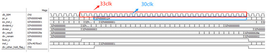
Figure 12. Original divider module function simulation diagram.

After optimizing the division data dependency, in the least ideal conditions, a single division operation consumes six clock cycles at 50 M, as shown in Figure 13.

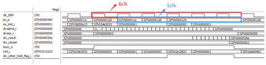
Figure 13. Optimized divider module function simulation diagram.

Under the most ideal conditions, division calculations no longer require the pipeline to pause.

By optimizing the processor for data dependencies, the time required for division operations can be reduced from 33 clock cycles to 6 clock cycles, with the PC value needing to pause for only 5 clock cycles. Under the most ideal conditions, division calculations no longer require the pipeline to stall. The reduction in the time required for division calculations exceeds 75%.

In summary, by adding the division data dependency module, the overall resource usage increases by approximately 9.1%, while the division calculation time is reduced by more than 75%.

4.3. Processor Real-Time Testing and Performance Analysis

This section primarily focuses on the implementation of two RISC-V processors, Rev-riscv and Rev-riscv-II, on an FPGA for subsequent testing.

To make the verification process more practically relevant, this paper assumes a research background in automotive autonomous driving systems (real-time systems). The relationship between the real-time system and the processors is illustrated in Figure 14.

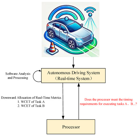
Figure 14. Diagram of the Interaction between autonomous driving real-time system and processor.

The real-time system plans to use three processor models for the autonomous driving system: Rev-riscv, Rev-riscv-II, and Rev-riscv-III (the latter has not been implemented and is included only as a negative reference).

In this real-time system, the processors primarily execute the following two types of computational tasks:

(1)

Conventional performance computations (primarily based on test contents from CoreMark such as matrix operations and list processing) used for routine information processing.

(2)

High-density multiplication operations used to calculate information such as the current vehicle speed.

Failure to provide results for these two types of computations within the specified time limits of the real-time system can lead to severe consequences, including car accidents.

After data analysis by the real-time system software, the following requirements are specified:

(1)

The processor must complete Task A (CoreMark tests) within 100 s (denoted as T_d in the formula) to meet system requirements and avoid hazardous outcomes.

(2)

The processor must complete Task B (performing 200 division operations) within 100 microseconds (also denoted as T_d in the formula) to meet system requirements and avoid hazardous outcomes.

The workflow relationship between tasks is shown in Figure 14. The metric information for Task A and Task B is provided in Table 9.

Table 9. Descriptions and maximum execution deadlines for Task A and Task B.

Task Name	Task Content	System-Required Maximum Execution Time (Td)
Task A	CoreMark Performance Test	100 s
Task B	Division Operation Test	300 µs

4.3.1. CoreMark Overall Performance Testing and Comparative Analysis

The H_rtp parameter calculation formulas are shown in (1) and (2).

In the formula, T_k is the indicator of whether the hardware meets the system’s real-time requirements. T_d (the data corresponding to Task in Table 9) is generally provided by the real-time system. T_wcet refers to the Worst-Case Execution Time (WCET) of the processor when running Task A, which can be determined through various analysis methods. Since the calculation of T_wcet is not the focus of this paper, we directly provide assumed WCET values for the three processors, as shown in Table 10.

Table 10. The processor’s WCET and the system-required maximum task execution time for Task A.

Processor Name	Twcet of Processor for Task A	The System-Specified Td for Task A
Rev-riscv	90 s	100 s
Rev-riscv-II	90 s
Rev-riscv-III	110 s

First, analyze the H_rtp of the Rev-riscv-III processor. Since T_wcet > T_d, this indicates that in this case, T_k = 0 and H_rtp = 0; the processor cannot meet the real-time metrics allocated by the real-time system, making it unsuitable for this real-time system.

For the other two processors, T_wcet < T_d, and T_k = 1; therefore, a detailed calculation of H_rtp can be performed to evaluate the real-time performance metrics of Rev-riscv and Rev-riscv-II under these conditions.

Assuming that the real-time system places high importance on fluctuations in processor execution time, the value of A is set to 100 under these conditions. The H_rtp parameter calculation formulas are revised as shown in (3) and (4).

$${\mathrm{H}}_{\mathrm{rtp}}{=\mathrm{T}}_{\mathrm{k}}\ln (\mathsf{\mu }+100\ast {\displaystyle \frac{{\mathsf{\sigma }}^2}{\mathsf{\mu }}})$$

(3)

$${\mathrm{T}}_{\mathrm{k}}=\left\{\begin{array}{l}1({\mathrm{T}}_{\mathrm{w}\mathrm{c}\mathrm{e}\mathrm{t}}<{\mathrm{T}}_{\mathrm{d}})\\ 0({\mathrm{T}}_{\mathrm{w}\mathrm{c}\mathrm{e}\mathrm{t}}\ge {\mathrm{T}}_{\mathrm{d}})\end{array}\right.$$

(4)

The CoreMark benchmark scores were obtained for the unoptimized Rev-riscv processor and the Rev-riscv-II processor, which has been optimized for branch prediction and division data dependency. Each processor was run 100 times, and the data before and after optimization were compared. The detailed runtime data are shown in Table 11.

Table 11. Test data for Rev-riscv and Rev-riscv-II when running the CoreMark benchmark program.

Test Item	Rev-Riscv	Rev-Riscv-II
Number of Tests	100	100
Mean Runtime	77.7191 s	74.0996 s
Variance of Runtime	3.47505	2.85681
Hrtp Value	4.4091	4.3578

The score time–frequency distribution of the Rev-riscv processor is shown in Figure 15a. The score time–frequency distribution of the Rev-riscv-II processor is shown in Figure 15b. From the qualitative analysis of the data distribution, the μ (mean) and σ (standard deviation) of Rev-riscv-II are slightly better than those of Rev-riscv, which roughly suggests that the real-time performance of Rev-riscv-II is slightly better than that of Rev-riscv.

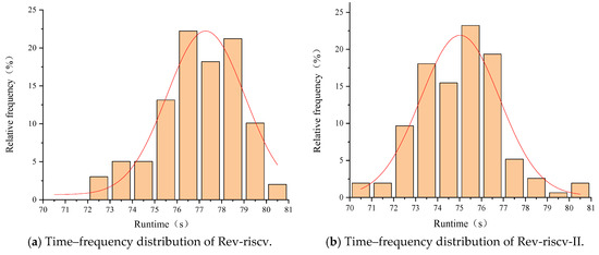
Figure 15. Time–frequency distribution of Rev-riscv and Rev-riscv-II.

By comparing the detailed calculated values of H_rtp, it can be seen that the value for Rev-riscv-II is slightly smaller than that for Rev-riscv, indicating that the real-time performance of Rev-riscv-II is slightly better than that of Rev-riscv. This is consistent with the qualitative analysis results.

4.3.2. Division Real-Time Testing and Comparative Analysis

Since the division operations constitute a very small portion of the CoreMark test, a high-density division test case (Task B) written in C language is used for testing.

The T_wcet data for the three processors executing Task B and the deadline time (T_d) for Task B specified by the real-time system are shown in Table 12.

Table 12. The Processor’s WCET and the system-required maximum task execution time for Task B.

Processor Name	Twcet of Processor for Task B	The System-Specified Td for Task B
Rev-riscv	300 µs	400 µs
Rev-riscv-II	200 µs
Rev-riscv-III	500 µs

For the Rev-riscv-III processor, T_wcet > T_d, indicating that in this case, T_k = 0 and H_rtp = 0. This means the processor cannot meet the real-time metrics allocated by the real-time system, making it unsuitable for this real-time system.

For the other two processors, T_wcet < T_d, and T_k = 1; therefore, a detailed calculation of H_rtp can be performed to evaluate the real-time performance metrics of Rev-riscv and Rev-riscv-II under these conditions.

Assuming that the real-time system places little importance on fluctuations in processor execution time during Task B (division computations), the value of A is set to 1 under these conditions.

The H_rtp parameter calculation formulas are modified as shown in Equations (5) and (6):

$${\mathrm{H}}_{\mathrm{rtp}}{=\mathrm{T}}_{\mathrm{k}}\ln (\mathsf{\mu }+{\displaystyle \frac{{\mathsf{\sigma }}^2}{\mathsf{\mu }}})$$

(5)

$${\mathrm{T}}_{\mathrm{k}}=\left\{\begin{array}{l}1({\mathrm{T}}_{\mathrm{w}\mathrm{c}\mathrm{e}\mathrm{t}}<{\mathrm{T}}_{\mathrm{d}})\\ 0({\mathrm{T}}_{\mathrm{w}\mathrm{c}\mathrm{e}\mathrm{t}}\ge {\mathrm{T}}_{\mathrm{d}})\end{array}\right.$$

(6)

Because there are no standard test cases for division operations, a self-developed test case is used for the division test. The corresponding C language program is shown in Figure 16. The test case primarily uses inner and outer loops to perform 200 division operations on the processor.

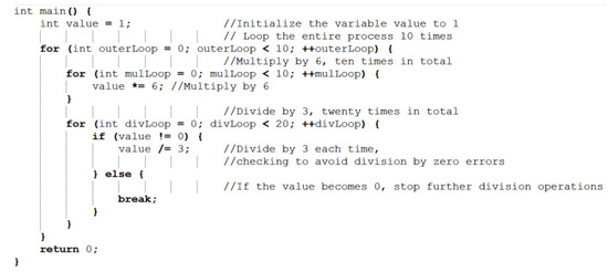
Figure 16. C language test program code for division test case.

The part of the main function from the disassembled file generated by compiling with the RISC-V toolchain (Eclipse) is shown in Figure 17.

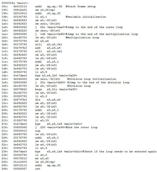
Figure 17. Disassembled instruction code corresponding to the division test case.

Download the generated instruction file into the processor and use ModelSim SE-64 10.5 to perform simulation testing on the processor. A screenshot of data collected during a simulation is shown in Figure 18.

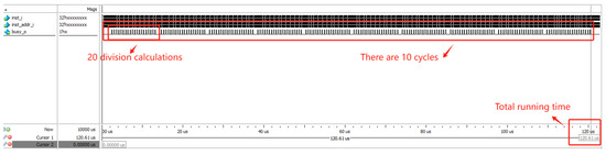
Figure 18. Simulation screenshot of the processor running the division test case.

Run the test 100 times and collect the execution time for each run. The statistics of the execution times are shown in Table 13 (since the fluctuations in execution time are primarily due to the success or failure of branch prediction, and because this test case involves a small total number of conditional branch jump instructions, the resulting data variation is minimal).

Table 13. Test data for Rev-riscv and Rev-riscv-II when running the division test program.

Test Item	Rev-Riscv	Rev-Riscv-II
Number of Tests	100	100
Mean Runtime	269.85 µs	123.24 µs
Variance of Runtime	2.74826 × 10−11	2.47469 × 10−11
Hrtp Value (Convert the unit from microseconds to seconds)	−8.2173	−8.9997

4.3.3. Summary of Real-Time Testing

The resource usage comparison between the two processors is shown in Table 14.

Table 14. Resource consumption data for Rev-riscv and Rev-riscv-II.

Resource Name	Rev-Riscv	Rev-Riscv-II
LUT	11,203	15,161
LUTRAM	4200	4241
FF	6211	6428
IO	18	18

Based on the comprehensive analysis of the experimental results, when executing the Task A test program (CoreMark test program), the hardware real-time parameter H_rtp before optimization was 4.4001 (mean: 77.01907 s, variance: 3.47505). After optimization, under the same program execution conditions, the H_rtp value decreased to 4.3651 (mean: 74.69959 s, variance: 2.95681). Analyzing from the perspective of mean and variance, there is an improvement in the processor’s real-time performance.

The improvement is not significant for the following reasons:

• The final H_rtp value undergoes a logarithmic operation. During the design of H_rtp, considering that the execution time for embedded processors running test tasks is generally less than 1 s, a logarithmic operation was adopted to highlight small optimizations.
• In the CoreMark benchmark test program, the improvement in time data is not significant (approximately only a 3 s reduction, with a total duration exceeding 70 s), leading to less noticeable optimization in program execution speed. In the subsequent division test case, however, there is a more substantial change in the H_rtp value.

When executing the Task B test program (division test program), the hardware real-time parameter H_rtp was −8.2173 before optimization. After optimization, under the same program execution conditions, the H_rtp value decreased to −8.9997, showing an improvement of 0.7824, indicating an enhancement in the processor’s real-time performance.

In conclusion, the analysis demonstrates that the optimized Rev-riscv-II processor shows improved hardware real-time performance under the assumed real-time system requirements for an automotive autonomous driving system. This aligns with the expected theoretical results, suggesting that H_rtp is a reliable metric for evaluating the real-time performance of hardware processors.

In addition, we used the CoreMark benchmark suite to test the performance of the two processors. We also compared their performance with that of similar-level processors, as shown in Table 15. The performance of the Rev-riscv-II processor is superior to that of the Hummingbird E203 [22] and lies between that of Cortex M0+ [24] and Cortex M3 [24]. Compared to the Rev-riscv processor before optimization, the performance improvement is approximately 5.1%.

Table 15. The CoreMark test results for similar-level processors.

Features	CoreMark/MHz
Hummingbird E203 [22]	2.14
Cortex M0 [24]	2.33
Cortex M0+ [24]	2.46
Cortex M3 [24]	3.53
Rev-riscv	2.57
Rev-riscv-II	2.70

5. Conclusions and Future Work

5.1. Summary and Comparison of WCET and H_rtp

The current mainstream methods for evaluating real-time systems primarily focus on Worst-Case Execution Time (WCET) analysis. The WCET and H_rtp analysis methods differ in their analytical objectives and scope. WCET analysis focuses solely on “speed” (the smaller the WCET, the faster the execution), whereas H_rtp analyzes both “speed” and “stability”. Therefore, it is not feasible to conduct a relatively fair quantitative comparison between the two. From a qualitative perspective, each method has its unique advantages.

Advantages of H_rtp Analysis:

• H_rtp analysis applies specifically to hardware components such as processors and interface control hardware, enabling a focused real-time evaluation of hardware alone (only needing to meet predefined requirements). This facilitates the independent development and testing of hardware during the real-time system development process. In contrast, WCET analysis requires comprehensive information about the entire real-time system, including both software and hardware aspects.
• H_rtp extends and refines WCET assessment specifically for hardware evaluation. The calculation of H_rtp utilizes the results of WCET analysis (i.e., T_wcet), making it not only an indicator of whether hardware meets system real-time requirements but also reflecting the degree of “real-time” performance quality when these requirements are met.

Advantages of WCET Analysis:

• WCET analysis has a longer history and covers nearly all types of real-time systems.
• Based on WCET analysis methods, several mature commercial software tools have been developed, offering reliable and convenient solutions.
• Research into WCET analysis algorithms and related topics has developed rapidly.

Undoubtedly, the H_rtp parameter analysis method proposed in this paper falls short of WCET in both application scope and development history.

However, with the large-scale application and development of real-time systems in areas such as the Internet of Things (IoT) and unmanned aerial vehicle (UAV) systems, there is a growing need to evaluate the “goodness” and “badness” of processors and real-time systems. Therefore, we believe that the application of the H_rtp parameter analysis method will gradually increase in future developments.

5.2. Experimental Conclusions and Summary

We conducted research and innovation on the concept of “real-time performance” for processor hardware. We propose a “Hardware Real-Time Performance Parameter (H_rtp)”. This parameter not only reflects whether the hardware can meet the real-time requirements of the system but also evaluates the quality of real-time performance when these requirements are met. We validated the reasonableness of this parameter using data from the processor before and after real-time optimization.

We optimized the branch prediction module of the processor and innovatively proposed a “Simplified Local Branch History Predictor (SLBHP)”. The comparative experiment shows that, with an additional consumption of approximately 2700 logic units, the predictor’s accuracy for conditional branch prediction is 12% higher than that of a static branch predictor. The division calculation of the processor has been optimized. The experiments show that, with an additional consumption of approximately 1200 logic units, the computation speed of the optimized division module can be improved by more than 75%. Through these two optimizations, the processor’s execution time and execution time variability can be effectively reduced, thereby enhancing the “hardware real-time performance” of the processor.

The final experiments showed that when running the CoreMark benchmark program, the processor’s average execution time decreased by 3%, and the execution time variability (variance) decreased by 21%, indicating an improvement in the “quality of hardware real-time performance”. The “Hardware Real-Time Performance Parameter (H_rtp)” changed from 4.4001 to 4.3651, consistent with the trend of improved hardware real-time performance. When executing the self-test program instructions for division, the “Hardware Real-Time Parameter (H_rtp)” decreased from −8.2173 to −8.9997.

The results of running both test programs are consistent with the trend of improved hardware real-time performance. The parameter has a certain reference significance for evaluating “hardware real-time performance”.

Additionally, we compared the performance of the Rev-riscv-II with that of currently mainstream embedded processors, demonstrating that the Rev-riscv-II processor has significant usability.

5.3. Future Work

In the future, we plan to collect operational data from various RISC-V processors and analyze these data using the “Hardware Real-Time Parameter (H_rtp)”. Based on this analysis, we aim to iteratively optimize the formula for H_rtp to continuously improve its accuracy and applicability. The author’s team is preparing for related work, with ongoing projects focusing on processors such as the C910 (RISC-V architecture) and the Xiangshan processor. As more students engage in relevant research, our team will gather real-time test data for different embedded systems. We plan to open-source these data in the future to provide a valuable resource for researchers.

In addition to the application of H_rtp in embedded processors, our team is also conducting research on optimizing airborne real-time networks. Moving forward, we plan to apply the H_rtp analysis method to real-time airborne networks and other relevant fields. We will continuously iterate and optimize the parameter based on the specific requirements of different real-time systems, ensuring its applicability and effectiveness across a broader range of applications.

References

- Kang, J.; Waddington, D.G. Load Balancing Aware Real-Time Task Partitioning in Multicore Systems. In Proceedings of the 2012 IEEE International Conference on Embedded and Real-Time Computing Systems and Applications, Seoul, Republic of Korea, 19–22 August 2012; IEEE: Piscataway, NJ, USA, 2012; pp. 404–407. [Google Scholar]
- Stankovic, J. Misconceptions about Real-Time Computing: A Serious Problem for Next-Generation Systems. Computer 1988, 21, 10–19. [Google Scholar] [CrossRef]
- Lee, E.A. What is Real Time Computing? A Personal View. IEEE Design Test 2018, 35, 64–72. [Google Scholar] [CrossRef]
- Gong, X.; Jiang, B.; Chen, X.; Gao, Y.; Li, X. Survey of Real-Time Computer System Architecture. J. Comput. Res. Dev. 2023, 60, 1021–1036. [Google Scholar] [CrossRef]
- Kohútka, L.; Vojtko, M.; Krajcovic, T. Hardware Accelerated Scheduling in Real-Time Systems. In Proceedings of the 2015 4th Eastern European Regional Conference on the Engineering of Computer Based Systems, Brno, Czech Republic, 27–28 August 2015; IEEE: Piscataway, NJ, USA, 2015; pp. 142–143. [Google Scholar]
- Thiele, L.; Wilhelm, R. Design for Timing Predictability. Real Time Syst. 2004, 28, 157–177. [Google Scholar] [CrossRef]
- Kirner, R.; Puschner, P. Time-Predictable Computing. In Proceedings of the Software Technologies for Embedded and Ubiquitous Systems; Springer: Berlin/Heidelberg, Germany, 2010; pp. 23–34. [Google Scholar]
- Davis, R.I.; Burns, A. A Survey of Hard Real-Time Scheduling for Multiprocessor Systems. ACM Comput. Surv. 2011, 43, 1–44. [Google Scholar] [CrossRef]
- Buttazzo, G.C.; Bertogna, M.; Yao, G. Limited preemptive scheduling for real-time systems. a survey. IEEE Trans. Ind. Inform. 2012, 9, 3–15. [Google Scholar] [CrossRef]
- Engblom, J.; Ermedahl, A.; Sjödin, M.; Gustafsson, J.; Hansson, H. Worst-Case Execution-Time Analysis for Embedded Real-Time Systems. Int. J. Softw. Tools Technol. Transf. 2003, 4, 437–455. [Google Scholar] [CrossRef]
- Pellizzoni, R.; Caccamo, M. Impact of Peripheral-Processor Interference on WCET Analysis of Real-Time Embedded Systems. IEEE Trans. Comput. 2009, 59, 400–415. [Google Scholar] [CrossRef]
- Chen, G.; Guan, N.; Lü, M.S.; Wang, Y. State-of-the-Art Survey of Real-Time Multicore Systems. J. Softw. 2018, 29, 2152–2176. [Google Scholar]
- Dreyer, B.; Hochberger, C.; Wegener, S. Call String Sensitivity for Hardware-Based Hybrid WCET Analysis. IEEE Embed. Syst. Lett. 2021, 14, 91–94. [Google Scholar] [CrossRef]
- Zhang, M.; Gu, Z.; Li, H.; Zheng, N. WCET-Aware Control Flow Checking with Super-Nodes for Resource-Constrained Embedded Systems. IEEE Access 2018, 6, 42394–42406. [Google Scholar] [CrossRef]
- Shah, H.; Huang, K.; Knoll, A. The Priority Division Arbiter for Low WCET and High Resource Utilization in Multi-Core Architectures. In Proceedings of the 22nd International Conference on Real-Time Networks and Systems, Versaille, France, 8–10 October 2014; pp. 247–256. [Google Scholar]
- Li, M.; Xiao, K.; Zhou, Y.; Huang, D. WCET Analysis Based on Micro-Architecture Modeling for Embedded System Security. Appl. Sci. 2024, 14, 7277. [Google Scholar] [CrossRef]
- Herbegue, H.; Cassé, H.; Filali, M.; Rochange, C. Hardware Architecture Specification and Constraint-Based WCET Computation. In Proceedings of the 2013 8th IEEE International Symposium on Industrial Embedded Systems (SIES), Porto, Portugal, 19–21 June 2013; pp. 259–268. [Google Scholar]
- Mancuso, R.; Pellizzoni, R.; Tokcan, N.; Caccamo, M. WCET Derivation Under Single Core Equivalence with Explicit Memory Budget Assignment. In Proceedings of the 29th Euromicro Conference on Real-Time Systems (ECRTS 2017), Dubrovnik, Croatia, 27–30 June 2017. [Google Scholar]
- Seifert, G. Static Analysis Methodologies for WCET Calculating with Asynchronous IO. In Proceedings of the Software Engineering 2022 Workshops, Berlin, Germany, 21–25 February; pp. 115–127.
- Abella, J.; Hernández, C.; Quiñones, E.; Cazorla, F.J.; Conmy, P.R.; Azkarate-Askasua, M.; Perez, J.; Mezzetti, E.; Vardanega, T. WCET Analysis Methods: Pitfalls and Challenges on Their Trustworthiness. In Proceedings of the 10th IEEE International Symposium on Industrial Embedded Systems (SIES), Siegen, Germany, 8–10 June 2015; IEEE: Piscataway, NJ, USA, 2015; pp. 1–10. [Google Scholar]
- Wei, Q.; Cui, E.; Gao, Y.; Li, T. A Review of Edge Intelligence Applications Based on RISC-V. In Proceedings of the 2023 2nd International Conference on Computing, Communication, Perception and Quantum Technology (CCPQT), Xiamen, China, 4–7 August 2023; pp. 115–119. [Google Scholar] [CrossRef]
- Wei, Y.; Yang, Z.; Tie, J.; Shi, W.; Zhou, L.; Wang, Y.; Wang, L.; Xu, W. A Multistage Dynamic Branch Predictor Based on Hummingbird E203. Comput. Eng. Sci. 2024, 46, 785. [Google Scholar]
- Lu, Z.; Lach, J.; Stan, M.R.; Skadron, K. Alloyed Branch History: Combining Global and Local Branch History for Robust Performance. Int. J. Parallel Program. 2003, 31, 137–177. [Google Scholar] [CrossRef]
- Martin, T. The Designer’s Guide to the Cortex-M Processor Family; Newnes: Boston, MA, USA, 2022. [Google Scholar]
Disclaimer/Publisher’s Note: The statements, opinions and data contained in all publications are solely those of the individual author(s) and contributor(s) and not of MDPI and/or the editor(s). MDPI and/or the editor(s) disclaim responsibility for any injury to people or property resulting from any ideas, methods, instructions or products referred to in the content. |
© 2025 by the authors. Licensee MDPI, Basel, Switzerland. This article is an open access article distributed under the terms and conditions of the Creative Commons Attribution (CC BY) license (https://creativecommons.org/licenses/by/4.0/).