MRI Boundary-Aware Segmentation of Multiple Sclerosis Lesions Using a Novel Mahalanobis Distance Map

Abstract

The accurate segmentation of multiple sclerosis (MS) lesions in magnetic resonance imaging (MRI) is essential for diagnosis, disease monitoring, and therapeutic assessment. Despite the significant advances in deep learning-based segmentation, the current boundary-aware approaches are limited by their reliance on spatial distance transforms, which fail to fully exploit the rich texture and intensity information inherent in MRI data. This limitation is particularly problematic in regions where MS lesions and normal-appearing white matter exhibit overlapping intensity distributions, resulting in ambiguous boundaries and reduced segmentation accuracy. To address these challenges, we propose a novel Mahalanobis distance map (MDM) and a corresponding Mahalanobis distance loss, which generalize traditional distance transforms by incorporating spatial coordinates, the FLAIR intensity, and radiomic texture features into a unified feature space. Our method leverages the covariance structure of these features to better distinguish ambiguous regions near lesion boundaries, mimicking the texture-aware reasoning of expert radiologists. Experimental evaluation on the ISBI-MS and MSSEG datasets demonstrates that our approach achieves superior performance in both boundary quality metrics (HD95, ASSD) and overall segmentation accuracy (Dice score, precision) compared to state-of-the-art methods. These results highlight the potential of texture-integrated distance metrics to overcome MS lesion segmentation difficulties, providing more reliable and reproducible assessments for MS management and research.

1. Introduction

Multiple sclerosis (MS) lesion segmentation is a critical task in medical imaging. MS is a chronic autoimmune disease of the central nervous system, marked by white matter lesions that disrupt myelin and axons, causing progressive neurological deficits [1]. Magnetic resonance imaging (MRI) is the standard tool for the detection and monitoring of MS lesions, relying on T1-weighted (T1-w), T2-weighted (T2-w), proton density-weighted (PD-w), and fluid-attenuated inversion recovery (FLAIR) sequences. On MRI, MS lesions typically appear as hyperintense regions in T2-w, PD-w, and FLAIR scans and as hypointense regions in T1-w images.

Accurate lesion segmentation on MRI is essential for the quantitative assessment of disease progression and therapeutic monitoring [2]. Clinicians require reliable lesion quantification for diagnosis, treatment planning, prognosis, and drug development [3,4]. However, manual delineation remains labor-intensive, subject to inter-rater variability, and difficult even for expert neuroradiologists due to the subtle and heterogeneous lesion appearance across scans [2,5]. Ambiguous lesion boundaries, partial volume effects [6], and their overlap with normal tissue complicate human interpretation and simultaneously expose the limitations of automated segmentation algorithms, whose performance is degraded by class imbalances [7], intensity variability [7], and overlapping intensity distributions [8,9,10,11,12]. Consequently, both expert observers and computational models often yield inconsistent delineations, with increased false positives and negatives, especially at lesion margins.

To mitigate these challenges, recent research has increasingly focused on convolutional neural networks (CNNs), with U-Net architectures emerging as the dominant paradigm given their demonstrated efficacy in biomedical image segmentation [13,14,15]. Contemporary approaches extend this framework by integrating probabilistic modeling [16], exploiting lesion-specific contrasts such as FLAIR hyperintensities [17], and incorporating spatial–spectral lesion features [18]. In parallel, boundary-aware loss functions have been proposed to address systematic errors arising from class imbalances and poorly defined lesion borders. In contrast to conventional region-based metrics such as the Dice loss [19], these functions leverage distance transforms to weight prediction errors relative to their proximities to lesion boundaries, thus enhancing the segmentation accuracy through the explicit integration of geometric cues [20,21,22,23].

Despite the significant progress in boundary-aware segmentation techniques, the current methods remain constrained by two fundamental limitations. First, the small size of typical MS lesions results in a limited number of boundary voxels, causing instability during training and hindering effective generalization. Second, these approaches predominantly rely on spatial distance metrics (e.g., Euclidean-based transforms) that frequently fail to leverage the rich texture and intensity information from MRI data. This dual limitation impedes the accurate delineation of ambiguous regions near lesion boundaries, particularly where intensity distributions overlap between lesions and normal-appearing white matter [20,21,22,23].

In this work, we introduce a Mahalanobis distance map (MDM) framework for MS lesion segmentation, which extends traditional distance transform methods by combining spatial coordinates, FLAIR intensities, and radiomic texture features into a voxel-level feature vector [24]. The Mahalanobis distance, computed using a graphical lasso-estimated precision matrix [25], serves as a robust dissimilarity measure, especially advantageous for small boundary samples and correlated feature spaces. By adaptively weighting ambiguous boundaries through radiomic features and integrating volumetric and boundary optimization via a decaying coefficient, our method achieves improved lesion delineation even in regions where intensity distributions overlap.

Our main contributions, with respect to the main MS segmentation challenges (class imbalance [7], partial volume effects [6], intensity heterogeneity [7], and overlapping intensities [8,9,10,11,12]), are as follows.

• Generalization of boundary-aware loss: We extend the boundary loss framework [22] by incorporating local texture information, which improves the boundary localization and segmentation performance, especially in cases suffering from overlapping intensity distributions and partial volume effects.
• Texture-integrated distance metric: By replacing traditional Euclidean-based transforms with a Mahalanobis distance map, our method leverages spatial, intensity, and texture attributes. This enhancement addresses the problem of ambiguous boundaries caused by partial volume effects and overlapping intensities, as the covariance-aware metric distinguishes subtle texture differences at lesion edges more effectively.
• Dynamic feature weighting and hybrid optimization: The adaptive weighting of ambiguous boundary regions using radiomic features allows the model to focus more precisely on difficult-to-segment areas. Additionally, our use of a decaying coefficient shifts learning progressively from region-focused to boundary-focused optimization, helping to stabilize training where class imbalance and sparse boundary voxels would otherwise disrupt convergence.

The paper is organized as follows. Section 2 reviews the relevant background and the main loss functions used in medical image segmentation tasks. Section 3 introduces our proposed approach, consisting of the Mahalanobis distance map and Mahalanobis distance loss. Section 4 presents and discusses experimental results obtained on the 2015 Longitudinal MS Lesion Segmentation Challenge (ISBI-MS) and Multiple Sclerosis Segmentation Challenge (MSSEG) datasets. Finally, Section 6 concludes the work and outlines future research directions.

For reproducibility, all code and implementation details are available at https://github.com/GustavoUlloaPoblete/MSLesionSegmentation (accessed on 28 September 2025).

2. Related Work

Let us consider the image segmentation problem, where the goal is to partition the image domain $\Omega \subset {\mathbb{N}}^2$ into meaningful regions, typically distinguishing between the foreground (objects of interest, such as lesions or anatomical structures) and background. Given an image as a function $I_{H\times W}:\Omega \to {\mathbb{R}}_{H\times W}^D$ [26], with each spatial coordinate $p:=(h,w)\in \Omega$ mapped to a feature vector $I\left(p\right)\in {\mathbb{R}}^D$, where D corresponds to the number of channels of the $H\times W$ image, the task is to assign a label to every voxel, where a voxel is defined as a pair $(p,I(p\left)\right)$, so that regions with similar characteristics are grouped together.

For binary segmentation, the task involves learning a mapping $G_{H\times W}:I_{H\times W}\to {\{0,1\}}_{H\times W}$ (typically provided by expert annotations) that assigns a binary label to each voxel in the image domain $\Omega$. Here, $G\left(p\right)=1$ indicates foreground membership (e.g., a lesion or anatomical structure), while $G\left(p\right)=0$ corresponds to the background. A segmentation model, such as a neural network, produces a probabilistic output ${s_{\theta }}_{H\times W}:I_{H\times W}\to {[0,1]}_{H\times W}$, estimating the likelihood of each voxel belonging to the foreground. The ground-truth boundaries ($GB$), representing the edges of the foreground region, are derived from G. Similarly, predicted boundaries (PB) are obtained from the automatic segmentation P, which is derived after thresholding the network’s output at $P=s_{\theta }>0.5$, a common practice to generate discrete segmentations from probabilistic predictions [20,27].

In the context of multiple sclerosis lesion segmentation, a central challenge is to accurately delineate lesion boundaries within brain MRI scans, particularly when lesions overlap with or resemble surrounding tissues, leading to ambiguous region distinctions. Precise boundary estimation is essential for reliable clinical assessment and research, as it enables the meaningful extraction and quantitative analysis of the disease burden and progression. To address these complexities, recent approaches have incorporated distance maps into loss functions during model training [20,21,22,23]. These maps are generated by transforming the ground-truth mask G into a representation where each voxel encodes the Euclidean distance to the nearest boundary voxel in the set $GB$. Formally, the distance transform map (DTM) is defined as [20,21]

$$DTM(x,G)=\left\{\begin{array}{ccc}\hfill {\displaystyle \underset{y\in GB}{inf}{\{\parallel x-y\parallel }_2\}}& \mathrm{if}& x\in G_{in}\cup G_{out},\hfill \\ \hfill 0& \mathrm{if}& x\in GB,\hfill \end{array}\right.$$

(1)

where ${\parallel x-y\parallel }_2$ denotes the Euclidean distance between voxels x and y, and $G_{in}$, $G_{out}$ represent voxels inside and outside the lesion, respectively.

To further refine boundary-aware training, the signed distance function (SDF) extends the concept of distance transforms by encoding directional information relative to the lesion boundary. The SDF is defined as [22]

$$SDF(x,G)=\left\{\begin{array}{ccc}\hfill {\displaystyle -\underset{y\in GB}{inf}{\{\parallel x-y\parallel }_2\}}& \mathrm{if}& x\in G_{in},\hfill \\ \hfill 0& \mathrm{if}& x\in GB,\hfill \\ \hfill {\displaystyle \underset{y\in GB}{inf}{\{\parallel x-y\parallel }_2\}}& \mathrm{if}& x\in G_{out}.\hfill \end{array}\right.$$

(2)

Thus, unlike the DTM, the SDF assigns negative values to the distances of voxels inside the object $G_{in}$. For simplicity, the DTM and SDF transforms of G are denoted as $G_{DTM}$ and $G_{SDF}$, respectively. Integrating such distance-based representations into loss functions helps segmentation models to better capture the subtle and complex boundaries characteristic of MS lesions, ultimately improving the accuracy and robustness of automated lesion quantification [20,22].

Segmentation models leveraging boundary-aware distance transforms such as the DTM and SDF face inherent optimization challenges during early training stages. Due to the high variability in initial predictions, where neural networks produce unstable object boundaries and noisy foreground probabilities, directly applying boundary-based loss functions (e.g., those using $G_{DTM}$ or $G_{SDF}$) often leads to gradient explosion or erratic convergence patterns. This instability arises because boundary terms disproportionately penalize large errors in regions where the network’s probabilistic predictions ($s_{\theta }$) are still poorly calibrated, creating conflicting gradient signals.

To mitigate this, recent methodologies adopt a hybrid loss framework that progressively transitions the optimization focus from region-aware to boundary-aware objectives [20,22,23]. The approach combines a region-aware loss component, denoted by $L_{\mathrm{region}\text{-}\mathrm{aware}}$ (e.g., generalized Dice loss $L_{\mathrm{GDice}}$, which leverages global statistics for volumetric coherence [19]), with a boundary-aware loss term, denoted by $L_{\mathrm{boundary}\text{-}\mathrm{aware}}$ (e.g., edge alignment via Hausdorff distance loss [20] or boundary loss [22]), through a decaying coefficient $ϵ$

$$L=ϵ·L_{\mathrm{region}\text{-}\mathrm{aware}}+(1-ϵ)·L_{\mathrm{boundary}\text{-}\mathrm{aware}},$$

(3)

where $ϵ$ linearly decreases from $1.0$ to $0.01$ over the training epochs, enabling initial stabilization through region-based metrics before sharpening the boundary precision. In the early phases, the region-aware term dominates, ensuring robust foreground–background separation by optimizing overlap metrics. As $ϵ$ diminishes, the boundary-aware term gradually takes precedence, refining structural edges by aligning the predicted boundaries ($PB$) with ground-truth anatomical contours ($GB$). This dual-phase strategy harmonizes complementary goals: establishing volumetric stability first, followed by enhancing the fine-grained geometric accuracy and ultimately balancing segmentation robustness and detail preservation.

Building on this foundation, contemporary segmentation losses can be categorized into three main paradigms: distribution-based losses, region-based losses, and boundary-aware losses. Each category addresses distinct aspects of the segmentation problem, as explored in the following sections [28].

2.1. Distribution-Based Loss

Binary Cross-Entropy Loss

The binary cross-entropy loss function is defined as [29]

$$L_{BCE}(G,s_{\theta })=-\sum _{p\in \Omega }\left(G\left(p\right)·log\left(s_{\theta }\left(p\right)\right)+(1-G\left(p\right))·log(1-s_{\theta }\left(p\right))\right),$$

(4)

which originates from information theory’s entropy formulation, comparing the true distribution $G\left(p\right)$ with the estimated distribution $s_{\theta }\left(p\right)$ using the cross-entropy term. While binary cross-entropy remains a standard choice for binary segmentation tasks, its application to MS lesion segmentation faces challenges due to extreme class imbalance (lesions often occupy less than 1% of the brain volume), causing binary cross-entropy to prioritize background voxels, leading to the under-segmentation of small lesions.

2.2. Region-Based Loss

2.2.1. Dice Loss

The Dice loss function [30] is based on the Dice score (or F1-score), which measures the overlap between the predicted segmentation s and the ground-truth mask G. It is widely used in medical image segmentation tasks, especially for problems with class imbalance, such as MS lesion segmentation. The Dice loss is defined as

$$L_{Dice}(G,s_{\theta })=1-{\displaystyle \frac{2{\sum }_{p\in \Omega }G\left(p\right)s_{\theta }\left(p\right)}{{\sum }_{p\in \Omega }G{\left(p\right)}^2+{\sum }_{p\in \Omega }{s}_{\theta }{\left(p\right)}^2}}.$$

(5)

While the Dice loss delivers strong overlap metrics for MS lesion segmentation, its performance is unstable for small or sparse lesions and highly imbalanced datasets, often resulting in missed detections or segmentation errors.

2.2.2. Generalized Dice Loss

To address these limitations, the generalized Dice loss (GDice) [19] introduces class-specific weights that are inversely proportional to their prevalence, thereby enhancing the robustness to extreme class imbalances and improving the detection of subtle lesions. The loss is defined as

$$L_{GDice}(G,s_{\theta })=1-2{\displaystyle \frac{{\displaystyle \sum _{l=1}^2{w}_l\sum _{p\in \Omega }{G}_{\left(l\right)}\left(p\right)s_{\theta ,\left(l\right)}\left(p\right)}}{{\displaystyle \sum _{l=1}^2{w}_l\sum _{p\in \Omega }\left(G_{\left(l\right)}\left(p\right)+s_{\theta ,\left(l\right)}\left(p\right)\right)}}}$$

(6)

where $w_l=1/{\left({\sum }_{p\in \Omega }{G}_{\left(l\right)}\left(p\right)\right)}^2$, and $\left(l\right)$ denotes the class index.

2.3. Boundary-Based Loss

2.3.1. Hausdorff Distance Loss

The Hausdorff distance loss function is utilized to minimize the maximum boundary discrepancy between two objects, with a particular emphasis on reducing the largest separation between the predicted and ground-truth boundaries in MS segmentation tasks. The bidirectional Hausdorff distance is calculated between two binary sets, denoted as G and P.

$$\mathrm{HD}(G,P)=max\left(\mathrm{hd}(G,P),\mathrm{hd}(P,G)\right),$$

(7)

where

$$\mathrm{hd}(X,Y)=\underset{x\in G}{max}\underset{y\in P}{min}{\parallel x-y\parallel }_2$$

(8)

is the unidirectional Hausdorff distance.

In [20], the authors define a Hausdorff distance-based loss function that incorporates the distance transform (DTM) of Equation (1), maps of both the ground-truth segmentation mask, denoted as $G_{DTM}$, and the automatic segmentation, denoted as $P_{DTM}$. The loss function is formulated as follows:

$$L_{HD}(G,s_{\theta })=ϵ·L_{GDice}+(1-ϵ)·{\displaystyle \frac{1}{|\Omega |}}\sum _{p\in \Omega }{(G\left(p\right)-s_{\theta }\left(p\right))}^2·(G_{DTM}^2\left(p\right)+P_{DTM}^2\left(p\right)),$$

(9)

where $L_{GDice}$ represents the generalized Dice loss term, $|\Omega |$ denotes the total number of voxels, and $ϵ$ is a weighting parameter that balances the contributions of the terms based on the region and the boundaries (see Equation (3)). This formulation, which combines global overlap optimization through the Dice loss with a boundary-focused penalty weighted by distance transform maps, is especially appropriate given the small size, irregular shape, and scattered distribution of MS lesions, as these characteristics make precise boundary delineation difficult.

2.3.2. Boundary Loss

The boundary loss is another alternative to traditional region-based loss functions, specifically designed to address the challenges of highly unbalanced segmentation tasks [22]. The boundary loss is defined as

$$L_B(G,s_{\theta })=ϵL_{GDice}+(1-ϵ)·{\displaystyle \frac{1}{|\Omega |}}\sum _{p\in \Omega }{G}_{SDF}\left(p\right)s_{\theta }\left(p\right),$$

(10)

where $G_{SDF}$ denotes the signed distance function of the ground-truth mask G (see Equation (2)). In this formulation, $L_{GDice}$ is the generalized Dice loss, and $s_{\theta }\left(p\right)$ is the predicted probability at voxel p.

Unlike conventional losses that sum over entire regions, which can be problematic when there is a large class imbalance, the boundary loss focuses on the interface between regions, i.e., the object boundaries. This approach allows the model to directly optimize for accurate boundary localization, mitigating the dominance of the majority class and improving the segmentation performance, especially for small or irregular structures.

2.3.3. Boundary-Sensitive Loss

The boundary-sensitive loss was proposed to address intra-class imbalances in the segmentation of objects of interest, such as MS lesions, where boundaries are often diffuse and difficult to delineate [31]. This loss penalizes false positives and false negatives at the internal and external boundaries of both the ground truth (${\mathrm{FBG}}_{in}$, ${\mathrm{FBG}}_{out}$) and the prediction (${\mathrm{FBP}}_{in}$, ${\mathrm{FBP}}_{out}$), as well as within the interiors of these regions ($\mathrm{FIG}$ and $\mathrm{FIP}$). The loss is given by

$$\begin{array}{cc}\hfill {\mathrm{WF}}^P& =\alpha ·({\mathrm{FBP}}_{in}+{\mathrm{FBG}}_{out})+(1-\alpha )·\mathrm{FIP}\hfill \end{array}$$

(11)

$$\begin{array}{cc}\hfill {\mathrm{WF}}^G& =\alpha ·({\mathrm{FBP}}_{out}+{\mathrm{FBG}}_{in})+(1-\alpha )·\mathrm{FIG}\hfill \end{array}$$

(12)

where $\alpha >0.5$ increases the penalty for errors at the internal and external boundaries compared to errors in the interior. This weighting is implemented in a Dice-like loss function by replacing the standard false positive and false negative terms:

$$L_{BS}=1-{\displaystyle \frac{2TIG}{2TIG+{\mathrm{WF}}^P+{\mathrm{WF}}^G}},$$

(13)

where TIG corresponds to the true positives. The boundary-sensitive loss is designed to improve the segmentation of challenging or poorly defined boundaries, such as those found in medical images, by allowing emphasis to be placed on boundary errors through a tunable parameter and an optional location constraint for added robustness; however, its effectiveness can be limited in MS imaging due to the diffuse nature of lesion edges, potential training instability, and the risk of over-penalizing minor boundary inaccuracies.

2.3.4. Active Boundary Loss

In [23], the authors propose the active boundary loss function, which aims to improve the alignment between $PB$ and $GB$. This loss function is formulated as a problem of predicting the direction vector of voxels on $PB$ towards $GB$, thereby guiding the movement of $PB$ during training epochs. This is achieved by minimizing the Kullback–Leibler divergence between the class probability distribution of a voxel $u=(i,j)$ on $PB$ and its neighboring voxel $v=(i+\mathrm{\Delta }i,j+\mathrm{\Delta }j)$, which is the closest candidate to $GB$ according to the Euclidean distance transform map DTM (see Equation (1)).

As with the Hausdorff distance loss and boundary loss, the implementation of this loss function is performed as a convex linear combination with $L_{GDice}$:

$$L_{AB}(G,s_{\theta })=ϵ·L_{GDice}+(1-ϵ)·{\displaystyle \frac{1}{\left|PB\right|}}\sum _{q\in PB}\mathsf{\Lambda }\left(G_{DTM}\left(q\right)\right)·CE(D^p\left(q\right),D^g\left(q\right)).$$

(14)

where $\mathsf{\Lambda }$ is a function of the $G_{DTM}$ distance map that weights the cross-entropy (CE), $D^g\left(q\right)$ is a one-hot vector indicating the neighboring voxel of q with the smallest distance to $GB$, and $D^p\left(q\right)$ is the probability distribution of the predicted direction for the neighborhood of q.

2.3.5. Conditional Boundary Loss

Similar to the active boundary loss, this loss function aims to improve the alignment between $PB$ and $GB$. It operates by considering, for each boundary voxel, the relationships with neighboring voxels within a $5\times 5$ window. The loss function is defined as [32]

$$L_{CB}(G,s_{\theta })=ϵ·L_{GDice}+(1-ϵ)·(L_{A2C}+\beta L_{A2P\&N}),$$

(15)

where the $L_{A2C}$ term measures the discrepancy between each boundary voxel and its well-classified same-class representative within the local neighborhood, combining a pairwise distance component that penalizes misalignment with a cross-entropy term that encourages correct boundary classification. The $L_{A2P\&N}$ term, weighted by $\beta$, promotes similarity between same-class voxel pairs (A2P) and dissimilarity between adjacent-class pairs (A2N) within the neighborhood. Overall, the parameters $\beta$ and $ϵ$ control the relative contributions of the $L_{CB}$ terms, as well as the trade-off with the generalized Dice loss ($L_{GDice}$). In our experiments, we adopted the recommended values for $\beta$ as suggested in the original formulation [32].

3. Materials and Methods

Our approach aims to better replicate the texture-aware reasoning used by radiologists when segmenting brain MRI lesions by moving beyond traditional distance maps that rely only on Euclidean distances such as the DTM (Equation (1)) and SDF (Equation (2)). To capture the nuanced local texture and intensity context, particularly important in regions with overlapping lesion and background intensities, we introduce the Mahalanobis distance map (MDM, Section 3.1). This method constructs voxel-wise feature vectors combining spatial coordinates, image intensities, and local texture descriptors and measures the distances to lesion or background prototypes using the Mahalanobis distance, which accounts for feature correlations and scale differences. By reflecting both spatial proximity and the statistical similarity of local patterns, the MDM provides a more discriminative and robust signal for training. We further integrate this map into the Mahalanobis distance loss (Section 3.2), which enhances the segmentation performance, especially at ambiguous lesion boundaries.

3.1. Mahalanobis Distance Map

The Mahalanobis distance quantifies the separation between pairs of entities within the same feature space. It remains unaffected by scale and incorporates the covariance among variables [33]. For two vectors (or objects) $x_A$ and $x_B$, the Mahalanobis distance is given by

$$MD(x_A,x_B)=\sqrt{{(x_B-x_A)}^T{C}^{-1}(x_B-x_A)},$$

(16)

where $C^{-1}$ denotes the precision matrix. This distance serves as a measure of the divergence between a new object’s feature vector and a prototype vector that characterizes the dataset’s distribution. It is frequently used to assess whether a new object fits within a data distribution or constitutes an out-of-distribution sample, indicating an outlier.

Algorithm 1 outlines the pseudocode for the procedure to calculate the MDM. In line 2, the process involves creating the feature map $F\in {\mathbb{R}}^{N\times H\times W}$. Here, every voxel p in the image $I\in {\mathbb{R}}^{H\times W}$ is represented as a feature vector $F\left(p\right)\in {\mathbb{R}}^N$ encompassing N features. Line 3 identifies the boundary voxel sets for both the foreground class (GB) and the background class (BB). These sets are crucial for the step in line 4, as they help to define the regions of interest (RoIs) that correspond to the local neighborhoods around each boundary voxel. These neighborhoods are defined by executing a logical AND between a class-specific mask and a spherical mask with radius $r=5$ centered on each boundary voxel of the respective class, as depicted in Figure 1. Considering the 3D nature of brain MRI volumes, to construct this RoI, it is possible to use the slide where the GB and BB sets are located, as well as the adjacent slides where the a parameter defines the number of adjacent slides considered in the spherical mask. If $a=0$, only slide i is considered; however, if $a>0$, slides $[i-a,\dots ,i-1,i,i+1,\dots ,i+a]$ are also considered.

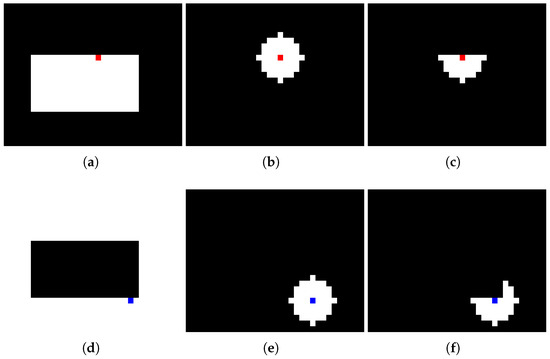
Figure 1. RoI construction process with $a=0$: (a) foreground class mask, (b) circular mask centered on $GB$ edge voxel (red square indicates the selected voxel), (c) resulting foreground RoI, (d) background class mask, (e) circular mask centered on $BB$ edge voxel (blue square indicates the selected voxel), (f) resulting background RoI.

Subsequently, in line 5, for every RoI, both the prototype vector $\tilde{x}$ and the precision matrix $C^{-1}$ are determined. The prototype vector represents the median vector, while the precision matrix is estimated using the graphical lasso algorithm, as described in [25]. This estimator was chosen due to its favorable properties, enabling the estimation of the precision matrix even in datasets with a small sample size and linear dependencies among features and instances. These advantages render the graphical lasso particularly suitable for RoIs with few voxels.

In line 6, the mask H is produced, representing a subset of image voxels comprising the combination of all lesion voxels (denoted as ground truth G) and surrounding background voxels that are within D [mm] of the lesion perimeters:

$$H=G\cup (G_{out}\cap G_{DTM}\le D).$$

(17)

Thus, the MDM aims to detect texture differences not only within lesions but also in the areas surrounding lesion edges. These are the zones where the main difficulties in brain lesion segmentation, such as partial volume effects and overlapping voxel intensity distributions, are encountered and where the majority of false positives and negatives tend to appear. The empirical choice of the value $D=10$ [mm] was determined from the options set $D\in \{5,10,15\}$.

Following this, from lines 7 to 15, the Mahalanobis distance is calculated between each vector $p\in H$ and its respective prototype vector. For example, for each voxel categorized as foreground, the nearest background boundary voxel in $BB$ (determined by the shortest Euclidean distance based on spatial coordinates) is chosen. This selection enables the use of the relevant $\tilde{x}$ and $C^{-1}$ in the Mahalanobis distance computation:

$$\begin{array}{c}\hfill MD(F\left(p\right),\tilde{x})=\sqrt{{(F\left(p\right)-\tilde{x})}^T{C}^{-1}(F\left(p\right)-\tilde{x})}.\end{array}$$

(18)

Algorithm 1 Steps for computing the Mahalanobis distance map (MDM). The algorithm combines texture attributes with a covariance structure to enhance standard distance transforms.

1: Input: $G:\mathrm{Ground}\mathrm{truth}$, $I:\mathrm{FLAIR}\mathrm{modality}$, $a:\mathrm{adjacency}$   2: Compute feature map F   3: Extract boundary voxels for foreground ($GB$) and background boundary ($BB$) sets   4: Define RoIs with adjacency a for each edge voxel in both classes.   5: For each RoI: Compute prototype $\tilde{x}$ and precision matrix $C^{-1}$ using graphical lasso   6: Generate subset H according to Equation (17), i.e., $$H=G\cup (G_{out}\cap G_{DTM}\le D)$$   7: Compute Mahalanobis distances for voxels in H:   8: while For each voxel $p\in H$ in image I do   9:    if $p\in G_{out}\cap H$ then 10:        Find nearest $BG$ edge voxel (Euclidean distance), load $\tilde{x}$ and $C^{-1}$  11:    else if $p\in G_{in}$ then 12:        Find nearest $BB$ edge voxel (Euclidean distance), load $\tilde{x}$ and $C^{-1}$ 13:    end if 14:    Compute: $$\begin{array}{c}\hfill G_{MDM}\left(p\right)=MD(F\left(p\right),\tilde{x})\end{array}$$ (19) 15: end while 16: Output: $G_{MDM}$

3.2. Mahalanobis Distance Loss

According to Algorithm 1, to compute the Mahalanobis distance map, we must first derive the feature map F. This involves obtaining N feature channels from both the ground truth G and the FLAIR modality. From G, we gather two spatial features per voxel, specifically the h and w positions, which are associated with the Euclidean distances used in the traditional distance transform (Equation (1)) and signed distance function (Equation (2)). In addition, we extract intensity values and radiomic texture features from the FLAIR modality, such as the gradient, as well as characteristics from the gray-level co-occurrence matrix (GLCM) [34] and gray-level run-length matrix (GLRLM) [35] detailed in [24].

Texture features are derived from square areas centered around each voxel. For gradient features, $3\times 3$ neighborhoods are used, whereas larger $9\times 9$ neighborhoods are utilized to calculate the 13 GLCM and 11 GLRLM features. To address the curse of dimensionality in precision matrix estimation from limited samples, only the first two principal components of the GLCM and GLRLM features were retained, effectively capturing over $90\%$ of the total variance. Empirical analysis demonstrated that incorporating additional principal components did not improve the segmentation performance and often led to instability in precision matrix estimation. Figure 2 illustrates these features, omitting the spatial coordinates h and w.

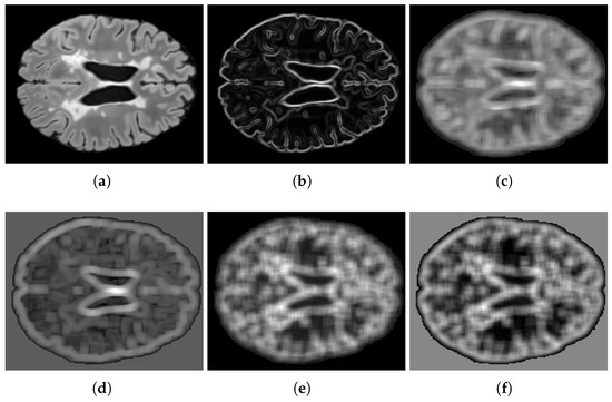
Figure 2. Feature visualization: (a) FLAIR intensity, (b) gradient magnitude, (c,d) GLCM principal components 1–2, (e,f) GLRLM principal components 1–2.

The suggested loss function utilizes the MDM to assign weights to false positives (FP) and false negatives (FN), integrating texture information into the penalty structure. This method is hypothesized to align more closely with radiologists’ implicit reasoning, where local texture insights enhance intensity assessments, especially in areas where intensity distributions overlap due to partial volume effects.

The proposed loss function, termed the Mahalanobis distance loss, is formulated as follows:

$$L_{MDM}(G,s_{\theta })=ϵ·L_{GDice}+(1-ϵ)·{\displaystyle \frac{1}{|\Omega |}}·\sum _{p\in \Omega }{G}_{MDM}^{\lambda }\left(p\right)·\left[(1-G\left(p\right))s_{\theta }\left(p\right)+G\left(p\right)(1-s_{\theta }\left(p\right))\right]$$

(20)

where $G_{MDM}\left(p\right)$ denotes the Mahalanobis distance map’s value at voxel p, $\lambda$ is a non-negative adjustable exponent influencing the relative strength of the penalty, and $ϵ$ linearly decreases from $1.0$ to $0.01$ throughout the training epochs. This approach encourages early stabilization via region-based metrics and subsequently enhances the boundary accuracy progressively.

The parameter $\lambda$ modulates how the penalty scales with respect to the distance map. Specifically, $G_{MDM}{\left(p\right)}^{\lambda }$ acts as a weighting factor that increases or decreases the contribution of a voxel according to its distance from the nearest boundary of the opposing class. When $\lambda >1$, voxels located farther from the class boundary are penalized more heavily, enforcing sharper separation between regions. Conversely, when $0<\lambda <1$, the weighting function is compressed, leading to a milder penalty on distant voxels and a relative emphasis on those closer to the boundary. Figure 3d–f illustrate the Mahalanobis distance maps produced by Algorithm 1 at varying $\lambda$ values. In contrast to the traditional DTM (Figure 3b) and SDF (Figure 3c) maps, our proposed maps allow for a larger range in the distances between voxels near the boundary due to the incorporation of texture features in the distance calculation. From the perspective of classification errors, the term $G_{MDM}\left(p\right)$ penalizes voxels that, given their true class $G\left(p\right)$, lie in the spatial vicinity of the opposite class. This penalty is proportional to the degree of dissimilarity, which tends to be higher for voxels outside lesions compared to voxels inside them. Consequently, the loss formulation biases the optimization toward reducing false positives more strongly than false negatives, as misclassified voxels outside the lesion area (FP) incur higher costs relative to those inside (FN).

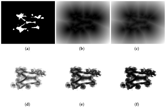
Figure 3. Comparison of distance maps. The figure shows (a) a segmentation mask G and different distance maps: (b) $G_{DTM}$, (c) $G_{SDF}$, and (d–f) $G_{MDM}^{\lambda }$ maps with different values of $\lambda$: (d) $\lambda =0.5$, (e) $\lambda =1.5$, and (f) $\lambda =2.5$.

4. Results

This section provides a succinct evaluation of the loss functions used for the automatic segmentation of brain lesions caused by multiple sclerosis in MRI scans.

4.1. Datasets

The experiments utilized publicly accessible MRI datasets of patients with brain lesions caused by multiple sclerosis.

4.1.1. ISBI-MS

This dataset was employed in the longitudinal multiple sclerosis lesion segmentation challenge during the International Symposium on Biomedical Imaging (ISBI) in 2015 [36]. The training dataset comprises 21 multi-channel MRI volumes from MS patients, each featuring T1-w, T2-w, PD-w, and FLAIR sequences along with their respective segmentation masks.

4.1.2. MSSEG

This dataset was presented at the MICCAI 2016 MS lesion segmentation challenge. It contains MRI volumes, including T1-w, T2-w, and FLAIR modalities, from 15 patients with MS. The ground-truth binary segmentation mask represents a consensus derived from 7 masks produced by various experts [37].

4.2. Preprocessing and Training Setup

Preprocessing encompasses two distinct stages, with each comprising a set of transformations executed on the input image prior to its use as input for the CNN and in Algorithm 1 (refer to Figure 4). The initial stage incorporates standard procedures commonly employed within the research community [36]: bias field correction, skull stripping, dura mater stripping, a second bias field correction, and alignment via rigid-body registration to a 1 mm isotropic MNI template (using the FSL platform libraries [38]). This alignment process utilizes affine transformations, which are characterized by their linear components, such as scaling, rotation, and a translation component, ensuring accurate spatial normalization. From this template, the edges corresponding to background class voxels were trimmed to produce volumes of dimensions $160\times 192\times 160$.

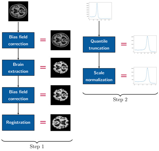
Figure 4. Pipeline of preprocessing steps.

During the second step of preprocessing, image intensities were adjusted to fall within the $[0.01,0.995]$ quantile range, reducing the influence of outliers, and then linearly rescaled to the normalized $[0,1]$ range. For the evaluation of the loss function, we utilized a convolutional autoencoder rooted in the UNet architecture [15], which is the most popular framework for tasks involving medical image segmentation [14]. We opted for transposed convolutions for the upsampling process, rather than interpolation (refer to Figure 5b), which improved the reconstruction of feature maps during the decoding phase. Our CNN utilized a three-channel input corresponding to the T1-w, T2-w, and FLAIR modalities.

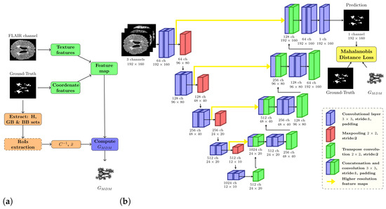
Figure 5. (a) General workflow of Mahalanobis distance map algorithm. (b) Multiple sclerosis lesion segmentation pipeline.

We employed PyTorch [39] as the computational framework to implement the CNN with different loss functions. The training was conducted using four NVIDIA GeForce GTX 1080TI GPUs (each with 11 GB VRAM), which were spread across 4 different servers. This setup required the deployment of a distributed system [40], enabling us to achieve a sufficient number of experimental runs (20 runs). In alignment with the approaches described in [22,23], the models were trained for a maximum of 200 epochs, with early stopping enforced after 30 epochs if the validation set Dice score showed no improvement. This method was essential in preventing overfitting and the degradation of the segmentation results. Although attempts were made to limit the boundary-aware term that predominated in the final training epochs—for example, by setting a minimum value for $\epsilon$, as recommended in the literature [22,23]—early stopping consistently yielded better results across all loss functions.

The optimization process employed the Adam optimizer, set with a learning rate of $0.0001$ and a batch size of 16, determined through empirical methods. For each dataset, only the image slices with lesions were selected for training. These were categorized into three segments: 60% for training, 20% for validation, and 20% for testing. To handle inter-slice correlations within patient volumes, the division was conducted at the patient level rather than at the slice level.

4.3. Evaluation Metrics

In order to measure the effectiveness of various loss functions, we employed a comprehensive range of segmentation metrics, as outlined in [41]. These metrics help to quantify how well the predicted segmentation P aligns with the ground-truth mask G. To evaluate both the boundary precision and the comprehensive segmentation agreement between P and G, we opted for metrics from two primary categories: spatial distance and spatial overlap. For the spatial distance metrics, we implemented the 95th percentile of the Hausdorff distance (HD95) and the average symmetric surface distance (ASSD). For spatial overlap metrics, we incorporated recall (sensitivity), precision (positive predictive value), and the Dice score (equivalent to the F1-score). In addition, we examined the relative volume difference (RVD) and the area under the precision–recall curve (AUC-PR), with the latter being highly effective for datasets with significant imbalance, unlike the more frequently used ROC-AUC. In Table 1, Table 2 and Table 3, the symbols ↓ and ↑ denote whether a decrease or increase in value, respectively, indicates superior performance for each metric.

Table 1. Selection of the hyperparameter $\lambda$ for the ISBI-MS and MSSEG datasets.

	ISBI-MS Dataset
$\mathit{\lambda }$	HD95 (sd)↓	ASSD (sd)↓	Recall (sd)↑	Precision (sd)↑	Dice (sd)↑	rvd (sd)↓	auc-pr (sd)↑
$0.5$	31.947 (9.6748)	3.5236 (1.2628)	0.7127 (0.0398)	0.7281 (0.0730)	0.7132 (0.0346)	0.1541 (0.0930)	0.7205 (0.0317)
$1.0$	31.3346 (11.8639)	3.5310 (1.6014)	0.7101 (0.0308)	0.7446 (0.0709)	0.7199 (0.0291)	0.1647 (0.0479)	0.7274 (0.0285)
$1.5$	27.021 (11.2736)	3.1685 (1.6361)	0.7051 (0.0361)	0.7591 (0.0684)	0.7247 (0.0261)	0.1549 (0.0558)	0.7322 (0.0274)
$2.0$	25.3589 (12.0826)	2.9046 (1.3958)	0.6879 (0.0423)	0.7834 (0.0748)	0.7257 (0.0309)	0.1697 (0.0681)	0.7357 (0.0326)
$2.5$	24.8438 (8.6735)	2.8080 (1.1443)	0.6384 (0.0983)	0.8365 (0.0573)	0.7138 (0.0690)	0.2387 (0.1364)	0.7376 (0.0420)
$3.0$	29.0668 (11.1076)	3.4869 (1.8727)	0.5957 (0.1008)	0.8668 (0.0592)	0.6957 (0.0756)	0.3092 (0.1368)	0.7314 (0.0465)
	MSSEG Dataset
$\mathit{\lambda }$	HD95 (sd)↓	ASSD (sd)↓	Recall (sd)↑	Precision (sd)↑	Dice (sd)↑	rvd (sd)↓	auc-pr (sd)↑
$0.5$	17.4068 (4.0942)	2.5211 (0.4648)	0.6742 (0.0532)	0.6946 (0.0508)	0.6652 (0.0251)	0.3002 (0.0851)	0.6851 (0.0200)
$1.0$	19.393 (4.5113)	2.5342 (0.4190)	0.6866 (0.0380)	0.6967 (0.0556)	0.6743 (0.0197)	0.3071 (0.0762)	0.6923 (0.0159)
$1.5$	17.8207 (5.5012)	2.4039 (0.4239)	0.6868 (0.0412)	0.7039 (0.0508)	0.6794 (0.0184)	0.2802 (0.0656)	0.6960 (0.0153)
$2.0$	17.409 (5.0380)	2.5485 (0.5108)	0.6569 (0.0298)	0.7071 (0.0437)	0.6643 (0.0173)	0.2780 (0.0628)	0.6827 (0.0151)
$2.5$	18.5212 (4.7203)	2.9840 (0.7522)	0.6278 (0.0486)	0.7248 (0.0468)	0.6506 (0.0269)	0.3301 (0.0646)	0.6771 (0.0198)

Table 2. Comparison outcomes on the ISBI-MS dataset (mean and standard deviation from 20 separate runs).

Loss Function	HD95 (sd)↓	ASSD (sd)↓	Recall (sd)↑	Precision (sd)↑	Dice (sd)↑	rvd (sd)↓	auc-pr (sd)↑
$L_{GD}$	31.2239 (11.5185)	4.0412 (2.3260)	0.7210 (0.0382)	0.7082 (0.0873)	0.7055 (0.0502)	0.2005 (0.1808)	0.7147 (0.0406)
$L_{BL}$	30.2914 (09.7484)	3.4456 (1.4219)	0.6990 (0.0321)	0.7454 (0.0636)	0.7158 (0.0324)	0.1442 (0.0494)	0.7223 (0.0336)
$L_{HD}$	29.8791 (11.4889)	3.6105 (2.0505)	0.7001 (0.0343)	0.7483 (0.0816)	0.7151 (0.0370)	0.1723 (0.0690)	0.7243 (0.0356)
$L_{ABL}$	31.9366 (10.6722)	3.7550 (1.4771)	0.7017 (0.0454)	0.7419 (0.0573)	0.7146 (0.0321)	0.1547 (0.0561)	0.7219 (0.0313)
$L_{CBL}$	28.2962 (09.9336)	3.4721 (1.5735)	0.7011 (0.0386)	0.7402 (0.0792)	0.7114 (0.0368)	0.1798 (0.1011)	0.7207 (0.0327)
$L_{BS}^{\alpha =0.7}$	35.9439 (11.4141)	4.1313 (1.9296)	0.7038 (0.0310)	0.7346 (0.0781)	0.7109 (0.0388)	0.1761 (0.0991)	0.7193 (0.0349)
$L_{MDM}^{\lambda =1.5}$ (ours)	27.021 (11.2736)	3.1685 (1.6361)	0.7051 (0.0361)	0.7591 (0.0684)	0.7247 (0.0261)	0.1549 (0.0558)	0.7322 (0.0274)

Table 3. Comparison outcomes on the MSSEG dataset (mean and standard deviation from 20 separate runs).

Loss Function	HD95 (sd)↓	ASSD (sd)↓	Recall (sd)↑	Precision (sd)↑	Dice (sd)↑	rvd (sd)↓	auc-pr (sd)↑
$L_{GD}$	19.2779 (5.0278)	2.8149 (0.8941)	0.6844 (0.0489)	0.6695 (0.0709)	0.6553 (0.0375)	0.3504 (0.2227)	0.6776 (0.0241)
$L_{BL}$	19.2644 (4.7067)	2.6072 (0.4704)	0.6868 (0.0369)	0.6880 (0.0539)	0.6706 (0.0190)	0.2899 (0.0893)	0.6881 (0.0149)
$L_{HD}$	19.1611 (5.2124)	2.7817 (0.7178)	0.7047 (0.0484)	0.6616 (0.0628)	0.6615 (0.0294)	0.3661 (0.1730)	0.6838 (0.0196)
$L_{ABL}$	18.8691 (5.2455)	2.6344 (0.5498)	0.6727 (0.0659)	0.6927 (0.0559)	0.6599 (0.0347)	0.3279 (0.0809)	0.6834 (0.0238)
$L_{CBL}$	19.4386 (3.9802)	2.8543 (0.5966)	0.6954 (0.0402)	0.6608 (0.0412)	0.6574 (0.0239)	0.3432 (0.1252)	0.6788 (0.0162)
$L_{BS}^{\alpha =0.6}$	20.0374 (5.5588)	2.8143 (0.7144)	0.6774 (0.0538)	0.6823 (0.0561)	0.6610 (0.0245)	0.3189 (0.0712)	0.6805 (0.0240)
$L_{MDM}^{\lambda =1.5}$ (ours)	17.8207 (5.5012)	2.4039 (0.4239)	0.6868 (0.0412)	0.7039 (0.0508)	0.6794 (0.0184)	0.2802 (0.0656)	0.6960 (0.0153)

4.4. Selection of $\lambda$ Parameter

Empirical tuning of the $\lambda$ parameter in the proposed Mahalanobis distance loss (Equation (20)) was conducted over the set $\{0.5,1.0,1.5,2.0,2.5,3.0\}$. The aim was to optimize the spatial distance and spatial overlap metrics between the segmentation output $P=s_{\theta }>0.5$ and the ground-truth mask G. This optimization sought to avoid imbalances between false negatives and false positives, which are reflected in the recall and precision metrics. As indicated in Table 1, the value $\lambda =1.5$ achieved the best results on the ISBI-MS and MSSEG datasets. For the MSSEG dataset, the range was constrained to $\lambda =2.5$, due to numerical stability concerns encountered at higher values during training.

4.5. Quantitative Results

Table 2 and Table 3 showcase the comparative outcomes of various loss functions tested on the ISBI-MS and MSSEG datasets, showing dataset with its corresponding results. For the conditional boundary loss, the original authors’ suggestion in [32] led to the choice of $\beta =0.5$. The parameter tuning for the boundary-sensitive loss resulted in $\alpha =0.7$ for ISBI-MS and $\alpha =0.6$ for MSSEG. Across both datasets, the Mahalanobis distance loss, described by Equation (20), consistently provided superior outcomes in the boundary quality metrics HD95 and ASSD, as well as overarching segmentation metrics like precision, Dice, and AUC-PR. When considering the relative volume difference (RVD) metric, the boundary loss excelled on the ISBI-MS dataset, while the Mahalanobis distance loss attained the best score on the MSSEG dataset. Recall was the sole measure where our loss did not dominate, securing the second-highest performance on ISBI-MS behind the generalized Dice loss and claiming third place on MSSEG along with the boundary loss, following the conditional boundary loss and Hausdorff distance loss, which secured first and second place, respectively.

As demonstrated by the results, loss functions that utilize distance transform maps, such as the Hausdorff distance loss, boundary loss, and Mahalanobis distance loss, consistently deliver superior performance across a broad spectrum of evaluation metrics. Conversely, loss functions that primarily aim at penalizing boundary voxels, such as the active boundary loss and conditional boundary loss, generally produce poorer outcomes. This discrepancy can be ascribed to the complexities present in medical imaging, including partial volume effects and overlapping tissue distributions, which make accurately defining the boundaries of multiple sclerosis lesions particularly challenging. These issues are notably less significant in the datasets where these boundary-centric loss functions were initially created and tested.

Figure 6d and Figure 7d illustrate the segmentation results achieved with our proposed loss function. In contrast, Figure 6a and Figure 7a feature segmentations generated by the standard generalized Dice loss. Furthermore, Figure 6b,c and Figure 7b,c depict the segmentation performance produced by the two other most effective loss functions for multiple sclerosis lesion segmentation as measured by the Dice and ASSD metrics—specifically, the Hausdorff distance loss and boundary loss.

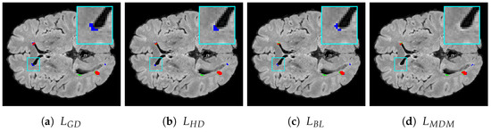
Figure 6. Segmentation results for the ISBI-MS dataset: (a) generalized Dice loss, (b) Hausdorff distance loss, (c) boundary loss, (d) Mahalanobis distance loss with $\lambda =1.5$. True positives, false negatives, and false positives are presented as red, green, and blue voxels, respectively. A representative RoI is zoomed in on for improved visualization, where the ground-truth and model prediction contours are overlaid in red and blue, respectively, for visual comparison.

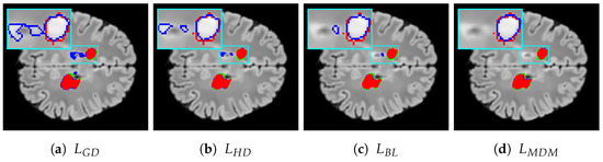
Figure 7. Segmentation results for the MSEEG2016 dataset: (a) generalized Dice loss, (b) Hausdorff distance loss, (c) boundary loss, (d) Mahalanobis distance loss with $\lambda =1.5$. True positives, false negatives, and false positives are presented as red, green, and blue voxels, respectively. A representative RoI is zoomed in on for improved visualization, where the ground-truth and model prediction contours are overlaid in red and blue, respectively, for visual comparison.

Voxels that are red denote true positives, green signifies false negatives, and blue indicates false positives. The figures for both datasets reveal that using the Mahalanobis distance loss leads to a reduction in the number of false positive errors and shows effective performance in minimizing false negatives. Specifically, when considering false positives, our loss function not only decreases the number of such voxels but also finds fewer false lesions, i.e., areas identified as lesions that are not actually present in the ground truth G. Regarding boundary distance metrics, it is clear that our loss function reduces the number of misclassified voxels not only near lesion boundaries but also further away from them, including false lesions.

5. Discussion

This work highlights the significant impact of selecting an effective loss function on segmenting multiple sclerosis lesions from MRI datasets. It evaluates various loss functions on the ISBI-MS and MSSEG datasets, noting that functions integrating spatial distance metrics, such as the Mahalanobis distance loss, surpass conventional overlap-based losses in boundary precision and segmentation accuracy. The Mahalanobis distance loss excels by achieving a compromise between clear boundary definition and high overall quality, while minimizing false positives and ensuring accurate lesion measurement.

The results obtained highlight the significance of empirically adjusting the Mahalanobis distance loss parameter to achieve optimal outcomes, with the results remaining consistent across various datasets, thus demonstrating robustness and generalizability. We recommend additional research focused on improving the recall and refining the loss functions, with our findings pointing to the Mahalanobis distance loss as a promising avenue for advancing MS lesion segmentation in clinical applications. Nonetheless, the Mahalanobis distance loss shows a tendency to favor precision over recall. This behavior can be explained by its penalty structure, where the Mahalanobis distance map assigns higher dissimilarity weights to background voxels near lesion boundaries than to lesion voxels near the background. Since MS lesions are small and more homogeneous than the background, the feature vectors of voxels inside lesions tend to be closer to the background prototype than background voxels are to the lesion prototype. As a result, false negatives within lesions receive milder penalties, whereas false positives in the heterogeneous background are penalized more severely. The exponent $\lambda$ plays a central role in this trade-off. Intermediate values of $\lambda$ provide the best balance between recall and precision, while very low or very high values shift the optimization toward one side of the trade-off at the expense of the other. Consequently, the Mahalanobis distance loss prioritizes the reduction of false positives and consistently achieves higher precision at the expense of slightly lower recall compared to region-based losses.

A concrete Dice score improvement from 0.7158 to 0.7247 and a reduction in HD95 from 30.29 mm to 27.02 mm on the ISBI-MS dataset, as demonstrated in this work, indicate more reliable lesion quantification and the earlier detection of disease progression in multiple sclerosis. These measurable advances provide clinicians with greater confidence for treatment adjustments and the definition of research endpoints for MS monitoring. Even moderate improvements in Dice (overall segmentation accuracy) and HD95 (boundary precision), as reported in our experiments, result in fewer missed or falsely labeled lesions, directly enhancing the accuracy and utility of clinical decision-making.

The principle limitations of the proposed Mahalanobis distance map method stem from its dependency on reliable covariance matrix estimation and texture feature extraction, which may become unstable in cases with very few boundary voxels, encountered in small or irregular MS lesions. Additionally, the method’s performance may be influenced by the quality and consistency of MRI acquisition and preprocessing, as radiomic texture features are sensitive to inter-patient and inter-scanner variability. Another important consideration is the observed trade-off between precision and recall: while the approach effectively reduces false positives, it can sometimes miss true lesion voxels, particularly for subtle or small lesions, suggesting reduced recall compared to standard overlap-based loss functions. Finally, although the computational overhead is generally manageable, expansion to diverse lesion types or modalities demands further validation to confirm its generalizability and robustness in varied clinical scenarios.

Regarding computational considerations, the Mahalanobis distance map entails a higher preprocessing cost, averaging approximately 24.9 min per volume. However, this step is performed only once and the resulting maps can be stored and reused across experimental runs. When the precomputed maps are simply loaded at the start of training, the effective computational cost and training time of using the Mahalanobis distance loss become essentially equivalent to those of the boundary loss. For example, training on the ISBI-MS dataset required about 27.9 s per epoch, showing no significant overhead compared with the boundary loss. Furthermore, during prediction, the network efficiency and resource usage are identical across loss functions, since segmentation is performed by the same CNN architecture and does not involve the loss function itself.

6. Conclusions

In this work, we introduce an innovative loss function, termed the Mahalanobis distance loss, designed for segmenting multiple sclerosis lesions in brain MRI scans. Distinct from conventional loss functions that depend merely on Euclidean distances, our method integrates local radiomic texture features in addition to the coordinates of each voxel. While a Euclidean distance assumes independence between variables and uses only coordinates to create a DTM, our approach leverages these features via the Mahalanobis distance map. This integration allows for the capture of pertinent subtleties around the lesion boundaries and extends the concepts of the DTM and SDF distance maps.

The findings reveal that the Mahalanobis-based loss function generally outperforms other existing loss functions across the assessed metrics. This implies that incorporating radiomic texture features into penalty calculations enhances distinction in uncertain regions, particularly where intensity overlaps arise from partial volume effects. Even in scenarios where the proposed method did not secure the top result, it maintained competitiveness, evidencing its robustness and stability.

An important point is that the computational cost of training with the Mahalanobis distance loss is equivalent to that of the boundary loss, owing to the fact that the distance map is calculated just once prior to training. This contrasts with other methods that require costly computations at every iteration. Additionally, in contrast to variants such as the active boundary loss, conditional boundary loss, and boundary-sensitive loss, which are limited to 2D images, our loss function is applicable to both 2D images and 3D volumes, enhancing its utility in volumetric MRI research.

In our future work, we intend to integrate more MRI acquisition channels into the Mahalanobis distance map, especially the T1-w modality, to better capture textures related to chronic lesions. Our goal is also to enhance the recall metric by decreasing false negatives while maintaining precision. We will also aim to improve specific metrics such as the lesion false positive rate and lesion false negative rate. Furthermore, we plan to accelerate the computation of the Mahalanobis distance map by employing parallelization strategies, enabling more efficient processing of high-dimensional MRI data. Another important direction is to evaluate the performance of the proposed loss function in segmenting other forms of brain lesions, such as tumors and vascular hyperintensities, as well as in abdominal organ medical images. Lastly, we plan to test the incorporation of the loss function into more sophisticated convolutional neural networks, such as Attention-UNet [42], or Transformer-based architectures to understand its impact on various medical segmentation tasks.

References

- Dobson, R.; Giovannoni, G. Multiple sclerosis—A review. Eur. J. Neurol. 2019, 26, 27–40. [Google Scholar] [CrossRef]
- Olejnik, P.; Roszkowska, Z.; Adamus, S.; Kasarełło, K. Multiple sclerosis: A narrative overview of current pharmacotherapies and emerging treatment prospects. Pharmacol. Rep. 2024, 76, 926–943. [Google Scholar] [CrossRef] [PubMed]
- Giorgio, A.; Stefano, N.D. Effective Utilization of MRI in the Diagnosis and Management of Multiple Sclerosis. Neurol. Clin. 2018, 36, 27–34. [Google Scholar] [CrossRef] [PubMed]
- Zhou, T.; Ruan, S.; Canu, S. A review: Deep learning for medical image segmentation using multi-modality fusion. Array 2019, 3–4, 100004. [Google Scholar] [CrossRef]
- Egger, C.; Opfer, R.; Wang, C.; Kepp, T.; Sormani, M.P.; Spies, L.; Barnett, M.; Schippling, S. MRI FLAIR lesion segmentation in multiple sclerosis: Does automated segmentation hold up with manual annotation? NeuroImage Clin. 2017, 13, 264–270. [Google Scholar] [CrossRef]
- Naga Karthik, E.; McGinnis, J.; Wurm, R.; Ruehling, S.; Graf, R.; Valosek, J.; Benveniste, P.L.; Lauerer, M.; Talbott, J.; Bakshi, R.; et al. Automatic segmentation of spinal cord lesions in MS: A robust tool for axial T2-weighted MRI scans. Imaging Neurosci. 2025, 3, IMAG.a.45. [Google Scholar] [CrossRef]
- Basaran, B.; Matthews, P.; Bai, W. New lesion segmentation for multiple sclerosis brain images with imaging and lesion-aware augmentation. Front. Neurosci. 2022, 16, 1007453. [Google Scholar] [CrossRef]
- Freire, P.G.L.; Ferrari, R.J. Multiple sclerosis lesion enhancement and white matter region estimation using hyperintensities in FLAIR images. arXiv 2018, arXiv:1807.09619. [Google Scholar] [CrossRef]
- Spagnolo, F.; Depeursinge, A.; Schädelin, S.; Akbulut, A.; Müller, H.; Barakovic, M.; Melie-Garcia, L.; Bach Cuadra, M.; Granziera, C. How far MS lesion detection and segmentation are integrated into the clinical workflow? A systematic review. NeuroImage Clin. 2023, 39, 103491. [Google Scholar] [CrossRef]
- Danelakis, A.; Theoharis, T.; Verganelakis, D.A. Survey of automated multiple sclerosis lesion segmentation techniques on magnetic resonance imaging. Comput. Med. Imaging Graph. 2018, 70, 83–100. [Google Scholar] [CrossRef]
- Birenbaum, A.; Greenspan, H. Multi-view longitudinal CNN for multiple sclerosis lesion segmentation. Eng. Appl. Artif. Intell. 2017, 65, 111–118. [Google Scholar] [CrossRef]
- Valverde, S.; Cabezas, M.; Roura, E.; González-Villà, S.; Pareto, D.; Vilanova, J.C.; Ramió-Torrentà, L.; Àlex, R.; Oliver, A.; Lladó, X. Improving automated multiple sclerosis lesion segmentation with a cascaded 3D convolutional neural network approach. NeuroImage 2017, 155, 159–168. [Google Scholar] [CrossRef]
- Belwal, P.; Singh, S. Deep Learning techniques to detect and analysis of multiple sclerosis through MRI: A systematic literature review. Comput. Biol. Med. 2025, 185, 109530. [Google Scholar] [CrossRef] [PubMed]
- Azad, R.; Aghdam, E.K.; Rauland, A.; Jia, Y.; Avval, A.H.; Bozorgpour, A.; Karimijafarbigloo, S.; Cohen, J.P.; Adeli, E.; Merhof, D. Medical Image Segmentation Review: The Success of U-Net. IEEE Trans. Pattern Anal. Mach. Intell. 2024, 46, 10076–10095. [Google Scholar] [CrossRef] [PubMed]
- Ronneberger, O.; Fischer, P.; Brox, T. U-Net: Convolutional Networks for Biomedical Image Segmentation. In Proceedings of the Medical Image Computing and Computer-Assisted Intervention—MICCAI 2015, Munich, Germany, 5–9 October 2015; Navab, N., Hornegger, J., Wells, W.M., Frangi, A.F., Eds.; Springer: Cham, Switzerland, 2015; pp. 234–241. [Google Scholar]
- Gallardo, C.A.Z.; Herrera, M.F.G.; Acosta, A.V.; Flores, D.A.M.; Santos, O.A.V.; Avalos, J.M.S.; del Carmen Perez Careta, M.; Careta, E.P. 3D Multiple Sclerosis Image Analysis Based on Probabilistic Methods for a 4F Array. In Proceedings of the Frontiers in Optics/Laser Science, Washington, DC, USA, 16–20 September 2018; Optica Publishing Group: Washington, DC, USA, 2018; p. JTu2A.139. [Google Scholar] [CrossRef]
- Yılmaz Acar, Z.; Başçiftçi, F.; Ekmekci, A.H. A Convolutional Neural Network model for identifying Multiple Sclerosis on brain FLAIR MRI. Sustain. Comput. Inform. Syst. 2022, 35, 100706. [Google Scholar] [CrossRef]
- Yılmaz Acar, Z.; Başçiftçi, F.; Ekmekci, A.H. Future activity prediction of multiple sclerosis with 3D MRI using 3D discrete wavelet transform. Biomed. Signal Process. Control 2022, 78, 103940. [Google Scholar] [CrossRef]
- Sudre, C.H.; Li, W.; Vercauteren, T.; Ourselin, S.; Cardoso, M.J. Generalised Dice Overlap as a Deep Learning Loss Function for Highly Unbalanced Segmentations. In Deep Learning in Medical Image Analysis and Multimodal Learning for Clinical Decision Support; Springer: Cham, Switzerland, 2017; Volume 2017, pp. 240–248. [Google Scholar] [CrossRef]
- Karimi, D.; Salcudean, S.E. Reducing the Hausdorff Distance in Medical Image Segmentation With Convolutional Neural Networks. IEEE Trans. Med. Imaging 2020, 39, 499–513. [Google Scholar] [CrossRef]
- Ma, J.; Wei, Z.; Zhang, Y.; Wang, Y.; Lv, R.; Zhu, C.; Chen, G.; Liu, J.; Peng, C.; Wang, L.; et al. How Distance Transform Maps Boost Segmentation CNNs: An Empirical Study. In Proceedings of the Medical Imaging with Deep Learning, Montreal, QC, Canada, 6–8 July 2020; Arbel, T., Ayed, I.B., de Bruijne, M., Descoteaux, M., Lombaert, H., Pal, C., Eds.; PMLR: Breckenridge, CO, USA, 2020; Volume 121, pp. 479–492. [Google Scholar]
- Kervadec, H.; Bouchtiba, J.; Desrosiers, C.; Granger, E.; Dolz, J.; Ben Ayed, I. Boundary loss for highly unbalanced segmentation. Med. Image Anal. 2021, 67, 101851. [Google Scholar] [CrossRef]
- Wang, C.; Zhang, Y.; Cui, M.; Liu, J.; Ren, P.; Yang, Y.; Xie, X.; Hua, X.; Bao, H.; Xu, W. Active Boundary Loss for Semantic Segmentation. In Proceedings of the AAAI Conference on Artificial Intelligence, Virtual, 11–15 October 2021. [Google Scholar]
- Mayerhoefer, M.; Materka, A.; Langs, G.; Häggström, I.; Szczypiński, P.; Gibbs, P.; Cook, G. Introduction to Radiomics. J. Nucl. Med. 2020, 4, 488–495. [Google Scholar] [CrossRef]
- Friedman, J.; Hastie, T.; Tibshirani, R. Sparse inverse covariance estimation with the graphical LASSO. Biostatistics 2008, 9, 432–441. [Google Scholar] [CrossRef]
- Frery, A.C.; Perciano, T. Introduction to Image Processing Using R: Learning by Examples; Springer: Cham, Switzerland, 2013. [Google Scholar]
- Hashemi, S.R.; Mohseni Salehi, S.S.; Erdogmus, D.; Prabhu, S.P.; Warfield, S.K.; Gholipour, A. Asymmetric Loss Functions and Deep Densely-Connected Networks for Highly-Imbalanced Medical Image Segmentation: Application to Multiple Sclerosis Lesion Detection. IEEE Access 2019, 7, 1721–1735. [Google Scholar] [CrossRef]
- Jadon, S. A survey of loss functions for semantic segmentation. In Proceedings of the 2020 IEEE Conference on Computational Intelligence in Bioinformatics and Computational Biology (CIBCB), Viña del Mar, Chile, 27–29 October 2020; pp. 1–7. [Google Scholar] [CrossRef]
- Yi-de, M.; Qing, L.; Zhi-bai, Q. Automated image segmentation using improved PCNN model based on cross-entropy. In Proceedings of the 2004 International Symposium on Intelligent Multimedia, Video and Speech Processing, Hong Kong, China, 20–22 October 2004; pp. 743–746. [Google Scholar] [CrossRef]
- Milletari, F.; Navab, N.; Ahmadi, S.A. V-Net: Fully Convolutional Neural Networks for Volumetric Medical Image Segmentation. In Proceedings of the 2016 Fourth International Conference on 3D Vision (3DV), Stanford, CA, USA, 25–28 October 2016; pp. 565–571. [Google Scholar] [CrossRef]
- Du, J.; Guan, K.; Liu, P.; Li, Y.; Wang, T. Boundary-Sensitive Loss Function With Location Constraint for Hard Region Segmentation. IEEE J. Biomed. Health Inform. 2023, 27, 992–1003. [Google Scholar] [CrossRef] [PubMed]
- Wu, D.; Guo, Z.; Li, A.; Yu, C.; Gao, C.; Sang, N. Conditional Boundary Loss for Semantic Segmentation. IEEE Trans. Image Process. 2023, 32, 3717–3731. [Google Scholar] [CrossRef] [PubMed]
- Varmuza, K.; Filzmoser, P. Introduction to Multivariate Statistical Analysis in Chemometrics, 1st ed.; Academic Press: Cambridge, MA, USA, 2009. [Google Scholar]
- Haralick, R.M.; Shanmugam, K.; Dinstein, I. Textural Features for Image Classification. IEEE Trans. Syst. Man Cybern. 1973, SMC-3, 610–621. [Google Scholar] [CrossRef]
- Galloway, M.M. Texture analysis using gray level run lengths. Comput. Graph. Image Process. 1975, 4, 172–179. [Google Scholar] [CrossRef]
- Carass, A.; Roy, S.; Jog, A.; Cuzzocreo, J.L.; Magrath, E.; Gherman, A.; Button, J.; Nguyen, J.; Prados, F.; Sudre, C.H.; et al. Longitudinal multiple sclerosis lesion segmentation: Resource and challenge. NeuroImage 2017, 148, 77–102. [Google Scholar] [CrossRef]
- Commowick, O.; Istace, A.; Kain, M.; Laurent, B.; Leray, F.; Simon, M.; Pop, S.C.; Girard, P.; Améli, R.; Ferré, J.C.; et al. Objective Evaluation of Multiple Sclerosis Lesion Segmentation using a Data Management and Processing Infrastructure. Sci. Rep. 2018, 8, 13650. [Google Scholar] [CrossRef]
- Jenkinson, M.; Beckmann, C.F.; Behrens, T.E.; Woolrich, M.W.; Smith, S.M. FSL. NeuroImage 2012, 62, 782–790. [Google Scholar] [CrossRef]
- Ansel, J.; Yang, E.; He, H.; Gimelshein, N.; Jain, A.; Voznesensky, M.; Bao, B.; Bell, P.; Berard, D.; Burovski, E.; et al. PyTorch 2: Faster Machine Learning Through Dynamic Python Bytecode Transformation and Graph Compilation. In Proceedings of the 29th ACM International Conference on Architectural Support for Programming Languages and Operating Systems (ASPLOS ’24), San Diego, CA, USA, 27 April–1 May 2024; Association for Computing Machinery: New York, NY, USA, 2024; Volume 2, pp. 929–947. [Google Scholar] [CrossRef]
- Cruz, P.; Ulloa, G.; Martín, D.S.; Veloz, A. Software Architecture Evaluation of a Machine Learning Enabled System: A Case Study. In Proceedings of the 2023 42nd IEEE International Conference of the Chilean Computer Science Society (SCCC), Concepción, Chile, 23–26 October 2023; pp. 1–8. [Google Scholar] [CrossRef]
- Nai, Y.H.; Teo, B.W.; Tan, N.L.; O’Doherty, S.; Stephenson, M.C.; Thian, Y.L.; Chiong, E.; Reilhac, A. Comparison of metrics for the evaluation of medical segmentations using prostate MRI dataset. Comput. Biol. Med. 2021, 134, 104497. [Google Scholar] [CrossRef]
- Oktay, O.; Schlemper, J.; Folgoc, L.L.; Lee, M.; Heinrich, M.; Misawa, K.; Mori, K.; McDonagh, S.; Hammerla, N.Y.; Kainz, B.; et al. Attention U-Net: Learning Where to Look for the Pancreas. arXiv 2018, arXiv:1804.03999. [Google Scholar] [CrossRef]
Disclaimer/Publisher’s Note: The statements, opinions and data contained in all publications are solely those of the individual author(s) and contributor(s) and not of MDPI and/or the editor(s). MDPI and/or the editor(s) disclaim responsibility for any injury to people or property resulting from any ideas, methods, instructions or products referred to in the content. |
© 2025 by the authors. Licensee MDPI, Basel, Switzerland. This article is an open access article distributed under the terms and conditions of the Creative Commons Attribution (CC BY) license (https://creativecommons.org/licenses/by/4.0/).