Adhesion Control of High-Speed Train Based on Improved Nonlinear Kalman Filter

Abstract

In the operation of high-speed trains, the effective transmission of traction force heavily relies on the adhesion between the wheel and the rail. Excessive traction or braking force may exceed the adhesion limit, causing wheel creep or slide, which threatens both equipment and safety. To address this, a state estimation method based on the SVD-ACKF (singular value decomposition adaptive cubature Kalman filter) is proposed for high-precision estimation of train speed. Combined with an extremum-seeking algorithm, a closed-loop adhesion control strategy is developed to maintain train operations near the maximum adhesion point. Simulation results show that the method ensures accurate tracking under varying rail conditions and noise, while the control algorithm maintains adhesion utilization above 90%, thereby meeting operational demands and enhancing railway safety.

1. Introduction

The utilization rate of adhesion between the wheel and rail not only restricts the traction performance of the train but also significantly impacts the safety and stability of train operation. Adhesion is influenced by various factors, such as rail surface conditions and operating conditions [1,2], and the high-speed operation of high-speed trains places higher demands on the efficient and stable utilization of adhesion. In the train traction control system, the traction coefficient decreases with an increase in the slip ratio [3,4]; thus, maximizing the utilization of adhesion between the wheel and rail is particularly crucial.

The traditional method for obtaining creep velocity involves acquiring accurate wheel speed information via wheel speed sensors, then using the minimum value of trailer wheel speed or multi-axis wheel speed to approximate train speed, and finally deriving the creep velocity. However, in practical applications, this method—using the minimum value as vehicle speed—introduces errors. To address this issue, this paper proposes a state estimation algorithm based on Singular Value Decomposition-Adaptive Cubature Kalman Filter (SVD-ACKF) for the high-precision estimation of train speed and adhesion coefficient. Previously, Y. Tao et al. [5] proposed an outlier-robust iterative extended Kalman filter (OR-IEKF) framework in the field of state estimation for nonlinear systems with outliers.

In the field of state estimation, numerous related studies have been conducted. For example, Reference [6] achieves train state estimation using the Unscented Kalman Filter (UKF) and provides the results to the torque controller to achieve maximum adhesion; Tian et al. [7] employs the Extended Kalman Filter (EKF) to achieve state estimation, applies it to adhesion control, and this method also provides an effective reference for obtaining important vehicle state parameters at low cost in the field of automotive adhesion control [8]; Huang et al. [9] proposes a joint filtering technique based on the Extended Kalman Filter (EKF) and Unscented Kalman Filter (UKF) to estimate the sideslip angle and road friction coefficient. In addition, Sun et al. [10] proposes a torque differential control method for dual rear-wheel hub motor drive systems based on vehicle state parameter estimation; Bertipaglia et al. [11] introduce Convolutional Neural Networks (CNN) into the Unscented Kalman Filter (UKF) for estimating the vehicle sideslip angle; Pichlík et al. [12] proposes a novel phase-shift detection method for slip controllers based on the Unscented Kalman Filter (UKF); Kobelski et al. [13] performs online estimation of traction parameters using the Adaptive Kalman Filter (AKF). Ji et al. [14] designs a peak adhesion coefficient observer and a yaw angle state observer for joint estimation. As a fundamental method for estimating the state of dynamic systems, Kalman filtering and smoothing techniques are also widely used in sensor networks [15,16], global satellite navigation and control systems [17,18], waterway tracking navigation systems [19], unmanned aerial vehicle attitude correction systems [20], and other fields. The EKF-DT system effectively addresses the limitations of EKF in high-altitude trajectory prediction by combining the optimized decision tree (DT) algorithm with the classical EKF and leveraging DT’s strong fitting ability for nonlinear data [21]. However, these studies face challenges in solving the Jacobian matrix or verifying the positive definiteness of the matrix in the actual model.

In the realm of control algorithms, the stick–slip problem has long been a focus of attention for vehicle dynamics researchers due to its significance in the railway field, and the rapid detection of stick–slip is a key area of traction control research [22,23]. He et al. [24] designs an adhesion control method based on the sliding mode extremum seeking for heavy-haul trains; in the field of automotive adhesion control, some studies have proposed a strategy based on Adaptive Sliding Mode Control (ASMC) to enhance path tracking accuracy under complex operating conditions [25]; Cheng et al. [26] proposes an improved algorithm based on UKF for fault detection in high-speed trains; Hu et al. [27] proposes using a low-pass filter to suppress sliding mode chattering, thereby reducing the limitations of fixed preview time in trajectory tracking; Fang et al. [28] proposes an adhesion control strategy based on wheel–rail adhesion state observation, which achieves improved adhesion control by establishing a single-axis dynamic model of high-speed trains, using a full-dimensional observer to monitor the wheel–rail tangential force coefficient, and adopting a recursive least squares method with a forgetting factor to predict the slope of the adhesion–creep curve; Liu et al. [29] designs an enhanced sliding mode controller to control and regulate the motor torque of heavy-haul trains. However, these control algorithms suffer from slow convergence speeds or large steady-state oscillations, highlighting the urgent need for a more effective control algorithm.

Based on the above analysis, this paper addresses the limitations of existing control algorithms—specifically convergence speed and steady-state oscillation—by proposing a train state estimation method based on an improved Kalman filter algorithm. This method employs the SVD-ACKF algorithm to achieve high-precision estimation of train speed and adhesion coefficient and integrates the sliding mode extremum-seeking algorithm to design an optimized adhesion control strategy. The goal is to enable the train to achieve a high adhesion utilization rate under different rail surface conditions and ensure its efficient and safe operation.

In summary, this study is organized as follows. Section 2 establishes the fundamental adhesion system models, including the wheel–rail adhesion model and the overall train dynamics. Section 3 develops the proposed SVD-ACKF algorithm for vehicle speed estimation, addressing the positive-definiteness issue of the covariance matrix. Section 4 validates the algorithm and control strategy through MATLAB/Simulink simulations and hardware-in-the-loop experiments under varying rail conditions. Finally, Section 5 summarizes the findings, highlights the advantages of the proposed method, and discusses its potential application value in high-speed train adhesion control.

2. Adhesion System Model

Wheel–rail adhesion is a complex nonlinear process influenced by various factors, including rail surface conditions (e.g., dry or wet states), wheel–rail contact stress, and relative creep velocity. To systematically characterize the wheel–rail adhesion mechanism and provide a theoretical foundation for subsequent adhesion control, this section is divided into two sections, where two core sub-models of the adhesion system are established. The details are as follows: First, grounded in the Hertz contact theory, this section analyzes the microscopic interaction mechanism between the wheel and rail. It clarifies the structural characteristics of the wheel–rail contact patch (including the adhesion zone and sliding zone) and defines key parameters associated with wheel–rail adhesion, such as creep velocity and adhesion coefficient. Subsequently, taking a typical four-motor four-trailer train as the research subject, this section simplifies the train dynamic model (e.g., by equating the frame-controlled biaxial model to a uniaxial model for mathematical tractability). On this basis, it derives the kinematic equations of the wheelset and the train’s overall dynamic equation. Additionally, influencing factors such as wind resistance are incorporated into the model, which lays a foundation for quantifying the effects of traction torque and external loads on wheel–rail adhesion.

2.1. Wheel–Rail Adhesion Model

The exertion of train traction depends on the adhesion between wheel and rail. The wheel–rail contact relationship is illustrated in Figure 1. When the train is running on the track, the contact area will undergo elastic deformation due to the effect of the wheel load $W\mathrm{g}$ at the contact between the wheel and the rail surface, forming an elliptical contact area. The contact area can be divided into two parts: adhesion area and sliding area. The adhesion area indicates that there is no relative sliding between wheel and rail in this area, while the sliding area indicates that there is relative sliding between wheel and rail in this area.

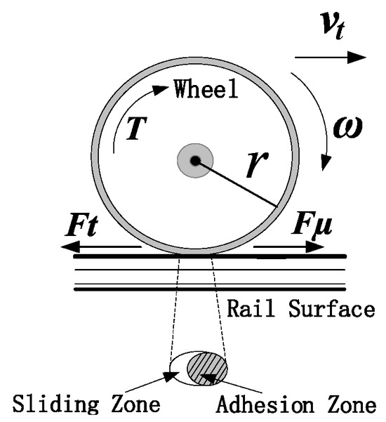
Figure 1. Wheel–rail contact relationship schematic.

According to the Hertz contact theory, during the operation of a train, due to the gravity of the car body acting on the track, the wheel–rail contact part will undergo elastic deformation. This deformation leads to the generation of contact stress between the wheel and rail, and results in an elliptical contact patch between them, as shown in Figure 1. The contact patch can be divided into two zones: the adhesion zone and the sliding zone. The adhesion zone refers to the area where no relative sliding occurs between the wheel and rail. Within this zone, there is a relatively high adhesion force between the wheel and rail, which enables the train to firmly adhere to the rail via this adhesion force and realize operations such as traction and braking. In contrast, the sliding zone is the area where slight relative sliding takes place between the wheel and rail. In this zone, due to incomplete contact conditions between the wheel and rail as well as the relative sliding between them, the adhesion force is relatively small while the sliding force is relatively large. The magnitude of the adhesion force determines the change in the areas of the contact patch zones. As the adhesion force increases, the adhesion zone shrinks, and the sliding zone expands. When the adhesion force increases to a certain critical value, the adhesion zone disappears, the wheel and rail enter a state of complete sliding, the adhesion state is destroyed, and the wheels start to spin. Therefore, the traction torque is limited by the maximum adhesion force on the rail surface, and the magnitude of the traction torque also drives changes in the adhesion on the rail surface.

The relative creep between the wheel and rail will cause the forward speed of the train to be less than the wheel circumference speed of the wheel. The difference between the two speeds is defined as the creep velocity $v_s$, and the expression is as follows:

$$v_s=\omega r-v_t$$

(1)

In the equation, r—wheel radius, ω—wheel angular velocity, v_t—train speed.

Under the action of traction torque $T$, the wheel will exert a force $F_T$ on the rail surface. According to the interaction of forces, the rail surface also produces a force $F_{\mu }$ on the wheel in the opposite direction of $F_T$, which is defined as the adhesion force between wheel and rail.

The adhesion coefficient $\mu$ between wheel and rail is defined as the ratio of the wheel–rail adhesion force $F_{\mu }$ to the vertical pressure of the train wheel axle load $W_g$ on the track, that is,

$$\mu =F_{\mu }/W_g$$

(2)

In view of the various influencing factors of the adhesion coefficient, although the O. Polach model takes into account the influence of various parameters, the formula is too complicated, and it is not practical to consider the functional research. Therefore, scholars have carried out many experimental analyses, summarized the relationship between the creep speed and the adhesion coefficient, and obtained the empirical formula model to describe the relationship between the two more simply.

The core formula is as follows [30,31]:

$$\mu =c\cdot e^{-a{v}_s}-d\cdot e^{-b{v}_s}$$

(3)

In the equation, a, b, c, d are parameters related to the rail surface; their values vary under different rail surface conditions and are summarized from numerous experiments. By setting the relevant parameters, the adhesion characteristic curves for these two common rail surfaces (dry rail surfaces and wet rail surfaces) can be obtained, as shown in Table 1 and Figure 2.

Table 1. Parameters for adhesion model under different rail surface conditions [32].

Rail Surface Conditions	a	b	c	d	The Maximum Adhesion Coefficient of the Current Rail Surface μmax
Dry rail surface	0.54	1.2	1	1	0.286
Wet rail surface	0.19	0.54	0.4	0.4	0.147

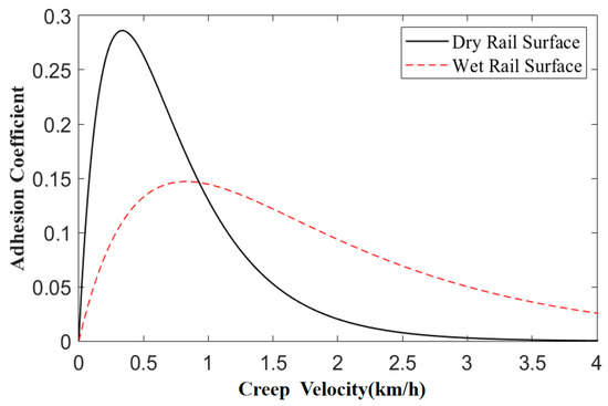
Figure 2. Adhesion characteristic curve.

In Figure 2 is the adhesion characteristic curve obtained by substituting the values in Table 1 into Equation (3). It can be seen from Figure 2 that although the adhesion characteristic curves of dry rail surface and wet rail surface are different, they all have similar changing trends, and there are adhesion peak points, which correspond to the maximum adhesion coefficient ${\mu }_{\max }$ in Table 1.

2.2. The Dynamic Model of the Train

Taking a four-motor four-trailer train as an example, the dynamic modeling of the train is carried out. A schematic diagram of the high-speed train set is presented in Figure 3. Among these, Carriages 1, 4, 5, and 8 are trailers, which are not equipped with power devices and do not undergo adhesion control. Carriages 2, 3, 6, and 7 are motor carriages, each employing a centralized electric control mode.

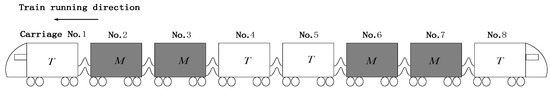
Figure 3. Diagram of a train.

In order to facilitate the analysis, in this paper, when conducting mathematical modeling, the frame control biaxial model is equivalent to the uniaxial model. Using this equivalent uniaxial model, the adhesion force of each power unit $F_{\mu }$ is

$$F_{\mu }=\mu Wg$$

(4)

According to the principle of dynamics, the kinematic equation of the wheelset in the above model is obtained as follows:

$$J_m{\displaystyle \frac{d{\omega }_m}{dt}}=T_m-T_L$$

(5)

$$T_L={\displaystyle \frac{F_u\cdot r}{R_g}}={\displaystyle \frac{\mu Wg\cdot r}{R_g}}$$

(6)

$$R_g={\displaystyle \frac{{\omega }_m}{{\omega }_d}}$$

(7)

$$v_d={\omega }_d\cdot r$$

(8)

Among them, $J_m$ is the rotational inertia of the traction motor; $T_m$—motor electromagnetic torque; $T_L$—load torque; ${\omega }_d$—wheel angular velocity; $v_d$—wheel line speed; ${\omega }_m$—angular velocity of traction motor; $R_g$—gear ratio; r—wheel radius.

According to the single-axis model in the overhead mode, the train shown in Figure 3 has four motor trains, four trailers, eight power bogies, sixteen moving shafts, and the train dynamics equation is

$${\displaystyle \sum _{i=1}^8{F}_{ui}-F_d}=(4M_M+4M_T){\displaystyle \frac{d{v}_t}{dt}}$$

(9)

Among them, $M_m$—motor vehicle quality; $M_T$—trailer quality; $F_d$—wind resistance during train operation is generally given by empirical equation, which is defined as

$$F_d=(27+0.0042v_t^2)\times (4M_M+4M_T)$$

(10)

3. SVD-ACKF Vehicle Speed Estimation Algorithm

The optimized adhesion control method focuses on how to maintain the maximum adhesion force during the train operation, that is, through the real-time optimization control strategy, to ensure that the train always runs near the adhesion peak point of the adhesion characteristic curve. To enhance the tracking speed and estimation accuracy in adhesion coefficient estimation, this paper employs the adaptive strong tracking filter (ASTF) algorithm. Subsequently, the adhesion coefficient estimated by adaptive strong tracking filter algorithm and the vehicle speed estimated by singular value decomposition adaptive cubature Kalman filter are fed into the adhesion controller.

The Kalman filtering algorithm includes three steps: initialization, prediction, and update. In the initialization phase, the initial state estimation and covariance matrix are set. In the prediction stage, the dynamic model of the system is used to predict the state estimation and covariance matrix of the next time. In the update phase, the predicted state is corrected using actual measurements via the measurement model.

Compared with the extended Kalman filter, the cubature Kalman filter introduces the spherical-radial cubature criterion in the prediction stage and uses a set of cubature points to approximate the state mean and covariance of the nonlinear system. With the increase in the number of Electric Multiple Units (EMUs), the information fusion between multiple vehicles and multiple axes leads to the increase in the state quantity of the vehicle speed estimation, which makes the dimension of the state-space equation increase, and the influence factors of unknown noise become significant. Therefore, this section designs an adaptive cubature Kalman filter algorithm based on singular value decomposition to estimate the vehicle speed.

3.1. Principle of the Cubature Kalman Filter Algorithm

The cubature criterion for CKF sampling mainly refers to the third-order spherical-radial cubature rule, and its principle is as follows: As known from the Bayesian recurrence formula, Bayesian filtering has theoretically achieved the optimal estimation of nonlinear filtering. However, to solve the nonlinear Gaussian filtering problem, it is necessary to address the difficulty in solving the integral of the product of multiple nonlinear functions and Gaussian density probability functions—and this is where the third-order spherical-radial cubature rule of CKF is proposed. First, the Gaussian integral of the system is transformed using cubature points into an n-dimensional spherical-radial integral form. The integral is then further decomposed into a spherical integral and a radial integral, and both are simplified. Based on this, the result of the spherical integral is substituted into the radial integral to obtain the third-order spherical-radial cubature rule approximation. Here, “third-order” indicates that all monomials up to the third order can be accurately approximated during this process, ensuring the accuracy of the CKF in nonlinear system state prediction and update.

Detailed derivation steps are as follows:

Assume the multi-dimensional weighted integral (i.e., the deformed complex integral) is as follows:

$$I\left(f\right)={\displaystyle {\int }_{R^n}f(x)\exp }(-x^{T}x)dx$$

(11)

For Equation (11), spherical-radial integral is used, and let $x=ry(r\in [0,\infty ],y\in R^n),y^{T}y=1$ be used for approximate transformation:

$$I\left(f\right)={\displaystyle \underset{0}{\overset{+\infty }{\int }}{\displaystyle {\int }_{U_n}f(ry)r^{n-1}\exp (-r^2)d\sigma (y)dr}}$$

(12)

where r is the radius of the sphere in spherical-radial coordinates, $U_n$ is unit spherical surface area, $U_n=\left\{y\in R^n\mid y_1^2+y_2^2+\cdots +y_n^2=1\right\}$, $\sigma$ is the spherical integral element of a sphere in spherical radial coordinates.

Decompose Equation (12) to obtain the spherical integral S(r) and radial integral I:

$$S(r)={\displaystyle {\int }_{U_n}f(ry)}d\sigma (y)$$

(13)

$$I={\displaystyle \underset{0}{\overset{\infty }{\int }}S}(r)r^{n-1}\exp (-r^2)dr$$

(14)

Approximate the radial integral I using the first-order Laguerre–Gauss quadrature formula:

$$I\approx {\displaystyle \frac{1}{2}}\Gamma ({\displaystyle \frac{n}{2}})S(\sqrt{{\displaystyle \frac{n}{2}}})$$

(15)

Approximate the spherical integral S(r) using the spherical cubature criterion:

$$S(r)\approx {\displaystyle \sum _{i=1}^{2n}{a}_i}f(r{s}_i)$$

(16)

where

$$\Gamma (n)={\displaystyle \underset{0}{\overset{+\infty }{\int }}{x}^{n+1}}\exp (-x)dx$$

(17)

$$s_i={[1]}_i$$

(18)

In the above, $\Gamma (n)$ is the Gamma function, and each cubature point $s_i$ has the same weight as $a_i$, and each weight is 1/(2n), leading to:

$$a_i={\displaystyle \frac{1}{2n}}{\displaystyle \frac{2\sqrt{{\pi }^n}}{\Gamma (n/2)}}$$

(19)

Based on the simplified radial integral in Equation (15) and spherical integral in Equation (16), the following is obtained:

$$I(f)\approx {\displaystyle \frac{\sqrt{{\pi }^n}}{2n}}{\displaystyle \sum _{i=1}^{2n}f}[\sqrt{{\displaystyle \frac{n}{2}}}{[1]}_i]$$

(20)

The above is the derivation process of the third-order spherical-radial cubature rule. Finally, combining it with the Gaussian distribution integral yields the third-order spherical-radial cubature rule in CKF, as shown in Equation (22).

For a standard Gaussian system, the following holds:

$$I_N\left(f\right)={\displaystyle {\int }_{R^n}f(x)N(x;0,I)dx\approx \frac{1}{\sqrt{{\pi }^n}}{\displaystyle {\int }_{R^n}f(\sqrt{2}x)}\exp }(-x^{\mathrm{T}}x)dx$$

(21)

Eventually, the spherical-radial cubature criterion is approximately expressed as

$$I_N(f)\approx {\displaystyle \frac{1}{\sqrt{{\pi }^n}}}({\displaystyle \frac{\sqrt{{\pi }^n}}{2n}}{\displaystyle \sum _{i=1}^{2n}f(\sqrt{2}\sqrt{\frac{n}{2}}{[1]}_i)})\approx {\displaystyle \sum _{i=1}^m{\omega }_{i}f}\left({\xi }_i\right)$$

(22)

where ${\xi }_i=\sqrt{m/2}{E}_i,{\omega }_i=1/m,(i=1,...,m,m=2n)$

As can be seen from the above analysis, to simplify the algorithm and reduce computational complexity, the CKF samples $m$ cubature points ($m=2n_x$, and $n_x$ is the system dimension) according to the third-order spherical-radial cubature rule and propagates these cubature points in the algorithm.

The flow of the CKF algorithm [33] is as follows:

Step 1: Initialization Stage

When k = 0, set the initial values of the state quantity $x_{0|0}$, state covariance matrix $P_{0|0}$, and noise covariance matrices Q and R.

Step 2: Prediction Stage, according to the third-order spherical-radial volume rule, the covariance matrix $P_{k|k}$ is decomposed by Cholesky, and ${\xi }_i$ is superimposed in each direction of the state variable to obtain $m$ volume points ${\chi }_i$, which are substituted into the state equation to realize the volume point propagation and obtain ${\chi }_i$. Finally, the state vector ${\widehat{x}}_{k+1|k}$ and the prediction quantity $P_{k+1|k}$ of the state error covariance matrix are obtained by weighted summation. The weight of each sampling point is $m$, $m=2n_x$, and $n_x$ is the system dimension.

Using the Cholesky decomposition method to decompose $P_{k|k}$ to obtain $S_{k|k}$

$$P_{k|k}=S_{k|k}{S}_{k|k}^T$$

(23)

Calculate the cubature points ${\chi }_i$ (i = 1, …, m) based on the decomposed results $S_{k|k}$:

$${\chi }_{i,k|k}=S_{k|k}{\xi }_i+{\widehat{x}}_{k|k}$$

(24)

where ${\xi }_i=\left\{\begin{array}{cc}{\sqrt{n}}_x{e}_i\hfill & i=1,2,...,2n_x\\ -\sqrt{n_x}{e}_i\hfill & i=n_x+1,n_x+2,...,2n_x\end{array}\right.$

Substitute ${\chi }_i$ into the state equation to obtain the propagated cubature points ${\chi }_i$:

$$X_{i,k+1|k}=f({\chi }_{i,k|k},u_k)$$

(25)

Calculate the predicted state vector ${\widehat{x}}_{k+1|k}$ and state error covariance matrix $P_{k+1|k}$ at the next moment $k+1$:

$${\widehat{x}}_{k+1|k}={\displaystyle \frac{1}{m}}{\displaystyle \sum _{i=1}^m{X}_{i,k+1|k}}$$

(26)

$$P_{k+1|k}={\displaystyle \frac{1}{m}}{\displaystyle \sum _{i=1}^m{X}_{i,k+1|k}}{X}_{i,k+1|k}^T-{\widehat{x}}_{k+1|k}{\widehat{x}}_{k+1|k}^T+Q$$

(27)

Step 3: Update Stage

Perform Cholesky decomposition on the predicted state error covariance matrix $P_{k+1|k}$ to obtain and propagate cubature points. Since the CKF uses cubature points to accurately approximate nonlinear functions, it involves the calculation of the innovation (measurement) covariance matrix $P_{yy,k+1|k}$ and cross-covariance matrix $P_{xy,k+1|k}$. Finally, update the Kalman gain $K_{k+1}$, state vector ${\widehat{x}}_{k+1|k+1}$, and error covariance matrix $P_{k+1|k+1}$ for subsequent algorithm iterations.

Perform Cholesky decomposition on $P_{k+1|k}$ to obtain the following:

$$P_{k+1|k}=S_{k+1|k}{S}_{k+1|k}^T$$

(28)

Calculate the cubature points ${\chi }_i$ (i = 1, …, 2)

$${\chi }_{i,k+1|k}=S_{k+1|k}{\xi }_i+{\widehat{x}}_{k+1|k}$$

(29)

Calculate the cubature points $Y_i$ propagated through the observation equation:

$$Y_{i,k+1|k}=h({\chi }_{i,k+1|k},u_k)$$

(30)

Calculate the output vector ${\widehat{y}}_{k+1|k}$ and innovation covariance matrix $P_{yy,k+1|k}$ at the next moment $k+1$:

$${\widehat{y}}_{k+1|k}={\displaystyle \frac{1}{m}}{\displaystyle \sum _{i=1}^m{Z}_{i,k+1|k}}$$

(31)

$$P_{yy,k+1|k}={\displaystyle \frac{1}{m}}{\displaystyle \sum _{i=1}^m{Y}_{i,k+1|k}{Y}_{i,k+1|k}^T}-{\widehat{y}}_{k+1|k}{\widehat{y}}_{k+1,k}^T+R$$

(32)

Predict the cross-covariance matrix $P_{xy,k+1|k}$ at the next moment $k+1$.

$$P_{xy,k+1|k}={\displaystyle \frac{1}{m}}{\displaystyle \sum _{i=1}^m{X}_{i,k+1|k}}{Y}_{i,k+1|k}^T-{\widehat{x}}_{k+1|k}{\widehat{y}}_{k+1,k}^T$$

(33)

Estimate the Kalman gain $K_{k+1}$:

$$K_{k+1}=P_{xy,k+1|k}{P}_{yy,k+1|k}^{-1}$$

(34)

Update the state vector ${\widehat{x}}_{k+1|k+1}$ at the next moment $k+1$:

$${\widehat{x}}_{k+1|k+1}={\widehat{x}}_{k+1|k}+K_{k+1}(y_{k+1}-{\widehat{y}}_{k+1|k})$$

(35)

Update the state error covariance matrix at the next moment:

$$P_{k+1|k+1}=P_{k+1|k}-K_{k+1}{P}_{yy,k+1|k}{K}_{k+1}^T$$

(36)

CKF calculates cubature points, propagates these points according to the system state equation, and performs data fusion using the weighted summation method—without the need to solve the Jacobian matrix of the state equation. Thus, it has a wider scope of application.

3.2. Principle of the SVD-ACKF Algorithm

As is analyzed in the principles of the CKF algorithm, both Equations (23) and (28) require Cholesky decomposition of the covariance matrix to select and propagate cubature points. However, in the actual train speed estimation process, the presence of external uncertain noise and the mutual fusion of sensor information among multi-vehicle and multi-axle systems can easily cause the covariance matrix to lose positive definiteness during the algorithm estimation process. Since matrix decomposition is required in each iteration of the CKF, this may lead to abnormal operation of the algorithm or even interruption of estimation.

Singular Value Decomposition is a matrix decomposition method with strong numerical stability and high accuracy. This section proposes the use of SVD to improve the stability of the CKF algorithm for system filter estimation [34].

SVD decomposes a matrix into the product of three matrices, in the form:

$$A=U\Sigma V^T$$

(37)

where $A$ is an m × n matrix, $U$ is an m × m orthogonal matrix, $\Sigma$ is an m × n diagonal matrix, and $V^T$ is an n × n orthogonal matrix. These three matrices represent the “left singular vectors”, “singular values”, and “right singular vectors” of the original matrix, respectively.

The covariance matrix can be expressed via SVD as follows:

$$P_k=U_k\left[\begin{array}{ll}{S}_k& 0\\ 0& 0\end{array}\right]V_k^T$$

(38)

In Equation (38), $S_k$ is a diagonal matrix and $S_k=diag[s_1,s_2...s_L]$.

The error covariance matrix is symmetric; thus, $U_k=V_k$ holds, where ${s_i}^2\left(i=1,2,\dots ,L\right)$ are the eigenvalues of $P_k$, and its eigenvectors are represented by the column vectors of $U{U}^T$.

After performing SVD on the error covariance matrix, Equation (28) is rewritten as

$$P_{k|k}=U_{k|k}{S}_{k|k}{V}_{k|k}^T$$

(39)

Calculate the cubature points:

$${\chi }_{i,k|k}=U_{i,k|k}\sqrt{S_{k|k}}{\xi }_i+{\widehat{x}}_{k|k}$$

(40)

Then, calculate the cubature points of the state equation and the predicted state and predicted variance using the same equations as before.

During the measurement update, Equation (28) needs to be rewritten as follows:

$$P_{k+1|k}=U_{k+1|k}{S}_{k+1|k}{V}_{k+1|k}^T$$

(41)

Calculate the cubature points:

$${\chi }_{i,k+1|k}=U_{i,k+|k}\sqrt{S_{k+1|k}}{\xi }_i+{\widehat{x}}_{k+1|k}$$

(42)

The subsequent steps are the same as those of the standard CKF.

Combining the CKF with adaptive filtering, the following update equations for the adaptive CKF are derived as presented in [35].

A weighting factor $d_{k+1}$ is introduced, along with a forgetting factor $b$ whose value lies between 0 and 1. The forgetting factor is empirically determined and is typically constrained within the interval [0.95, 0.99].

$$d_{k+1}=(1-b)/(1-b^{k+2})$$

(43)

Therefore, it can be regarded as an adaptive weighting coefficient based on the forgetting factor $b$. At the initial stage of filtering, the normalized form ensures a higher weight on new information, thereby accelerating convergence, whereas in the steady-state stage, it gradually converges to the constant $1-b$, ensuring the stability of the estimation.

The exponentially weighted update formula is as follows:

$${\widehat{\theta }}_{k+1}=\left(1-d_{k+1}\right){\widehat{\theta }}_k+d_{k+1}{\tilde{\theta }}_{k+1}$$

(44)

The exponential weighting approach is adopted, where ${\widehat{\theta }}_{k+1}$ denotes the recursively updated statistical estimate of the noise, and ${\widehat{\theta }}_{k+1}$ corresponds to the instantaneous estimate obtained from the data at time step k + 1.

Calculate the prediction covariance $P_{k+1\mid k}$ and the update covariance $P_{k+1\mid k+1}$ at the next moment k + 1.

$$P_{k+1\mid k}={\displaystyle \frac{1}{m}}{\displaystyle \sum _{i=1}^m{X}_{i,k+1\mid k}}{X}_{i,k+1\mid k}^T-{\widehat{x}}_{k+1\mid k}{\widehat{x}}_{k+1\mid k}^T+Q$$

(45)

$$P_{k+1\mid k+1}=P_{k+1\mid k}-K_{k+1}{S}_{k+1}{K}_{k+1}^T$$

(46)

where the empirical covariance of the residual is given by $e_{k+1}{e}_{k+1}^T\approx S_{k+1}$.

By subtracting the two expressions, the instantaneous estimate of the process noise covariance ${\tilde{Q}}_{k+1}$ at the next moment k + 1 is obtained.

$${\tilde{Q}}_{k+1}=K_{k+1}{e}_{k+1}{e}_{k+1}^T{K}_{k+1}^T+P_{k+1\mid k+1}-\left({\displaystyle \frac{1}{m}}{\displaystyle \sum _{i=1}^m{X}_{i,k+1\mid k}}{X}_{i,k+1\mid k}^T-{\widehat{x}}_{k+1\mid k}{\widehat{x}}_{k+1\mid k}^T\right)$$

(47)

Update the instantaneous estimate of the process noise mean ${\tilde{q}}_{k+1}$ at the next moment k + 1.

$${\tilde{q}}_{k+1}={\widehat{x}}_{k+1\mid k+1}-{\displaystyle \frac{1}{m}}{\displaystyle \sum _{i=1}^{m}f}\left({\widehat{x}}_{i,k+1\mid k},u_k\right)$$

(48)

Update the measurement noise $v_{k+1}$ and residual covariance $S_{k+1}$ at the next time step k + 1.

$$v_{k+1}=y_{k+1}-h\left(x_{k+1},u_k\right)$$

(49)

$$S_{k+1}={\displaystyle \frac{1}{m}}{\displaystyle \sum _{i=1}^m{Y}_{i,k+1\mid k}}{Y}_{i,k+1\mid k}^T-{\widehat{y}}_{k+1\mid k}{\widehat{y}}_{k+1\mid k}^T+R$$

(50)

Calculate the instantaneous estimate of the measurement noise covariance ${\tilde{R}}_{k+1}$ at the next moment k + 1.

$${\tilde{R}}_{k+1}=e_{k+1}{e}_{k+1}^T-\left({\displaystyle \frac{1}{m}}{\displaystyle \sum _{i=1}^m{Y}_{i,k+1\mid k}}{Y}_{i,k+1\mid k}^T-{\widehat{y}}_{k+1\mid k}{\widehat{y}}_{k+1\mid k}^T\right)$$

(51)

Update the instantaneous estimate of the measurement noise mean ${\tilde{r}}_{k+1}$ at the next moment k + 1.

$${\tilde{r}}_{k+1}=y_{k+1}-{\displaystyle \frac{1}{m}}{\displaystyle \sum _{i=1}^{m}h}\left({\widehat{x}}_{i,k+1\mid k},u_k\right)$$

(52)

Through derivation in accordance with Equation (44), the results are obtained, respectively.

$${\widehat{Q}}_{k+1}=(1-d_{k+1}){\widehat{Q}}_k+d_{k+1}\left[K_{k+1}{e}_{k+1}{e}_{k+1}^T{K}_{k+1}^T+P_{k+1|k+1}-({\displaystyle \frac{1}{m}}{\displaystyle \sum _{i=1}^m{X}_{i,k+1|k}}{X}_{i,k+1|k}^T-{\widehat{x}}_{k+1|k}{\widehat{x}}_{k+1|k}^T)\right]$$

(53)

$${\widehat{q}}_{k+1}=(1-d_{k+1}){\widehat{q}}_k+d_{k+1}({\widehat{x}}_{k+1|k+1}-{\displaystyle \frac{1}{m}}{\displaystyle \sum _{i=1}^{m}f({\widehat{x}}_{k+1|k},u_k)})$$

(54)

$${\widehat{R}}_{k+1}=(1-d_{k+1}){\widehat{R}}_k+d_{k+1}\left[e_{k+1}{e}_{k+1}^T-({\displaystyle \frac{1}{m}}{\displaystyle \sum _{i=1}^m{Y}_{i,k+1|k}{Y}_{i,k+1|k}^T}-{\widehat{y}}_{k+1|k}{\widehat{y}}_{k+1,k}^T)\right]$$

(55)

$${\widehat{r}}_{k+1}=(1-d_{k+1}){\widehat{R}}_k+d_{k+1}(y_{k+1}-{\displaystyle \frac{1}{m}}{\displaystyle \sum _{i=1}^{m}h({\widehat{x}}_{i,k+1|k},u_k)})$$

(56)

In cases where the system state dimension is high, estimation anomalies may occur, which in turn lead to algorithm filter divergence. This situation arises because $Q_k$ and $R_k$ change during iteration, resulting in the loss of semi-positive definiteness of $Q_k$ and positive definiteness of $R_k$. To prevent filter divergence and failure, a biased noise variance estimator is adopted for estimation:

$$Q_k=(1-d_k)Q_{k-1}+d_k\left[K_k{e}_k{e}_k^T{K}_k^T\right]$$

(57)

$$R_k=(1-d_k)R_{k-1}+d_k\left[e_k{e}_k^T\right]$$

(58)

When positive definiteness issues occur in $Q_k$ and $R_k$, Equations (57) and (58) are used to estimate $Q_k$ and $R_k$, while the $P_{k+1|k+1}-({\displaystyle \frac{1}{m}}{\displaystyle \sum _{i=1}^m{X}_{i,k+1|k}}{X}_{i,k+1|k}^T-{\widehat{x}}_{k+1|k}{\widehat{x}}_{k+1|k}^T)$ terms in Equation (53) and the $({\displaystyle \frac{1}{m}}{\displaystyle \sum _{i=1}^m{Y}_{i,k+1|k}{Y}_{i,k+1|k}^T}-{\widehat{y}}_{k+1|k}{\widehat{y}}_{k+1,k}^T)$ terms in Equation (55) are ignored. This ensures that $Q_k$ and $R_k$ maintain semi-positive definiteness and positive definiteness in real time during the filtering process.

Therefore, in the final adaptive update process, the corresponding equations are selected for update after judging ${\widehat{Q}}_k$ and ${\widehat{R}}_k$:

$${\widehat{Q}}_k=\left\{\begin{array}{ll}estimation {\widehat{Q}}_{k-1},& {\widehat{Q}}_k is a positive semi-definite matrix\\ (1-d_k){\widehat{Q}}_{k-1}+d_k\left[K_k{e}_k{e}_k^T{K}_k^T\right],& {\widehat{Q}}_k is not a positive semi-definite matrix\end{array}\right.$$

(59)

$${\widehat{R}}_k=\left\{\begin{array}{ll}estimation {\widehat{R}}_{k-1},& {\widehat{R}}_k is a positive semi-definite matrix\\ (1-d_k){\widehat{R}}_k+d_k\left[e_k{e}_k^T\right],& {\widehat{R}}_k is not a positive semi-definite matrix\end{array}\right.$$

(60)

The algorithm flow chart of the SVD-ACKF is shown in Figure 4.

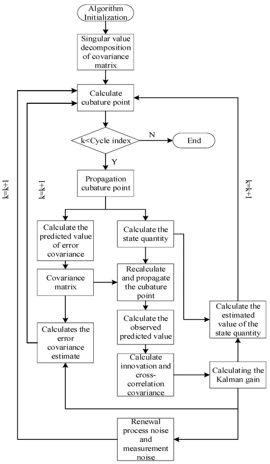
Figure 4. The flow chart of SVD-ACKF.

3.3. The HIL Simulation Platform and Experimental Design

The hardware-in-the-loop (HIL) simulation platform is mainly based on the MT PXI HIL real-time simulator developed by National Instruments, Austin, TX, USA (NI). It is mainly divided into two parts: hardware and software.

The platform mainly uses MATLAB/Simulink R2014a software and StarSim v4.6 host computer software. Simulink is used to build the offline simulation model, while StarSim host computer software connects the PC-side offline simulation model with the real-time simulator. The process is illustrated in Figure 5.

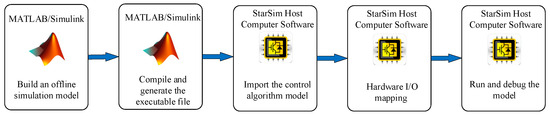
Figure 5. Software part.

The hardware components, including a high-speed I/O signal transfer board and a real-time simulator, are shown in Figure 6. The signal transfer board is used to transfer the output signals of the real-time simulator mainly through StarSim software and can also serve as an innovation interaction interface for HIL experiment signals. Internally, the real-time simulator mainly consists of a field-programmable gate array (FPGA) computing board and a multi-core CPU. The FPGA computing board is mainly designed for small-step simulation experiments; it has a fast-computing speed, reaching the level of 0.2~1.25 μs. The multi-core CPU is mainly used for large-step simulation experiments, with a computing step size of 25~100 μs. The combination of the two reflects the high-performance function of the real-time simulator. Both can load models, which effectively improves simulation efficiency.

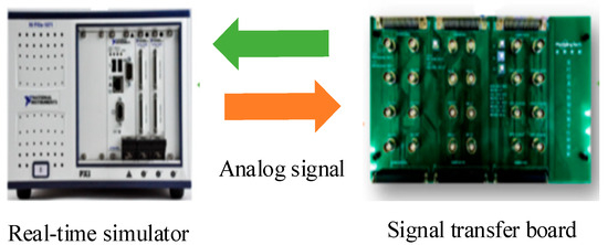
Figure 6. Hardware part.

The simulation model of a high-speed train is built in MATLAB/Simulink, and the verification experiment of the adhesion control method is based on the state estimation of high-speed train that is carried out by combining state estimation and adhesion control algorithm.

First, a train dynamics model is established. Considering the differences in adhesion conditions on different rail surfaces when EMUs are in operation, the adhesion coefficient estimated based on ASTF and the vehicle speed estimated based on SVD-ACKF are applied to the model. Through continuous dynamic adjustment, the extreme point of the current operating conditions (i.e., the adhesion peak point) is searched for; the obtained optimal creep speed under the corresponding operating conditions is then input into the backstepping controller, which in turn outputs the control torque to achieve optimized adhesion control. Finally, the real-time performance and effectiveness of the state estimation-based adhesion control algorithm are verified on the MT PXI HIL simulation platform developed by NI. The overall flow chart of adhesion control based on high-speed train state estimation is shown in Figure 7.

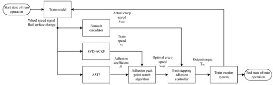
Figure 7. Train control flow chart.

4. Experiment and Analysis

The estimation of vehicle speed based on SVD-ACKF is designed. The relevant model is built in Matlab/Simulink. The train dynamics parameters are shown in Table 2, R_g = 3.036, r = 0.41 m, W = 13.5 t, M = 550 t, J = 55.3 kg·m². The Gaussian white noise is set as the interference signal in the adhesion characteristics, system state noise, and measurement noise.

Table 2. Train parameters.

Parameter	Numeric Value	Parameter	Numeric Value
M	550 × 103 kg	Rg	3.036
N	4	Jm	6 kg·m2
J	55.3 kg·m2	W	13.5 × 103 kg
r	0.41 m	G	9.8 m/s2

The algorithm parameter values are set as follows: the initial value of the state covariance matrix P₀ = 0.01I_5×5, the initial value of the state quantity x₀ = [0,0]^T, Q = 0.001I_5×5, R = 0.2I_4×4.

The process noise mainly comes from motor torque fluctuation, which is determined by the 2% fluctuation of the motor’s rated torque 6000 N·m. That is, $Q={(\Delta T_e/R_{g}r)}^2{I}_{5\times 5}=0.001I_{5\times 5}$, where $(\Delta T_e=120$$\mathrm{N}\cdot \mathrm{m})$. The observation noise comes from the wheel speed sensor and is determined by the sensor accuracy $\Delta \omega =0.01 \mathrm{rad}/\mathrm{s}$. That is, $R={(\Delta \omega \cdot r)}^2{I}_{4\times 4}=0.2I_{4\times 4}$.

The sampling time is set to T = 0.001, the running time is set to t = 70 s, and the adaptive forgetting factor is 0.95. In the adaptive CKF algorithm, Q, and R can be updated at the same time. At this time, the adhesion coefficient condition adopts the adhesion empirical model, and the dry rail surface coefficient is a = 0.54, b = 1.2, c = 1.0, d = 1.0.

To verify the effectiveness of the estimation algorithm, a special operating condition is designed as follows: a control torque value for the train in the system is artificially specified, and the wheelset idling of the train on different track surfaces is observed. Meanwhile, when the system input torque is given, Gaussian white noise interference is added as the input torque of the system, and the setting of the given torque is shown in Figure 8.

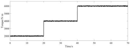
Figure 8. Artificially specified train control torque.

After the artificially specified train control torque is applied, the condition is illustrated in Figure 8. Considering the changes in track surface conditions during actual operation, two working scenarios—dry and wet rail surfaces—are set, and the resulting variation in output creep speed is illustrated in Figure 9. Under the influence of the current torque, different rail surfaces have experienced the destruction of the adhesion characteristics at different time points of a given torque change. Wheelset idling occurs when the wet rail surface t = 20 s. At this time, the adhesion coefficient of the motor vehicle is 0. Similarly, the wheelset idling occurs when the dry rail surface is t = 40 s.

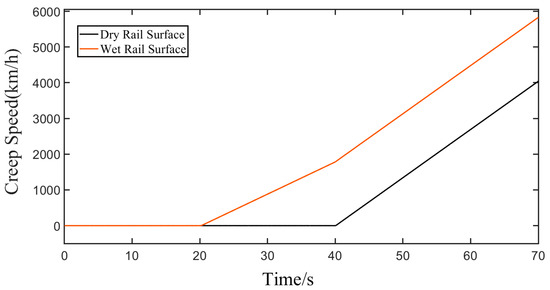
Figure 9. The creep speed output by two rail surfaces.

An optimized adhesion control method based on adhesion peak point search is designed, and the key adhesion parameters (adhesion coefficient and train speed) obtained by state estimation are used as input parameters of the adhesion control method. In order to verify the effectiveness of the algorithm, the white noise interference with a variance of 0.001 is added to the adhesion characteristics, and the white noise interference with a variance of 0.001 is superimposed on the speed sensor. This setting can effectively test the effectiveness of the estimation algorithm. At this time, the parameters are selected as Table 2.

Because the estimation effect of the adhesion coefficient of each vehicle is consistent, only the analysis of vehicle 1 is carried out at this time. For example, Figure 10c shows the actual adhesion coefficient of vehicle 1 and Figure 10d shows the estimated adhesion coefficient of unit 1. In order to obtain the effect of the estimation algorithm more realistically, white noise interference is directly superimposed on the adhesion characteristics, so the real adhesion coefficient fluctuates greatly at this time. Through comparative observation, it can be seen that the adhesion coefficient estimation method based on SVD-ACKF can track the change in the adhesion coefficient of the upper rail surface in real time and realize the filtering of Gaussian white noise interference.

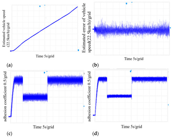
Figure 10. Estimated results of unit 1 under noisy conditions. (a) Estimated vehicle speed. (b) Estimated error of vehicle speed. (c) The actual adhesion coefficient of unit 1 (adding white noise). (d) The estimated adhesion coefficient of unit 1.

To demonstrate the effectiveness of the proposed adhesion control strategy, simulations were conducted under time-varying rail conditions: the rail surface was dry before 20 s, transitioned to wet from 20 s to 40 s, and reverted to dry after 40 s. The control output torque of unit 1 is presented in Figure 11, where the curves of SVD-ACKF (orange), CKF (green), UKF (blue), and the actual torque value (red) are compared.

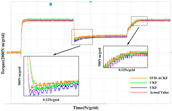
Figure 11. Comparison of SVD-ACKF, CKF, UKF and actual value for output torque.

At t = 0 s, the estimation algorithm and control method were activated. All algorithms responded to track the optimal adhesion torque. The SVD-ACKF curve rapidly converged to the actual torque with the smallest overshoot and oscillation: at t = 3 s (when the optimal adhesion point was identified), its torque amplitude reached only 2.25%. In contrast, CKF exhibited a torque amplitude of 8.14% (5.89% higher than SVD-ACKF), while UKF showed the largest amplitude (10.25%). This indicates that SVD-ACKF achieved superior transient stability and tracking precision compared to CKF and UKF during the initial identification phase.

When the rail surface became wet at t = 20 s, the adhesion characteristic changed, requiring the control system to adapt. As shown in the lower-left enlarged figure of Figure 11 (time scale: 0.125 s/grid), the SVD-ACKF torque curve closely followed the actual value with minimal deviation: its amplitude was 3.65%, which is 11.55% lower than CKF’s 15.2% and much closer to the actual torque. UKF had a torque amplitude of 12.7% (smaller than CKF but larger than SVD-ACKF), confirming that SVD-ACKF maintained better tracking accuracy under wet rail conditions.

After t = 40 s, when the rail surface returned to dry, as shown in the rightmost enlarged figure of Figure 11 (time scale: 0.125 s/grid), the amplitude of the SVD-ACKF torque curve was 2.1%, which is closest to the stable torque level. The amplitude of the CKF torque curve was 3.06%, showing moderate fluctuation. The oscillation amplitude of the UKF torque curve was the largest at 5.1%. This shows that SVD-ACKF had stronger anti-interference robustness during the transition back to dry rail conditions.

In summary, across all rail condition stages, SVD-ACKF outperformed CKF and UKF in terms of torque tracking precision, transient stability, and robustness against disturbances—as evidenced by its closer alignment with the actual torque and smaller amplitude deviations in Figure 11.

For the three algorithms, UKF, CKF, and SVD-ACKF, this study employs three performance metrics for comparison: root mean square error (RMSE), maximum estimation error, and convergence time, as summarized in Table 3.

Table 3. Performance comparison of UKF, CKF, and SVD-ACKF in terms of RMSE, maximum estimation error, and convergence time.

Algorithm	RMSE (%)	Max Error (%)	Convergence Time (s)
UKF	0.73	12.71	1.154
CKF	0.52	15.19	1.068
SVD-ACKF	0.31	6.56	1.013

The performance of the UKF, CKF, and SVD-ACKF in terms of RMSE, maximum estimation error, and convergence time is compared in Table 3. Among these metrics, RMSE represents the overall estimation accuracy. As can be seen from the table, the RMSE value of SVD-ACKF is 0.31%, which is the smallest among the three; followed by CKF with an RMSE value of 0.52%; the worst is UKF with an RMSE value of 0.73%, which is almost more than twice of SVD-ACKF. The maximum error reflects the deviation under the worst-case condition: the maximum error of CKF is 15.19%, followed by UKF at 12.71%, and SVD-ACKF performs the best with a maximum error of 6.56%. Convergence time is defined as the earliest moment when the relative error remains below 0.5% for at least 1 s. Among the three filters, SVD-ACKF achieves the fastest convergence with a time of 1.013 s, followed by CKF at 1.068 s, and finally UKF at 1.154 s. The results indicate that the maximum error mainly occurs during the first rail condition switching; thereafter, due to its faster response speed, SVD-ACKF achieves the shortest convergence time while maintaining the lowest overall RMSE, demonstrating its superiority in both accuracy and robustness.

To demonstrate the effectiveness of the proposed adhesion control strategy, simulations were conducted under time-varying rail conditions: the rail surface was dry before 20 s, transitioned to wet from 20 s to 40 s, and reverted to dry after 40 s. The train speed curve of unit 1 is presented in Figure 12, where the curves of SVD-ACKF (orange), CKF (green), UKF (blue), and the actual speed (red) are compared.

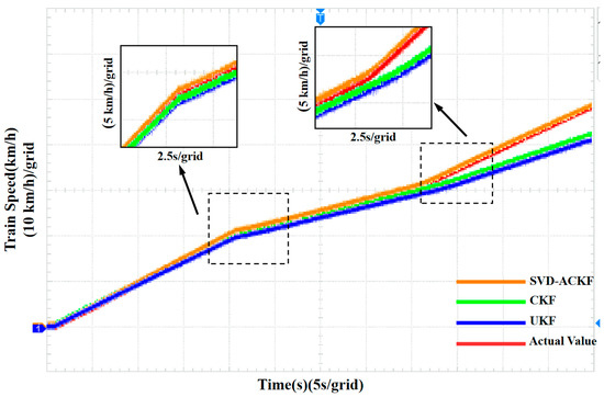
Figure 12. Comparison of SVD-ACKF, CKF, UKF and actual value for train speed.

At t = 0 s, the CKF speed curve exhibited a slightly faster startup characteristic, while the initial speed response of UKF lagged behind CKF. SVD-ACKF had a slower startup, but its speed curve surpassed CKF at t = 8 s and maintained closer alignment with the actual value thereafter. This indicates that during the initial identification phase, SVD-ACKF achieved superior transient stability and tracking precision compared to CKF and UKF.

At t = 20 s, the rail surface became wet, causing changes in adhesion characteristics that required the control system to make adaptive adjustments. As shown in the left enlarged figure of Figure 12 (time scale: 2.5 s/grid), calculations of the percentage deviation of speed between each control algorithm and the actual value at this time point revealed that the speed deviation of SVD-ACKF was 2.71%, which was 1.86% lower than CKF’s 4.39% and 4.25% lower than UKF’s 6.46%. This result confirmed that SVD-ACKF maintained better tracking precision under wet rail conditions.

After t = 40 s, the rail surface returned to a dry state. As shown in the right enlarged figure of Figure 12 (time scale: 2.5 s/grid), calculations of the percentage deviation of speed between each control algorithm and the actual value during this phase showed that the SVD-ACKF speed curve closely aligned with the actual value, with a speed deviation of 2.48%, which was closest to the actual speed; both CKF and UKF speed curves exhibited a 10.53% speed deviation at t = 45 s, and the deviation continued to increase thereafter, failing to track changes in the actual speed. This indicates that SVD-ACKF had stronger robustness against disturbances during the transition from wet to dry rail conditions.

In summary, across all rail condition stages, SVD-ACKF outperformed CKF and UKF in terms of speed tracking precision, transient stability, and robustness against disturbances.

5. Conclusions and Future Work

In this paper, the train state estimation algorithm and adhesion control are combined, and a method of adhesion control based on high-speed train state estimation is proposed. A complete closed-loop simulation model is constructed. Different experimental conditions are tested, and the results are analyzed.

An optimized adhesion control method, based on adhesion peak point search, is proposed. This method uses the extreme value search algorithm to search for the optimal creep velocity and uses the backstepping method to output the control torque. However, in the actual train operation process, the acquisition and accuracy of the input parameters are also crucial to the realization of the current adhesion control method. Therefore, the adhesion coefficient estimated by the ASTF algorithm and the vehicle speed estimated by the SVD-ACKF algorithm are input into the adhesion closed-loop control and verified based on the MT PXI hardware-in-the-loop simulation platform. At the same time, the different time of the simulated carriage passing through the rail surface is used to verify the effectiveness and real-time performance of the adhesion control method.

The results show that the adhesion control based on state estimation can effectively estimate the vehicle speed and adhesion coefficient in real time during the operation of high-speed trains and can realize the adhesion control requirements. It consistently operates near the adhesion peak point, maintaining a high adhesion utilization level.

Furthermore, the SVD-ACKF algorithm, as the core component, integrates SVD with adaptive noise covariance updates. Hardware-in-the-loop tests show that its single-step computation time is 3.2 ms, and the total latency when combined with the full traction control logic is ≤8 ms. This performance meets the computational requirements of mainstream train control units (TCUs), which are typically equipped with industrial-grade DSPs or ARM processors (≥1 GHz), thus avoiding the need for high-performance hardware upgrades and ensuring cost-effective deployment.

Future work will focus on further validating its real-world applicability. Planned steps include (1) conducting compatibility tests on physical train TCUs to verify its performance under embedded hardware constraints; (2) performing on-vehicle experiments to assess long-term stability under varying rail conditions and climatic environments. These efforts will lay a solid foundation for the practical deployment of state estimation-based adhesion control in high-speed railway systems.

References

- Fernandez-Bobadilla, H.A.; Martin, U. Modern Tendencies in Vehicle-Based Condition Monitoring of the Railway Track. IEEE Trans. Instrum. Meas. 2023, 72, 3507344. [Google Scholar] [CrossRef]
- Zani, N.; Mazzù, A.; Solazzi, L.; Petrogalli, C. Examining Wear Mechanisms in Railway Wheel Steels: Experimental Insights and Predictive Mapping. Lubricants 2024, 12, 93. [Google Scholar] [CrossRef]
- Millan, P.; Pagaimo, J.; Magalhães, H.; Ambrósio, J. Clearance joints and friction models for the modelling of friction damped railway freight vehicles. Multibody Syst. Dyn. 2022, 58, 21–45. [Google Scholar] [CrossRef]
- Rahaman, M.L.; Bernal, E.; Spiryagin, M.; Bosomworth, C.; Sneath, B.; Wu, Q.; Cole, C.; McSweeney, T. An investigation into the effect of slip rate on the traction coefficient behaviour with a laboratory replication of a locomotive wheel rolling/sliding along a railway track. Tribol. Int. 2023, 187, 108773. [Google Scholar] [CrossRef]
- Tao, Y.; Yau, S.S.-T. Outlier-Robust Iterative Extended Kalman Filtering. IEEE Signal Process. Lett. 2023, 30, 743–747. [Google Scholar] [CrossRef]
- Pichlik, P.; Zdenke, J. Locomotive Wheel Slip Control Method Based on an Unscented Kalman Filter. IEEE Trans. Veh. Technol. 2018, 67, 5730–5739. [Google Scholar] [CrossRef]
- Tian, Y.; Wen, T.; Fang, X.; Wang, J.; Li, K.; Cai, B.; Roberts, C. Cross-Term Correlations Considered Extended Kalman Filter for High-Speed Train State Estimation. IEEE Sens. J. 2025, 25, 21971–21987. [Google Scholar] [CrossRef]
- Yuhao, H. Estimation of Vehicle Status and Parameters Based on Nonlinear Kalman Filtering. In Proceedings of the 2022 6th International Conference on Robotics and Automation Sciences (ICRAS), Wuhan, China, 9–11 June 2022; pp. 200–205. [Google Scholar]
- Huang, Z.; Fan, X.; Chen, M.; Peng, J. Joint estimation method of sideslip angle and tyre–road adhesion coefficient using extended Kalman filter and unscented Kalman filter. Veh. Syst. Dyn. 2025, 1–24. [Google Scholar] [CrossRef]
- Sun, H.; Wang, H. Research on Electric Vehicle Differential System Based on Vehicle State Parameter Estimation. Vehicles 2025, 7, 80. [Google Scholar] [CrossRef]
- Bertipaglia, A.; Alirezaei, M.; Happee, R.; Shyrokau, B. An unscented kalman filter-informed neural network for vehicle sideslip angle estimation. IEEE Trans. Veh. Technol. 2024, 73, 12731–12746. [Google Scholar] [CrossRef]
- Pichlik, P.; Bauer, J. Adhesion characteristic slope estimation for wheel slip control purpose based on UKF. IEEE Trans. Veh. Technol. 2021, 70, 54303–54311. [Google Scholar] [CrossRef]
- Kobelski, A.; Osinenko, P.; Streif, S. Experimental verification of an online traction parameter identification method. Control. Eng. Pract. 2021, 113, 104837. [Google Scholar] [CrossRef]
- Ji, X.; Li, G.; Fan, D.S. Study on joint estimation of vehicle state and parameters. Comput. Simul. 2022, 39, 127–134. [Google Scholar]
- Hu, C.; Li, R.; Wong, P.K.; Dai, S.-L.; Xie, Z.; Zhao, J. ACKF-Based Finite-Time Prescribed Performance RISE Control for Asymptotic Trajectory Tracking of ASVs With Input Saturation. IEEE Trans. Veh. Technol. 2025, 74, 2715–2725. [Google Scholar] [CrossRef]
- Chang, R.; Chen, Z.; Yin, F. Distributed Kalman Filtering for Speech Dereverberation and Noise Reduction in Acoustic Sensor Networks. IEEE Sens. J. 2023, 23, 31027–31037. [Google Scholar] [CrossRef]
- Cortés, I.; van der Merwe, J.R.; Lohan, E.S.; Nurmi, J.; Felber, W. Performance evaluation of adaptive tracking techniques with direct-state Kalman filter. Sensors 2022, 22, 420. [Google Scholar] [CrossRef]
- Fossen, T.I. Line-of-sight path-following control utilizing an extended Kalman filter for estimation of speed and course over ground from GNSS positions. J. Mar. Sci. Technol. 2022, 27, 806–813. [Google Scholar] [CrossRef]
- Piaggio, B.; Garofano, V.; Donnarumma, S.; Alessandri, A.; Negenborn, R.; Martelli, M. Follow-the-Leader Guidance, Navigation, and Control of Surface Vessels: Design and Experiments. IEEE J. Ocean. Eng. 2023, 48, 997–1008. [Google Scholar] [CrossRef]
- Kangunde, V.; Mohutsiwa, L.O.; Jamisola, R.S. Feedback State Estimation for Multi-rotor Drones Stabilisation Using Low-Pass Filter and a Complementary Kalman Filter. In Proceedings of the 2021 International Conference on Unmanned Aircraft Systems (ICUAS), Athens, Greece, 15–18 June 2021; IEEE: New York, NY, USA, 2021. [Google Scholar]
- Ke, M. EKF-DT LocBump: Enhanced Real-Time 3D Localization and Terrain Bump Prediction with Sensor Fusion. In Proceedings of the 2024 4th International Conference on Electrical Engineering and Control Science (IC2ECS), Nanjing, China, 27–29 December 2024; pp. 480–487. [Google Scholar]
- Popa, G.; Andrei, M.; Tudor, E.; Vasile, I.; Ilie, G. Fast Detection of the Stick–Slip Phenomenon Associated with Wheel-to-Rail Sliding Using Acceleration Sensors: An Experimental Study. Technologies 2024, 12, 134. [Google Scholar] [CrossRef]
- Andrei, M.; Popa, G.; Ilie, G.; Tudor, E. Stick-Slip Movement in Driving Axles of Railway Vehicles equipped with Damping Devices. Electroteh. Electron. Autom. 2023, 71, 32–39. [Google Scholar] [CrossRef]
- He, J.; Zuo, X.; Zhang, C.; Mao, S.; He, Y. Anti-slip control based on optimal slip ratio for heavy-haul locomotives. J. Eng. 2019, 23, 9069–9074. [Google Scholar] [CrossRef]
- Wang, Y.; Wang, Z.; Shi, D.; Chu, F.; Guo, J.; Wang, J. Optimized Longitudinal and Lateral Control Strategy of Intelligent Vehicles Based on Adaptive Sliding Mode Control. World Electr. Veh. J. 2024, 15, 387. [Google Scholar] [CrossRef]
- Cheng, C.; Wang, W.; Meng, X.; Shao, H.; Chen, H. Sigma-mixed unscented Kalman filter-based fault detection for traction systems in high-speed trains. Chin. J. Electron. 2023, 32, 982–991. [Google Scholar] [CrossRef]
- Hu, H.; Bei, S.; Zhao, Q.; Han, X.; Zhou, D.; Zhou, X.; Li, B. Research on Trajectory Tracking of Sliding Mode Control Based on Adaptive Preview Time. Actuators 2022, 11, 34. [Google Scholar] [CrossRef]
- Fang, X.; Lin, S.; Yang, Z.; Lin, F.; Sun, H.; Hu, L. Adhesion Control Strategy Based on the Wheel-Rail Adhesion State Observation for High-Speed Trains. Electronics 2018, 7, 70. [Google Scholar] [CrossRef]
- Liu, J.; Peng, Q.; Huang, Z.; Liu, W.; Li, H. Enhanced sliding mode control and online estimation of optimal slip ratio for railway vehicle braking systems. Int. J. Precis. Eng. Manuf. 2018, 19, 655–664. [Google Scholar] [CrossRef]
- Ohyama, T. Some basic studies on the influence of surface contamination on adhesion force between wheel and rail at higher speeds. Railw. Tech. Res. Inst. Q. Rep. 1989, 30, 127–135. [Google Scholar]
- Kadowaki, S.; Ohishi, K.; Miyashita, I.; Yasukawa, S. Re-adhesion control of electric motor coach based on disturbance observer and sensor-less vector control. In Proceedings of the Power Conversion Conference-Osaka 2002 (Cat. No.02TH8579), Osaka, Japan, 2–5 April 2002. [Google Scholar]
- Ishikawa, Y.; Kawamura, A. Maximum adhesive force control in super high speed train. In Proceedings of the Power Conversion Conference-PCC’97, Nagaoka, Japan, 6 August 1997; IEEE: New York, NY, USA, 1997; Volume 2, pp. 951–954. [Google Scholar]
- Zhao, X.; Li, J.; Yan, X.; Ji, S. Robust Adaptive Cubature Kalman Filter and Its Application to Ultra-Tightly Coupled SINS/GPS Navigation System. Sensors 2018, 18, 2352. [Google Scholar] [CrossRef] [PubMed]
- Kulikova, M.V.; Kulikov, G.Y. SVD-based factored-form cubature Kalman filtering for continuous-time stochastic systems with discrete measurements. Automatica 2020, 120, 109110. [Google Scholar] [CrossRef]
- Zhang, Y.; Wang, J.; Sun, Q.; Gao, W. Adaptive cubature Kalman filter based on the variance-covariance components estimation. J. Glob. Position. Syst. 2017, 15, 1. [Google Scholar] [CrossRef]
Disclaimer/Publisher’s Note: The statements, opinions and data contained in all publications are solely those of the individual author(s) and contributor(s) and not of MDPI and/or the editor(s). MDPI and/or the editor(s) disclaim responsibility for any injury to people or property resulting from any ideas, methods, instructions or products referred to in the content. |
© 2025 by the authors. Licensee MDPI, Basel, Switzerland. This article is an open access article distributed under the terms and conditions of the Creative Commons Attribution (CC BY) license (https://creativecommons.org/licenses/by/4.0/).