Abstract
The scarcity of explicit feedback data is a major challenge in the design of recommender systems. Although such data are of a high quality due to users’ voluntary provision of numerical ratings, collecting a sufficient amount in real-world service environments is typically infeasible. As an alternative, implicit feedback data are extensively used. However, because implicit feedback represents observable user actions rather than direct preference statements, it inherently suffers from ambiguity as a signal of true user preference. To address this issue, this study reinterprets the ambiguity of implicit feedback signals as a problem of epistemic uncertainty regarding user preferences and proposes a latent factor model that incorporates this uncertainty within a Bayesian framework. Specifically, the behavioral vector of a user, which is learned from implicit feedback, is restructured within the embedding space using attention mechanisms applied to the user’s interaction history, forming an implicit preference representation. Similarly, item feature vectors are reinterpreted in the context of the target user’s history, resulting in personalized item representations. This study replaces the deterministic attention scores with stochastic attention weights treated as random variables whose distributions are modeled using a Bayesian approach. Through this design, the proposed model effectively captures the uncertainty stemming from implicit feedback within the vector representations of users and items. The experimental results demonstrate that the proposed model not only effectively mitigates the ambiguity of preference signals inherent in implicit feedback data but also achieves better performance improvements than baseline models, particularly on datasets characterized by high user–item interaction sparsity. The proposed model, when integrated with an attention module, generally outperformed other MLP-based models in terms of NDCG@10. Moreover, incorporating the Bayesian attention mechanism yielded an additional performance gain of up to 0.0531 compared to the model using a standard attention module.
1. Introduction
A recommender system is a type of personalized information filtering system that predicts and suggest items to users based on their previous interaction history. Therefore, user–item interaction history has become the most critical data component in the design and operation of recommender systems. The importance of these interaction data is particularly pronounced in collaborative filtering approaches, which rely solely on user and item identifiers and interaction records without incorporating any additional metadata. Interaction history refers to a user’s past feedback on items, which can take various forms such as views, cart additions, purchases, and ratings. Among these, rating data are considered relatively noise-free because they explicitly reflect the user’s preference and its intensity toward the observed item. However, in real-world service environments, collecting sufficient explicit feedback data for algorithmic training is typically difficult. Alternatively, implicit feedback data are increasingly being used to train recommendation models.
However, implicit feedback data, such as view, cart, and purchase histories, only indicate whether an action has occurred and do not directly reflect a user’s preference for an item. Thus, models that leverage implicit feedback must include an additional step to infer the presence and intensity of user preferences from the observed behavior. The most straightforward approach is to treat observed and unobserved interactions as preference and non-preference indications, respectively. However, this binary classification oversimplifies the underlying data by ignoring the fact that both observed and unobserved interactions occur under specific decision-making pathways and contextual constraints. This approach introduces systematic interpretational bias, because it disregards cases in which a user may have observed and subsequently disliked an item or have never been exposed to it. Consequently, observations and non-observations are forcibly categorized into binary preference classes without accounting for these important nuances [].
In collaborative filtering models that rely primarily on interaction history without auxiliary information, the systematic misinterpretation of implicit feedback data can introduce uncertainty in parameter estimation and preference prediction. This issue originates from the rigid classification of observed and unobserved interactions as binary indicators of preference and non-preference, respectively. To overcome this challenge, previous studies have proposed one-class collaborative filtering (OCCF) methods, which avoid making definitive assumptions about the user’s preference based solely on observed or unobserved interactions. For example, some approaches develop objective functions that optimize pairwise preference rankings between observed and unobserved item pairs for each user []. Others assign confidence weights proportional to the frequency of observed interactions [], or distinguish between exposure and interactions, modeling the exposure process explicitly to refine preference inference [].
This study reinterprets the limitations of using implicit feedback data by framing the core issue as the uncertainty in definitively equating user interactions to actual preferences. Although previous research has focused on structurally compensating for this epistemic uncertainty during the model training phase, such approaches typically fail to explicitly incorporate the uncertainty into the model architecture. To bridge this gap, we propose a latent factor model that directly captures the epistemic uncertainty associated with user preference signals through Bayesian attention-based representations of users and items, redefined within the user’s interaction history. Furthermore, the proposed model adopts a probabilistic ranking objective function, specifically leveraging the likelihood term from Bayesian personalized ranking (BPR) [], to optimize preference orderings in a stochastic framework.
In the field of recommender systems, various models have been proposed to incorporate uncertainty into the modeling process [,,,,,]. Among these, some have employed attention mechanisms or Bayesian inference techniques. However, the Bayesian attention-based model proposed in this study differs in its intended use from such prior approaches.
Attention-based models like DACR and NAIS exemplify the existing methods [,]. DACR applies a self-attention module at the input stage of the latent factor model to emphasize informative signals and suppress noise by attending over interaction vectors and their linear transformations. NAIS, on the other hand, uses an attention mechanism in item-based collaborative filtering to dynamically select and aggregate key history items depending on the target item. In contrast, our proposed model aims to recalibrate the behavioral representations derived from ID embeddings by conditioning them on the user’s history, thereby constructing a context-aware preference representation within a latent factor framework.
Similarly, Bayesian inference-based models such as BPMF and Mult-VAE have also been introduced [,]. BPMF treats the vector representations in a latent factor model as random variables to account for uncertainty in parameter estimation caused by data sparsity and to prevent overfitting. Mult-VAE incorporates stochasticity in the encoding and decoding process of the interaction vector, thereby addressing the uncertainty in interpreting implicit feedback as definitive signals of user preference. In contrast, our model seeks to represent the uncertainty inherent in trusting the alignment between the target user or item and their historical context as indicative of true user preference.
Thus, while existing models employing attention or Bayesian methods serve important roles, our Bayesian attention framework is uniquely designed to capture epistemic uncertainty arising from the ambiguous link between user behavior and preference within local history-based representations.
The remainder of this paper is organized as follows. Section 2 provides an overview of latent factor models, OCCF, and the Bayesian attention module (BAM). Section 3 introduces the proposed model in detail. Section 4 outlines the experimental setup designed to validate the performance improvements of the proposed model compared with existing approaches, and the corresponding results and interpretations are presented in Section 5. Finally, Section 6 concludes this study by summarizing the key findings and recommending future research directions.
2. Related Works
2.1. Latent Factor Model for Collaborative Filtering
Collaborative filtering methods are generally categorized into two primary approaches: memory- and model-based. The memory-based approach selects items to recommend by computing vector similarities directly from the user–item interaction matrix. Although this approach is simple and does not require the training of a separate predictive model, it typically achieves high performance. However, its major limitation is its inability to recommend items for which no prior user interaction data exist. In contrast, the model-based approach constructs predictive models that learn user preferences or likelihoods of interaction with items rather than relying solely on similarity measures. This approach addresses some limitations of memory-based methods by enabling recommendations for previously unseen or non-interacted items.
Among various model-based methods, the latent factor model is one of the most widely utilized. This method assumes that a set of underlying latent factors can be used to represent the interactions between users and items. Accordingly, both users and items are mapped to low-dimensional vectors comprising these latent features. Based on these representations, a predictive model is constructed to estimate user preferences, which are then used to generate item recommendations. The matrix factorization-based approach is a representative implementation of the latent factor model. In this approach, the user–item interaction matrix is decomposed into two lower-dimensional matrices, typically referred to as the user and item matrices, using matrix factorization techniques such as singular value decomposition []. The user and item matrices capture the latent feature vectors for users and items, respectively. With recent advances in deep learning, new variants of latent factor models have emerged, leveraging neural architectures to enhance representational capacity. These models can be broadly classified into two categories depending on how user and item vectors are derived: ID and history embeddings. The ID embedding approach uses one-hot vectors to encode users and items and learns their dense vector representations through embedding layers. In contrast, the history embedding approach constructs user and item vectors by embedding interaction histories derived from the user–item interaction matrix, such as the set of items a user has interacted with or the set of users who have interacted with a particular item.
A representative model using ID embedding is NeuMF []. In this model, user and item representations are learned through embedding layers applied to one-hot encoded IDs. NeuMF combines two modeling components: generalized matrix factorization, which extends conventional matrix factorization, and a multilayer perceptron (MLP). For each user and item, two separate embedding vectors are generated, one for each component, and these embeddings are used to predict whether a user–item interaction has occurred. In contrast, CFNet [] leverages history embedding. In CFNet, user embeddings are generated based on the vectors of items with which the user has interacted, whereas item embeddings are derived from the vectors of users who have interacted with the item. In other words, the model computes the respective embeddings using the row and column vectors of the user–item interaction matrix. Similar to NeuMF, CFNet employs two linear embedding layers to generate two distinct embeddings for both users and items. These embeddings are then used to compute a matching score that reflects the likelihood of interaction between a given user and item.
2.2. Implicit Feedback Data
As previously mentioned in Chapter 1, implicit feedback data refer to datasets that contain records of user interactions with items, such as views or purchases, without explicitly stated preferences or ratings. In this context, user behavior is indirectly inferred rather than explicitly expressed. Let M denote the total number of users and N denote the total number of items. The user–item interaction matrix for implicit feedback data can be represented as follows:
The definition of an interaction can vary depending on the analysis objective and the dataset. For example, an interaction may be defined as a user merely viewing an item or as a completed purchase. Importantly, the observation of an interaction between user u and an item i does not necessarily imply that the user favors the item. A user may view an item once but ultimately decide not to engage further after reviewing its details. Conversely, the absence of an observed interaction does not conclusively indicate disinterest. For example, a user may have failed to encounter a particular item, and the user may have shown a preference for it had it been discovered. In this respect, implicit feedback data inherently suffers from the ambiguity of user preference signals, which must be carefully addressed when designing recommendation models.
2.3. One-Class Collaborative Filtering
As previously noted, one of the main challenges in utilizing implicit feedback data is the difficulty in categorizing observed and unobserved interactions into binary preference labels. One-class collaborative filtering (OCCF) addresses this issue by treating unobserved interactions as uncertain or ambiguous signals rather than negative feedback []. In this framework, the interaction frequency, such as the number of views or purchases, is interpreted as an indication of the degree of confidence in a user’s preference rather than a direct measure of preference.
Various OCCF methodologies have been proposed, depending on how unobserved items are handled. Weighted regularized matrix factorization (WRMF), also referred to as implicit alternating least squares (iALS), is a well-known approach []. This model treats all user behaviors, such as clicks, views, or purchases, as positive feedback and performs matrix factorization by transforming the interaction logs into a binary preference matrix. However, recognizing that the absence of interaction does not necessarily imply disinterest, WRMF introduces confidence weights, assigning higher and lower weights to observed and unobserved interactions, respectively. This weighting scheme allows the model to account for data uncertainty while learning user–item representations. The model is trained using alternating least squares, which ensures efficient convergence even with large-scale datasets and has been extensively adopted in real-world recommender systems. Other studies have explored the probabilistic modeling of item exposure to distinguish between unobserved feedback due to disinterest and that due to lack of exposure. ExpoMF [], which explicitly incorporates item exposure into the modeling of implicit feedback, is a representative example. Unlike conventional methods, ExpoMF considers that a user’s decision not to interact with an item may stem from simply not having seen the item rather than having a negative preference. ExpoMF introduces a Bernoulli random variable to model the latent probability of item exposure and assumes that user selection is conditioned on exposure. This approach enables more cautious interpretation of unobserved feedback and mitigates issues such as popularity bias and unfairness in recommendations by separating exposure and preference in the modeling process.
The ranking optimization approach is another widely adopted methodology within the OCCF framework, with BPR being one of its most representative models []. Unlike conventional models that predict whether a user prefers a particular item, BPR focuses on learning the relative ordering of preferences. The model assumes that if user u has interacted with item i, user u is more likely to prefer item i to another item j with which no interaction has occurred. This is referred to as the pairwise ranking assumption. Let denote the preference space of user u and denote the set of model parameters used to predict rankings. Given observed user–item interaction data, the BPR framework aims to maximize the posterior probability of the model parameters . This is equivalent to finding the parameter set that maximizes , which is the product of the likelihood and the prior. is defined as the probability that a randomly selected user u prefers item i to item j. Furthermore, let us assume with . Then, the objective function for optimizing BPR can be formulated as follows:
Here, , where I denotes the set of all items and denotes the set of all items provided by the user.
If we decompose the predicted preference score as , then the probability that user u prefers item i over item j can be defined as . Consequently, the log-likelihood of the dataset D, given the model parameters , can be expressed as . This formulation implies that the BPR objective can be interpreted as the negative log-likelihood of the observed data. This property provides a theoretical basis for incorporating BPR as the log-likelihood term within the ELBO framework, as discussed later.
2.4. Bayesian Attention Module
The attention module is a mechanism designed to assist neural networks in focusing on specific parts of the input when computing output representations. This module primarily comprises three core components: query, key, and value. The query represents the target information or the basis for evaluating relevance to other vectors. The key serves as an index-like reference used to compare against the query, whereas the value contains the actual information to be retrieved, which is weighted according to its relevance to the query. Here, let Q, K, and V denote the matrices corresponding to the query, key, and value, respectively. In standard attention mechanisms, the attention weight matrix W is computed as follows:
The attention function can be defined in various ways, such as Luong attention [] or Bahdanau attention []. Subsequently, the result of this function is multiplied by the value matrix V, and the output is referred to as the attention score.
Most previous studies on attention mechanisms have assumed that attention weights are deterministic. However, such deterministic attention may be insufficient for modeling the complex dependencies inherent in the target data distribution. To address this limitation, some studies have proposed the use of stochastic attention. This approach treats attention weights as random variables and estimates their underlying distributions. The key characteristic of stochastic attention models is their probabilistic interpretation of attention, which allows for capturing uncertainty in the alignment between elements. Nevertheless, these methods typically face several challenges. In particular, gradient descent-based optimization becomes difficult, and in some cases, the attention weights do not satisfy the constraint of summing to one. Consequently, in practice, stochastic attention mechanisms typically exhibit inferior performance compared to their deterministic counterparts.
The BAM has been proposed to address the limitations associated with previous stochastic attention methods []. Similar to previous approaches, it treats attention weights as random variables and uses techniques such as variational inference to estimate their underlying distributions [,,]. However, a key distinction lies in the fact that the distributional estimation is performed within a Bayesian framework, which provides a principled way to model uncertainty and incorporate prior knowledge.
Here, assume that the attention weight W is a data-dependent local latent variable; let denote the prior distribution over W and denote the likelihood of the output . The distribution of W is then estimated through a variational distribution , which is parameterized by the output of the attention function applied to the query and key representations. The objective is to determine a distribution that minimizes , which quantifies the discrepancy between the variational and posterior distributions. By employing amortized variational inference, this objective can be equivalently reformulated as the maximization of the evidence lower bound (ELBO), providing a tractable optimization target.
Furthermore, the study emphasizes that the proposed Bayesian attention mechanism addresses the challenge of learning the distribution parameters in stochastic attention models. Specifically, it suggests employing reparametrizable distributions as the variational distribution for attention weights to improve effective optimization. The authors propose the use of distributions such as log-normal and Weibull distributions for this purpose. In addition, the study provides a detailed explanation of how these distributions can be reparametrized, enabling gradient-based learning through the reparameterization trick commonly used in variational inference. This approach allows for efficient backpropagation and improves the stability of training Bayesian attention models.
By employing the log-normal distribution in this study, the variational distribution can be optimized as follows. Let denote the random variable. The probability density function of this distribution is defined as
Here, and . If a sample S is drawn from a log-normal distribution , it can be reparameterized as follows:
Then, if is sampled and regarded as the unnormalized attention weight between the i-th query and the j-th key, the normalized attention weight can be computed by applying a normalization function , which normalizes the weights across all keys for each query. Consequently, the normalized attention weight becomes a reparameterizable function, allowing the backpropagation of gradients through the sampling process. This formulation enables the incorporation of stochasticity into the attention mechanism while preserving differentiability for efficient optimization.
Next, we describe how to compute the distribution parameters of the unnormalized attention weight S based on the query and key vectors. As previously discussed, the attention weights are assumed to follow a log-normal distribution. Here, denotes the result of applying an attention function to query Q and key K. The standard deviation term is treated as a global hyperparameter and the mean parameter is defined as . Sampling is equivalent, via the reparameterization trick, to sampling from the expression . This formulation allows the use of the attention score derived from applying an attention function to the query and key as a parameter in estimating the distribution of the unnormalized attention weights S. The attention scores obtained by applying an attention function to the query and key can be used to estimate the distribution of the unnormalized attention weights S. By subsequently applying a normalization function to S, the variational distribution of the normalized attention weights W can be constructed.
3. Proposed Method
As discussed in Section 2.2, implicit feedback data do not always accurately reflect a user’s true preferences. In other words, such data inherently contain ambiguity in user preference signals. Unlike the previous studies introduced in Section 2.3, this study assumes that observed user–item interactions contain uncertainty and proposes a Bayesian framework-based method that models this uncertainty. In particular, we propose the Bayesian attentional collaborative filtering (BACF) model, which integrates components of the BAM with elements from the NeuMF architecture [] to optimize personalized ranking. The overall structure of the proposed model is shown in Figure 1.
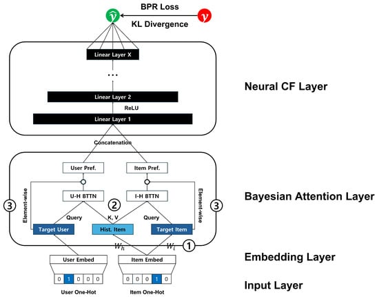
Figure 1.
The architecture of BACF model.
Here, let M and N denote the total numbers of users and items, respectively. When one-hot encoded user and item ID vectors are provided as inputs to the input layer, the corresponding user and item embedding vectors are obtained through an embedding layer, which is parameterized by the user embedding matrix and the item embedding matrix , where K represents the embedding dimension. To distinguish between the representations of an item when it serves as the target and history times for a target user, separate linear transformations are applied to the item embeddings. Let denote the linear transformation matrices used for the target and history item roles, respectively. When items are treated as target items, the transformed item matrix is computed as . Similarly, when items are considered history items, the transformed item matrix is given by . This design allows the proposed model to learn role-specific representations of items depending on their contextual usage within the user–item interaction framework.
The Bayesian attention layer reconstructs both the target user and item as a context vector derived from the target user’s interaction history. For a given user u, the user embedding vector is used as the query, and the embedding vectors of the user’s history items serve as the keys and values in the BAM. Here, the target item i is excluded from the history when constructing the attention input. This ensures that the context vector is learned solely from previously interacted items, thereby preventing information leakage during training. The resulting context vector represents the target user in the context of their past interactions and can be expressed as follows:
Similarly, the context vector of the target item, which is reconstructed based on its relationship to other items in the user’s history, can be obtained by applying the BAM. In this case, the embedding vector of the target item is used as the query, and the history item vectors are used as keys and values. This setup allows the proposed model to capture the relation between the target item and the user’s past interactions, thereby providing a context-aware representation of the item. The context vector for the target item can be formally expressed as follows:
These contextual vectors represent preference expressions conditioned on the target user’s interaction history. By performing element-wise multiplication with the previously obtained global behavioral representation, we extract latent preference signals.
Subsequently, the two latent signals are concatenated and passed through a multi-layer perceptron, followed by the application of a sigmoid activation function at the output layer to generate the final prediction.
In this formulation, the operation refers to the BAM, which includes layer normalization and a residual connection applied to the query vector. In addition, the vector combination-based similarity function proposed in NAIS was used as the attention weight function to compute the parameters of the variational distribution.
As the number of history items increases, attention weights may become overly flattened, resulting in uniformly low values. To address this issue, we introduce two normalization factors: the sharpening factor and the smoothing factor . The sharpening factor enhances the contrast between attention scores, thereby encouraging the model to focus more on highly relevant items by amplifying score differences. In contrast, the smoothing factor elevates the overall magnitude of the scores, ensuring that all items receive a non-negligible level of attention. Significant variations in the number of times in the histories of users can cause instability in learning the prior distribution, particularly when users with extensive interaction histories dominate the early stages of training. To address this issue, users are first segmented into n groups according to the size of their interaction histories. The training then proceeds sequentially, beginning with users with shorter histories. This incremental learning approach was adopted in NAIS [] to improve training stability by gradually introducing more complex user behavior patterns.
The training objective of the BACF model is to maximize the ELBO within the framework of variational inference. To enable ranking-based optimization, the BPR criterion is incorporated into the expected likelihood term of the ELBO. This integration allows the model to be trained with a direct focus on improving personalized ranking performance.
Here, u, i, and j represent the user, positive item, and negative item, respectively, where the positive item refers to an item with which the user has interacted, and the negative item refers to an item with which no interaction has been observed. Because the Bayesian attention mechanism is applied separately to the target user, positive item, and negative item, the corresponding Kullback–Leibler (KL) divergence terms are computed individually for each component. These KL terms are then aggregated to form the overall regularization term in the objective function.
4. Experiment
The proposed BACF model represents users and items as vectors while explicitly addressing the ambiguity of user preference signals by incorporating a stochastic component, namely the Bayesian attention module. To assess whether modeling such ambiguity leads to improved performance, we compare BACF against baseline methods that utilize implicit feedback without stochastic modules. Specifically, we selected several representative MLP-based latent factor models: NeuMF [] as a model based on ID embeddings; CFNet [] and DNCF [] as models utilizing history-based embeddings; and DACR [], which incorporates an attention module, along with its associated submodules. Furthermore, in the training of the Bayesian attention module within BACF, both the prior distribution and the variational distribution are modeled using the log-normal distribution.
4.1. Dataset
In this study, we used four publicly available datasets. Their characteristics are summarized in Table 1.

Table 1.
Data statistics.
The MovieLens dataset [] contains user rating data collected from the MovieLens movie recommendation platform. We use the MovieLens-Latest Small dataset, which includes approximately 100,000 user–item interactions. This dataset comprises explicit feedback data in the form of 1–5-star ratings. These ratings are converted into implicit feedback signals to align with the objectives of this study. Irrespective of the rating value, any recorded feedback is treated as an indication of an interaction and is mapped to a value of 1. Conversely, the absence of feedback is treated as no interaction and is mapped to 0. The Last.FM dataset [,] comprises user listening records collected from the Last.FM music streaming platform. Among its variants, this study uses the Last.FM-2K dataset, which was curated and released by the GroupLens research group at the University of Minnesota. It contains listening histories for 2,000 users, where the number of times a user has played songs by a specific artist is recorded. In this study, any recorded playback is treated as an interaction and converted to a value of 1, whereas the absence of playback is converted to a value of 0. The A-Beauty [,] and A-Music [,] datasets are derived from Amazon review data, specifically in the luxury-beauty and digital-music categories, and were collected and processed by Julian McAuley’s research team at the University of California, San Diego. This study uses the 5-core versions of these datasets, which include only users and items with at least five interactions. The datasets contain explicit feedback in the form of 1–5-star ratings. Consistent with our approach to implicit feedback modeling, any recorded rating is interpreted as an interaction and converted to a value of 1.
If we had used the original data, that is, the explicit feedback, as they were, it would have provided a more accurate reflection of users’ preferences. However, converting explicit feedback into implicit feedback may introduce user preference signal ambiguity. The degree of ambiguity varies with the characteristics of each dataset. For example, in the MovieLens dataset, approximately 13.4% of the feedback has ratings of 2 stars or below, which can reasonably be interpreted as negative preferences. When the original ratings are converted into binary implicit feedback, such cases are treated in the same way as 5-star ratings, both of which are considered positive interactions. This transformation introduces semantic ambiguity, because the system cannot distinguish between clear preferences and possible dislikes.
Taking this into account, the following characteristics are observed across the datasets. As shown in Table 1, the MovieLens dataset has lower data sparsity than the other datasets. However, it exhibits a high degree of ambiguity after conversion due to a relatively high proportion of low ratings. Similarly, the A-Beauty and A-Music datasets not only exhibit high sparsity but also contain low ratings below 2 stars, at 7.5% and 9.0%, respectively. Thus, similar to the MovieLens dataset, they have a high degree of ambiguity when converted to implicit feedback. In contrast, the Last.FM dataset exhibits substantially different characteristics. As previously explained, this dataset contains feedback in the form of play counts rather than explicit ratings. It can be reasonably assumed that lower and higher play counts indicate lower and higher preferences, respectively. Notably, only 0.69% of the user–artist interactions involve only one listen, and the proportion remains as low as 3.7%, even when expanded to include 10 or fewer listens. Thus, most interactions recorded as “1” in the implicit feedback data likely reflect genuine user interest, indicating that the degree of ambiguity in this dataset is relatively low.
4.2. Experiment Settings
For model training and evaluation, each dataset was split into training, validation, and test sets using stratified sampling based on users. The split ratio was fixed at 8:1:1. For negative sampling, a negative-to-positive sample ratio of 1:1 was applied for the training and validation sets, with negatives drawn randomly at each epoch. A ratio of 1:99 was applied for the test set.
For the MovieLens dataset, which contains up to approximately 2000 historical interactions per user, we limited the number of history items per user to 400 (top 10%) for computational efficiency. Items were selected based on term frequency-inverse document frequency scoring to prioritize more informative interactions.
To monitor early stopping, we constructed a leave-one-out evaluation set by selecting one positive sample per user that was excluded from the training, validation, and test sets. The negative samples in this set followed the same 1:100 sampling ratio used in the test set. The evaluation metrics were computed every 10 epochs rather than every epoch. The normalized discounted cumulative gain at rank 10 (NDCG@10) was used as the primary evaluation metric. Training was terminated early if NDCG@10 did not improve for 10 consecutive evaluations. A performance gain was recognized only if the improvement exceeded the threshold of 0.001. The final model evaluation was performed using the model parameters corresponding to the best observed performance rather than those from the final epoch. The final evaluation metrics included NDCG@5, NDCG@10, HitRatio@5, and HitRatio@10. To identify the optimal hyperparameter settings for both the proposed and baseline models, we conducted a grid search. The final set of selected hyperparameter configurations is presented in Table 2.
Table 2.
Experimental settings.
5. Results
5.1. Performance Comparison Across Deterministic Models
Table 3 compares the performance of the proposed and baseline models across the four datasets. The best-performing results in the following tables are indicated in bold. The proposed model consistently outperforms all baselines across all evaluation metrics, including the primary metric NDCG@10. Notably, the performance improvements of the proposed model are most significant on the A-Beauty and A-Music datasets, which suffer from high data sparsity and a high degree of ambiguity in user preference signals. On the MovieLens dataset, which exhibits low data sparsity but high preference ambiguity, the BACF model exhibits superior performance on all metrics, except HR@10, for which it ranks second. This result indicates that the BACF model is effective even in settings with rich user–item interaction histories. In contrast, on the Last.FM dataset, which features high sparsity but low ambiguity, a condition favorable to deterministic models, the DeepCF-ml module achieves higher HR@k scores. However, BACF still outperforms it in terms of NDCG@k scores, highlighting the strength of the proposed model in capturing ranking quality more effectively. These findings suggest that the proposed BACF model remains robust and performs competitively even in environments with minimal implicit feedback ambiguity in which deterministic approaches generally exhibit greater effectiveness.
Table 3.
Performance comparison (with BPR loss).
When compared based on NDCG@10, models utilizing history embeddings—such as DeepCF, DNCF, and DACR—demonstrated superior performance over NCF-based models that rely on ID embeddings. This trend was especially evident in datasets with lower interaction density, including Last.FM, A-Beauty, and A-Music. Although the proposed model is based on ID embeddings, it incorporates an attention mechanism to aggregate user history when generating the final vector representation. Accordingly, the performance gains of the proposed model stem from refining global behavioral representations using conditionally derived preference representations. However, the performance gap between the deterministic and Bayesian attention mechanisms was relatively smaller in Last.FM and A-Beauty, while it was more pronounced in MovieLens and A-Music. These variations in performance improvement suggest two key implications: (1) the lower the reliability of individual observations, the more beneficial Bayesian inference becomes; (2) even when individual observations are unreliable, if the average amount of user history, i.e., reference information, is insufficient, the benefits of Bayesian attention may be less apparent.
Meanwhile, although the proposed model, BACF, was trained using the BPR loss function, the baseline models were originally designed to be optimized with the Binary Cross-Entropy (BCE) loss function. In other words, for the baseline models in Table 3, using BCE is essential to achieving their best performance, and thus, the comparison under the BPR loss may not be entirely fair. To account for this, we additionally trained all baseline models using the BCE loss function, while BACF was trained with the BPR loss function, and evaluated their performance accordingly. The results are presented in Table 4. Even under this setting, where the baseline models are optimized using their original loss function, BACF still outperforms them, confirming the robustness and effectiveness of the proposed model.
Table 4.
Performance comparison (with BCE loss).
5.2. Effect of Bayesian Attention Module
In this study, we assumed that implicit feedback data inherently contains uncertainty and incorporated this uncertainty into the modeling process. To achieve this, we replaced the conventional attention mechanism with a Bayesian attention module, which treats attention weights not as fixed values but as probabilistic variables. To evaluate the effectiveness of this approach, we compared the proposed model—Bayesian Attentional Collaborative Filtering (BACF)—with two alternatives: the DACR model, which uses a standard attention mechanism, and an Attentive-CF variant of BACF that replaces the Bayesian attention module with a deterministic attention mechanism. The experimental results presented in Table 5 demonstrate that the proposed BACF model outperformed both DACR and Attentive-CF. This indicates that explicitly modeling the uncertainty in implicit feedback through a Bayesian attention framework leads to improved recommendation performance compared to using deterministic attention alone.
Table 5.
Comparison between attentive model and BACF model.
5.3. Importance of Prior Information Based on Data Sparsity and Preference Ambiguity
As described in Section 2.4, this study employs the log-normal distribution in the BAM design. In this setup, the standard deviation of the log-normal distribution functions as a global hyperparameter that must be manually specified by the user. This section investigates the effects of variations in this global hyperparameter on the performance of the BACF model.
Table 6 summarizes the experimental results, where the standard deviations of the prior and variational distributions are adjusted. The standard deviation of the variational distribution was varied across the values of 0.01, 0.1, 0.2, and 0.3, whereas the prior distribution was tested with standard deviations of 1.0 and 10.0. A prior with a standard deviation of 10.0 corresponds to a weakly informative prior, implying that it imposes minimal influence based on key-based prior knowledge. In contrast, a prior with a standard deviation of 1.0 represents a strongly informative prior that incorporates key-based prior information during inference.
Table 6.
Importance of prior information: setting standard deviation in log-normal distribution based on dataset characteristics.
The experimental results reveal that the performance of the BACF model is better when the standard deviation of the prior distribution is 1.0 than when it is 10.0. This finding shows that strong prior knowledge can serve as a valuable component in estimating the posterior distribution. The performance gap between the weak and strong prior information is particularly pronounced on the A-Beauty and A-Music datasets compared with the MovieLens and Last.FM datasets. This observation implies that the importance of prior knowledge increases with data sparsity.
Interestingly, despite also exhibiting high sparsity, the Last.FM dataset shows a smaller performance difference between the two priors. This may be because the Last.FM dataset exhibits low user preference signal ambiguity. In other words, even with sparse data, the observed data provide sufficient information for posterior estimation if each interaction delivers clear and consistent feedback about user preferences. Consequently, the impact of prior knowledge is reduced, which explains the smaller performance variation in the Last.FM experiments than in the experiments with more ambiguous datasets such as A-Beauty and A-Music.
5.4. Configuring Variational Distribution Based on Interaction Sparsity and Ambiguity
Table 7 summarizes the changes in the performance of the proposed model with respect to different standard deviation settings in the variational distribution under the condition that the standard deviation of the prior distribution is fixed at 1.0, reflecting a strong informative prior. The standard deviation of the variational distribution controls the degree to which uncertainty in the posterior distribution reflects both prior knowledge and the observed data.
Table 7.
Setting standard deviation of log-normal distribution used for variational distribution.
In the MovieLens dataset, which exhibits the highest interaction density but low reliability per interaction (i.e., high ambiguity), the best performance is achieved when the standard deviation is set to a relatively low value. This result suggests that data richness and redundancy allow for a precise posterior belief to be formed even when individual observations contain ambiguous signals. In contrast, the Last.FM dataset, characterized by high reliability per observation (low ambiguity) but extremely sparse interaction data, resulted in optimal performance with a larger standard deviation in the variational distribution. This implies that the limited number of observations provides only a partial view of users’ complex preferences despite the clarity of each preference signal, which increases uncertainty in the posterior distribution.
Based on these findings, the following guideline can be established for configuring the standard deviation of the variational distribution. Data sparsity is the primary driver of posterior estimation epistemic uncertainty. Therefore, in low-sparsity settings, even when data are ambiguous, setting the standard deviation lower is appropriate, allowing for more confident posterior inferences. Conversely, in high-sparsity settings, even if ambiguity is relatively low, it is advisable to increase the standard deviation to better reflect the uncertainty arising from the limited quantity of observed data.
5.5. Complexity Analysis
This study was conducted using an Nvidia GeForce RTX 4060 Ti GPU. Figure 2 illustrates the time required per epoch and the number of epochs until convergence for three models across each dataset: the MLP module of NCF, Attentive-CF (which replaces the Bayesian attention module in BACF with a standard attention module), and the proposed BACF model. While the BACF model consistently outperforms the others in terms of recommendation accuracy, it requires substantially longer training time. This indicates a need for further optimization to improve the model’s training efficiency.
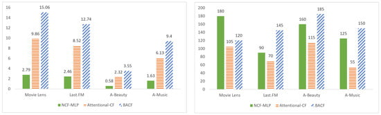
Figure 2.
Comparison of training time. (Left): Time required per epoch (seconds/epoch). (Right): Number of epochs until training convergence.
6. Conclusions
This study addresses the challenges associated with implicit feedback data by redefining the ambiguity of user preference signals as a problem of epistemic uncertainty regarding user preferences. In this regard, a model specifically designed to operate under such cognitive limitation conditions is proposed. Compared with previous research, the proposed model makes the following contributions.
First, the proposed model explicitly distinguishes between behavior and preference matching. The former is modeled through user and item embedding vectors, whereas the latter is represented via contextual embeddings derived from users’ histories of interacted items. Second, the proposed model directly incorporates the uncertainty in preference matching caused by behavior-matching data. This is achieved by introducing stochasticity into the attention scores between target users and their historical items within the attention mechanism, thereby capturing probabilistic variations. Third, the identity of the target item, expressed in the embedding space, is reinterpreted within the context of the target user’s past experiences. Although user history does not explicitly reflect preferences, the proposed model adjusts the embedding of the target item based on the behavioral context, enabling the derivation of a personalized semantic representation from the user’s perspective.
The experimental results demonstrate that the proposed model consistently outperformed the existing deterministic models across all four datasets. The performance improvement was more pronounced in environments with greater underlying ambiguity in the data and a lower interaction density. These results suggest that the Bayesian framework is effective in settings with epistemic uncertainty. Given that the attention mechanism exclusively references user history, the model shows potential for enhanced performance in environments where new items are frequently introduced. However, when comparing the A-Beauty and A-Music datasets, greater performance improvement was observed in A-Music, where, despite similar sparsity levels, users had a relatively richer interaction history. These findings suggest that the proposed model is more effective in sparse data environments when a sufficient amount of user history is available. Furthermore, the proposed model appropriately balanced the influence of prior knowledge and observational data by tuning the scale parameters of both the variational and prior distributions. This enabled the model to adjust the reliability of posterior beliefs based on interaction sparsity and data quality, thereby ensuring stable performance under various data conditions.
However, the proposed model still presents several areas for improvement. Firstly, while the current study evaluated the model using four datasets, further validation on a broader range of datasets is necessary to more robustly demonstrate its effectiveness. Additionally, in the MovieLens dataset—which has the lowest level of data sparsity—the maximum number of user history items was limited to the top 10% (400 items) per user due to computational inefficiency. This highlights the need to improve the efficiency of posterior distribution estimation in the Bayesian attention module, particularly when dealing with large-scale interaction data and low sparsity environments. Moreover, the overall training time of the model remains relatively high and should be further optimized in future work. Finally, the model’s performance is sensitive to how the prior distribution is configured, indicating a potential limitation in its robustness and stability across different settings.
Author Contributions
Conceptualization, J.W. and J.L.; methodology, J.W.; software, J.W.; validation, J.W. and J.L.; formal analysis, J.W. and J.L.; investigation, J.W. and J.L.; resources, J.W.; data curation, J.W.; writing—original draft preparation, J.W.; writing—review and editing, J.W. and J.L.; visualization, J.W. and J.L.; supervision, J.W. and J.L. All authors have read and agreed to the published version of the manuscript.
Funding
This research received no external funding.
Data Availability Statement
All data used in this study are publicly available. How the data can be accessed is described in the text, and a download link is provided in the reference.
Conflicts of Interest
The authors declare no conflicts of interest.
References
- Lerche, L. Using Implicit Feedback for Recommender Systems: Characteristics, Applications, and Challenges. Ph.D. Thesis, TU Dortmund University, Dortmund, Germany, 2016. [Google Scholar]
- Rendle, S.; Freudenthaler, C.; Gantner, Z.; Schmidt-Thieme, L. BPR: Bayesian Personalized Ranking from Implicit Feedback. In Proceedings of the Twenty-Fifth Conference on Uncertainty in Artificial Intelligence (UAI’09), Montreal, QC, Canada, 18–21 June 2009; pp. 452–461. [Google Scholar]
- Hu, Y.; Koren, Y.; Volinsky, C. Collaborative Filtering for Implicit Feedback Datasets. In Proceedings of the 2008 Eighth IEEE International Conference on Data Mining (ICDM 2008), Pisa, Italy, 15–19 December 2008; pp. 263–272. [Google Scholar]
- Liang, D.; Charlin, L.; McInerney, J.; Blei, D.M. Modeling User Exposure in Recommendation. In Proceedings of the 25th International Conference on World Wide Web (WWW 2016), Montreal, QC, Canada, 11–15 April 2016; pp. 951–961. [Google Scholar]
- He, X.; He, Z.; Song, J.; Liu, Z.; Jiang, Y.-G.; Chua, T.-S. NAIS: Neural Attentive Item Similarity Model for Recommendation. IEEE Trans. Knowl. Data Eng. 2018, 30, 2354–2366. [Google Scholar] [CrossRef]
- Cui, C.; Qin, J.; Ren, Q. Deep collaborative recommendation algorithm based on attention mechanism. Appl. Sci. 2022, 12, 10594. [Google Scholar] [CrossRef]
- Salakhutdinov, R.; Mnih, A. Bayesian probabilistic matrix factorization using Markov chain Monte Carlo. In Proceedings of the 25th International Conference on Machine Learning, Hensinki, Finland, 5–9 July 2008; pp. 880–887. [Google Scholar]
- Liang, D.; Krishnan, R.G.; Hoffman, M.D.; Jebara, T. Variational autoencoders for collaborative filtering. In Proceedings of the 2018 World Wide Web Conference, Lyon, France, 23–27 April 2018; pp. 689–698. [Google Scholar]
- Forouzandeh, S.; Berahmand, K.; Rostami, M.; Aminzadeh, A.; Oussalah, M. UIFRS-HAN: User interests-aware food recommender system based on the heterogeneous attention network. Eng. Appl. Artif. Intell. 2024, 135, 108766. [Google Scholar] [CrossRef]
- Forouzandeh, S.; DW, P.M.; Jalili, M. DistillHGNN: A Knowledge Distillation Approach for High-Speed Hypergraph Neural Networks. In Proceedings of the 13th International Conference on Learning Representations, Singapore, 24–28 April 2025. [Google Scholar]
- Ahmadian, S.; Berahmand, K.; Rostami, M.; Forouzandeh, S.; Moradi, P.; Jalili, M. Recommender Systems based on Non-negative Matrix Factorization: A Survey. IEEE Trans. Artif. Intell. 2025, 1, 1–21. [Google Scholar] [CrossRef]
- He, X.; Liao, L.; Zhang, H.; Nie, L.; Hu, X.; Chua, T.S. Neural Collaborative Filtering. In Proceedings of the 26th International Conference on World Wide Web (WWW ’17), Perth, Australia, 3–7 April 2017; pp. 173–182. [Google Scholar]
- Deng, Z.-H.; Huang, L.; Wang, C.-D.; Lai, J.-H.; Yu, P.S. DeepCF: A Unified Framework of Representation Learning and Matching Function Learning in Recommender System. In Proceedings of the AAAI Conference on Artificial Intelligence (AAAI-19), Honolulu, HI, USA, 27 January–1 February 2019; pp. 61–68. [Google Scholar]
- Luong, M.-T.; Pham, H.; Manning, C.D. Effective Approaches to Attention-based Neural Machine Translation. In Proceedings of the 2015 Conference on Empirical Methods in Natural Language Processing (EMNLP 2015), Lisbon, Portugal, 17–21 September 2015. [Google Scholar]
- Bahdanau, D.; Cho, K.; Bengio, Y. Neural Machine Translation by Jointly Learning to Align and Translate. In Proceedings of the 3rd International Conference on Learning Representations (ICLR 2015), San Diego, CA, USA, 7–9 May 2015. [Google Scholar]
- Fan, X.; Zhang, S.; Chen, B.; Zhou, M. Bayesian Attention Modules. In Proceedings of the Advances in Neural Information Processing Systems 33 (NeurIPS 2020), Vancouver, BC, Canada, 6–12 December 2020; pp. 16362–16376. [Google Scholar]
- Deng, Y.; Kim, Y.; Chiu, J.; Guo, D.; Rush, A.M. Latent Alignment and Variational Attention. In Proceedings of the 32nd Conference on Neural Information Processing Systems (NeurIPS 2018), Montreal, QC, Canada, 2–8 December 2018; pp. 9735–9747. [Google Scholar]
- Shankar, S.; Sarawagi, S. Posterior Attention Models for Sequence to Sequence Learning. In Proceedings of the International Conference on Learning Representations (ICLR 2019), New Orleans, LA, USA, 6–9 May 2019. [Google Scholar]
- Lawson, D.; Chiu, C.-C.; Tucker, G.; Raffel, C.; Swersky, K.; Jaitly, N. Learning Hard Alignments with Variational Inference. In Proceedings of the 2018 IEEE International Conference on Acoustics, Speech and Signal Processing (ICASSP), Calgary, AB, Canada, 15–20 April 2018; pp. 5799–5803. [Google Scholar]
- He, G.; Zhao, D.; Ding, L. Dual-embedding based Neural Collaborative Filtering for Recommender Systems. arXiv 2021, arXiv:2102.02549. [Google Scholar] [CrossRef]
- Harper, F.M.; Konstan, J.A. The MovieLens Datasets: History and Context. ACM Trans. Interact. Intell. Syst. 2015, 5, 1–19. [Google Scholar] [CrossRef]
- Last.fm Website. Available online: http://www.lastfm.com (accessed on 1 March 2025).
- HatRec 2011|GroupLens Website. Available online: https://grouplens.org/datasets/hetrec-2011/ (accessed on 1 March 2025).
- Ni, J.; Li, J.; McAuley, J. Justifying Recommendations using Distantly-Labeled Reviews and Fine-Grained Aspects. In Proceedings of the 2019 Conference on Empirical Methods in Natural Language Processing and the 9th International Joint Conference on Natural Language Processing (EMNLP-IJCNLP), Hong Kong, China, 3–7 November 2019. [Google Scholar]
- Amazon Review Data. Available online: https://cseweb.ucsd.edu/~jmcauley/datasets/amazon_v2/ (accessed on 23 March 2025).
- He, R.; McAuley, J. Ups and Downs: Modeling the Visual Evolution of Fashion Trends with One-Class Collaborative Filtering. In Proceedings of the 25th International World Wide Web Conference (WWW 2016), Montreal, QC, Canada, 11–15 April 2016; pp. 507–517. [Google Scholar]
- Amazon Product Data. Available online: https://cseweb.ucsd.edu/~jmcauley/datasets/amazon/links.html (accessed on 23 March 2025).
Disclaimer/Publisher’s Note: The statements, opinions and data contained in all publications are solely those of the individual author(s) and contributor(s) and not of MDPI and/or the editor(s). MDPI and/or the editor(s) disclaim responsibility for any injury to people or property resulting from any ideas, methods, instructions or products referred to in the content. |
© 2025 by the authors. Licensee MDPI, Basel, Switzerland. This article is an open access article distributed under the terms and conditions of the Creative Commons Attribution (CC BY) license (https://creativecommons.org/licenses/by/4.0/).