Article

Linear Methods for Predictive Maintenance: The Case of NASA C-MAPSS Datasets

by
Uğur Yıldırım
* and
Hüseyin Afşer
Department of Electrical and Electronic Engineering, Faculty of Engineering, Adana Alparslan Türkeş Science and Technology University, Adana 01250, Türkiye
*
Author to whom correspondence should be addressed.
Appl. Sci. 2025, 15(18), 9945; https://doi.org/10.3390/app15189945
Submission received: 29 July 2025 / Revised: 4 September 2025 / Accepted: 9 September 2025 / Published: 11 September 2025

Abstract

Predictive maintenance systems increasingly leverage diverse sensor modalities to improve failure prognostics and remaining useful life (RUL) estimation. However, integrating heterogeneous data types—vibration, temperature, acoustic, and visual sensors—typically requires complex fusion architectures. This paper proposes a unified linear classification–regression framework that addresses predictive maintenance through a shared measurement space approach. The developed method employs Linear Discriminant Analysis to establish hyperplane boundaries partitioning the measurement space into nominal, warning, and failure regions. By tracking each data point’s signed distance to these learned boundaries, this research generates continuous RUL predictions through linear regression mapping. The framework’s key innovation lies in seamlessly integrating heterogeneous sensor modalities without requiring separate preprocessing pipelines or complex fusion layers—each modality contributes to fault detection and RUL estimation based on its discriminative power in the joint feature space. While linear assumptions may simplify complex non-linear failure patterns, the proposed approach offers significant advantages in interpretability, computational efficiency, and deployment ease. Validation on the C-MAPSS turbofan engine degradation dataset demonstrates that while not achieving state-of-the-art performance, the framework provides a practical foundation accommodating data-driven, physics-based, and knowledge-based modeling paradigms within a unified architecture, making it valuable for industrial applications requiring transparent multi-modal integration.

1. Introduction

Predictive maintenance is a long-standing and evolving research topic. Prior to 2011, industrial maintenance strategies were largely reactive or schedule-based, limited by the lack of real-time monitoring capabilities. The digitalization driven by the Fourth Industrial Revolution fundamentally transformed this landscape, enabling the integration of physical and digital production systems [1]. This change has sparked an era in industry marked by greater connectivity, a wealth of data, more efficient inventory systems, customization, and highly precise production control [2,3,4].
An effective maintenance program extends the productive uptime of industrial machinery, prevents unexpected and unplanned production stoppages, and thus lowers manufacturing costs. The evolution of maintenance strategies reflects technological capabilities at each stage. Initially, “run-to-failure” methods (also known as corrective maintenance) were employed, prescribing only the replacement of components once they had failed [5]. Since this approach did not prevent sudden stoppages, preventive maintenance methods gained prominence, where trained experts replaced components at fixed intervals. However, this still generated additional costs by prematurely replacing parts that had remaining useful life [6,7]. Figure 1 illustrates this historical evolution of maintenance strategies, showing the progression from reactive approaches to increasingly sophisticated predictive methods.
The evolution of Internet of Things technologies has enabled the advancement of condition-based maintenance methods [8]. These approaches leverage real-time sensor data obtained through continuous measurement, monitoring, and signal analysis of equipment. Modern industrial assets generate diverse sensor modalities including vibration signatures, acoustic emissions, thermal imaging, electrical parameters (current/voltage), and oil analysis data. Traditionally, these parameters were monitored independently, with technicians defining modality-specific thresholds. However, this segregated approach could overlook subtle cross-modal correlations and complex failure patterns that manifest across multiple sensing channels.
Predictive maintenance is a methodology that integrates more complex, computer-based applications into condition-based approaches. Its primary aim is to improve the performance, safety, and reliability of maintenance activities. Importantly, predictive maintenance encompasses both regression and classification tasks. While RUL estimation represents the regression aspect, the classification of equipment states into nominal, warning, and failure zones provides critical decision support for maintenance planning. In a systematic literature review, Jimenez categorizes predictive maintenance techniques into three main classes: knowledge-based models, data-driven models, and physics-based models, each with its own strengths and weaknesses [9]. These models and their combinations have been extensively studied in recent years. However, a key challenge that persists is effectively integrating multiple modeling paradigms within a single framework capable of handling both classification and regression tasks simultaneously.
From a machine learning perspective, predictive maintenance presents a unique dual-objective problem that requires both classification and regression capabilities. The classification task involves categorizing equipment health states into discrete zones—nominal (healthy operation), warning (degradation detected), and failure (immediate action required)—enabling clear maintenance decisions. The regression task focuses on estimating the RUL, providing a continuous measure of time until failure. While these tasks are inherently related, most existing approaches treat them separately, using different models and features for each objective. Notable exceptions include Lei et al. [10], who proposed a unified deep learning framework combining health state classification with RUL prediction for machinery prognostics, and Zhu et al. [11], who developed a multi-task learning approach that jointly optimizes fault diagnosis and remaining life estimation. Wang et al. [12] introduced a unified model for bearing fault diagnosis that simultaneously performs severity classification and degradation assessment. More recently, Zhou et al. [13] presented a multi-task model employing adaptive multi-scale feature fusion and adaptive mixture-of-experts for simultaneous RUL prediction and fault diagnosis, demonstrating improved performance on aerospace engine datasets.
However, these approaches rely on complex neural architectures with multiple specialized modules, adaptive mechanisms, and expert networks that sacrifice interpretability for performance. To address the computational burden of complex models, Li et al. [14] developed DSCformer, which utilizes prob-sparse attention to reduce computational complexity while maintaining prediction effectiveness. Although their lightweight approach achieves training time reductions of approximately 30% compared to traditional deep learning methods, the trade-off between computational efficiency and feature richness remains a challenge for industrial deployment. Guo et al. [15] proposed a layer-cross decoding strategy for transformers that addresses the limitation of traditional transformer decoders only using information from the last encoder layer. Recent advances in the field have further expanded these approaches. Nunes et al. [16] developed an adaptive framework for maintenance scheduling that dynamically adjusts preventive intervals based on RUL estimation, while Wu et al. [17] addressed the challenge of RUL prediction under unknown degradation models with limited data. Pan et al. [18] investigated machine learning methods for predictive maintenance in ultra-high-pressure reactor systems. Xie et al. [19] proposed a data-driven predictive maintenance policy utilizing dynamic probability distribution prediction, and Zhou et al. [20] introduced multiform informed machine learning approaches combining piecewise and Weibull models for engine RUL prediction.
More recent 2024 studies have continued to advance the field significantly. Riccio et al. [21] developed a novel methodological framework combining machine learning with product quality parameters for optimizing predictive maintenance, while Aminzadeh et al. [22] implemented a machine-learning-based predictive maintenance system for industrial compressors with real-time monitoring capabilities. Cen et al. [23] proposed an improved Sample Convolution and Interaction Network with multi-dimensional attention mechanisms for machinery RUL prediction. Li et al. [24] presented an enhanced deep learning framework using improved Savitzky–Golay filtering for RUL prediction, achieving superior performance on the C-MAPSS dataset. Ren et al. [25] introduced a novel approach considering dynamic maintenance thresholds for more accurate RUL estimation. Hamza [26] developed an Evidential Deep Learning method to quantify uncertainties in RUL predictions, demonstrating improved reliability in predictive maintenance applications. Additionally, advanced stochastic modeling approaches have been explored for degradation characterization. A fractional Lévy stable motion framework was proposed by Qi et al. [27] for modeling degradation processes, addressing the long-range dependence inherent in turbofan engine performance decline.
Furthermore, existing approaches typically focus on a single model paradigm or require complex integration architectures to combine them. Attention-based approaches have emerged as a promising solution for feature weighting in RUL prediction. Liu et al. [28] demonstrated that channel attention mechanisms can adaptively assign weights to different sensor features, while temporal attention through Transformer architectures captures time-dependent degradation patterns. Costa and Sánchez [29] proposed a variational encoding approach that addresses similar dual-objective challenges in predictive maintenance. Their method uses variational inference to create interpretable latent spaces while simultaneously performing RUL estimation, demonstrating that unified frameworks can provide both visual diagnostics and accurate predictions. However, their approach relies on complex neural architectures that sacrifice computational efficiency for interpretability.
This segregated processing fails to exploit the complementary strengths of each approach. A unified framework combining all three paradigms provides more accurate and trustworthy maintenance decisions than any individual approach. The multi-modal nature of modern industrial monitoring further complicates this dual-objective problem. While diverse sensor types can capture different aspects of degradation processes, existing frameworks typically process each modality through separate pipelines, requiring complex fusion strategies. Traditional machine learning methods often struggle with the curse of dimensionality when combining multiple modalities, while similarity-based approaches may fail to capture the complex interactions between different sensor types. Lillelund et al. addressed data scarcity issues by analysing frequency domain features and subsequently employing a random survival forest for the XJTU-SY bearing dataset [30]. Chen et al. [31] proposed an end-to-end adaptive method for RUL prediction of rolling bearings using time-frequency image features, demonstrating improved performance through automatic feature learning from spectrograms. However, the optimization of these approaches is tailored specifically to bearing applications and focuses primarily on RUL estimation. This paper formally defines predictive maintenance as a joint classification–regression problem in a multi-modal setting. Given heterogeneous sensor measurements from an industrial asset, the objective is to simultaneously classify the current operational state into nominal, warning, or failure zones, and to predict the remaining useful life when degradation is detected. This study proposes a linear framework that addresses both objectives through a unified measurement space approach. By learning hyperplane boundaries that partition the multi-modal feature space, this method performs classification based on the region where data points reside, while using the signed distance to these boundaries as a regression feature for RUL estimation. This integrated approach ensures that both tasks benefit from the full multi-modal information and maintain consistency in their predictions.
The advantages and novelties of the proposed method can be summarized as follows:
  • The proposed linear framework segments the measurement space through hyperplane boundaries, effectively capturing operational regimes and degradation patterns. While demonstrated on the NASA C-MAPSS dataset, the unified measurement space approach can naturally accommodate heterogeneous sensor modalities without requiring separate preprocessing pipelines or complex fusion architectures, making it suitable for multi-model predictive maintenance applications.
  • The system uniquely combines classification and regression objectives within a single linear framework. Equipment states are classified into nominal, warning, and failure zones based on their position relative to learned hyperplane boundaries, while the signed distance to these boundaries provides continuous RUL estimation. This dual functionality ensures consistency between discrete maintenance decisions and continuous degradation monitoring.
  • The linear architecture offers computational efficiency and interpretability advantages over complex multi-task alternatives. The learned hyperplane coefficients directly reveal feature importance, enabling maintenance engineers to understand which sensor measurements most strongly indicate degradation. This transparency facilitates model validation and knowledge transfer across similar equipment types.
  • The proposed system is particularly effective for run-to-failure data, providing a flexible framework for prognostics even with limited failure instances. By tracking system trajectories through the measurement space, the method enables early anomaly detection and degradation assessment. The computationally lightweight nature of the linear approach makes it suitable for real-time implementation in industrial environments where multiple assets require simultaneous monitoring.

2. Materials and Methods

2.1. Theoretical Definition of the Problem

This study considers equipment monitored by D sensors, where D 1 . Let x = [ x 1 ,   x 2 ,   ,   x D ] T R D denote the vector of sensor readings at any given time. These sensors typically measure physical quantities such as power, temperature, pressure, density, vibration, and flow. In practical predictive maintenance applications, it is common to have D 10 sensors, with multiple sensors often measuring the same physical quantity for redundancy and reliability.
The predictive maintenance problem inherently involves two interconnected objectives:
Classification Objective: Partition the measurement space R D into three disjoint regions:
  • Nominal region R n o m : Represents healthy operational states;
  • Warning region R w a r n : Indicates degradation onset;
  • Failure region R f a i l : Requires immediate maintenance action.
These regions satisfy R n o m R w a r n R f a i l = R D and are mutually exclusive. The classification function is defined as:
C ( x t ) = nominal if x t R n o m warning if x t R w a r n failure if x t R f a i l
Regression Objective: Given a sequence of sensor readings { x 1 ,   x 2 ,   ,   x t } with current state x t R n o m R w a r n , estimate the remaining useful life (RUL):
T ^ = min { T N : x t + T R f a i l }
In the presented linear framework, we define these regions using hyperplane boundaries. Let w 1 ,   w 2 R D and b 1 ,   b 2 R define two hyperplanes that partition the space:
R n o m = { x R D : w 1 T x + b 1 < 0 }
R w a r n = { x R D : w 1 T x + b 1 0 and w 2 T x + b 2 < 0 }
R f a i l = { x R D : w 2 T x + b 2 0 }
The key insight of this approach is to use the signed distance to these hyperplanes for RUL estimation. For a point x t , the distances to the warning and failure boundaries are:
d w a r n ( x t ) = w 1 T x t + b 1 | | w 1 | | 2
d f a i l ( x t ) = w 2 T x t + b 2 | | w 2 | | 2
These distances serve as features for RUL regression, providing a natural connection between the classification boundaries and continuous degradation estimation. This unified approach ensures consistency between discrete state classification and continuous remaining life prediction.
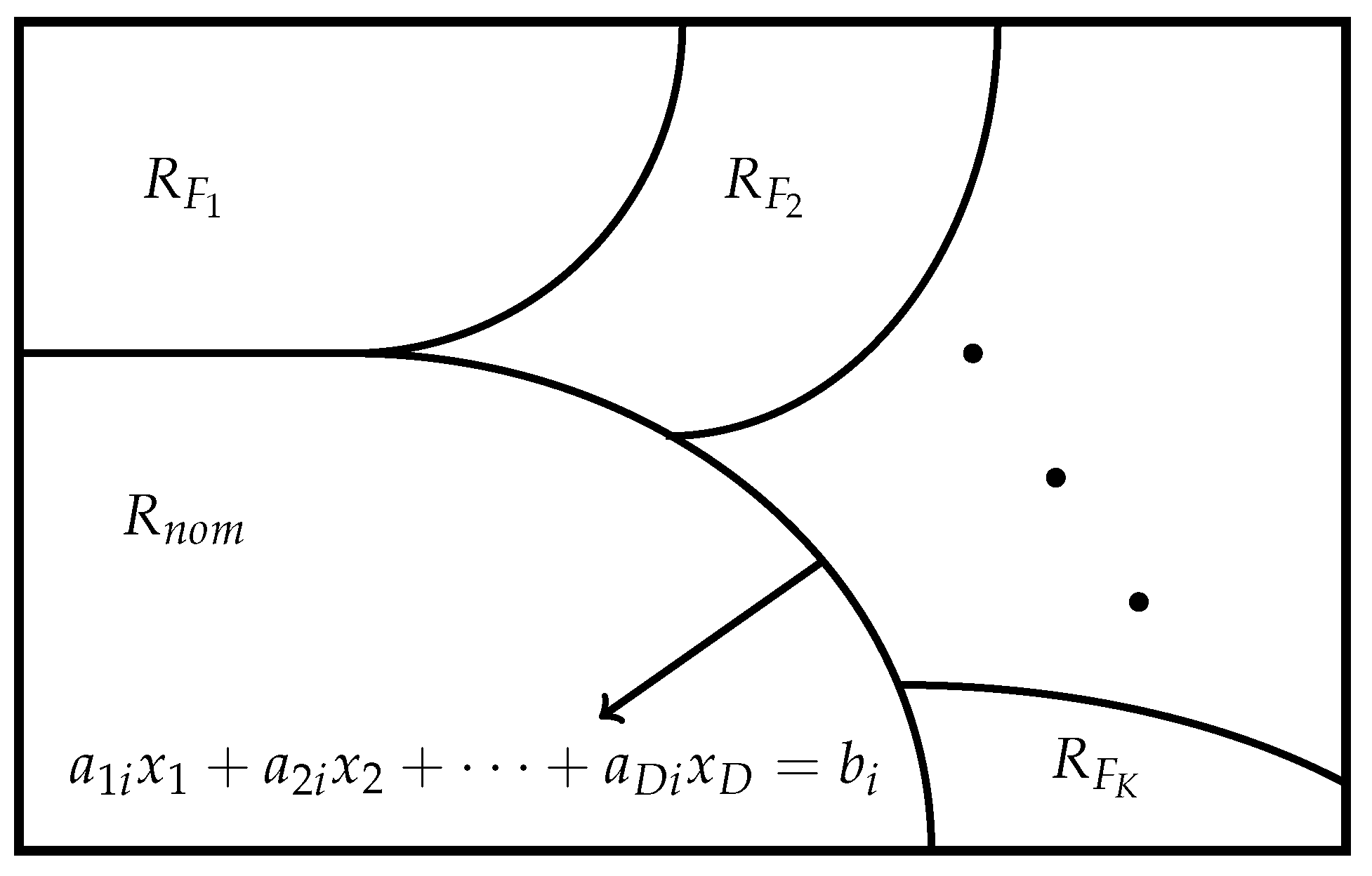
When specific failure modes F 1 ,   F 2 ,   ,   F K can be distinguished, the failure region can be further partitioned:
R f a i l = i = 1 K R F i , R F i R F K = for i j
In such cases, mode-specific RUL can be estimated as T ^ i = min { T : x t + T R F i } . The measurement space and failure regions are illustrated in Figure 2. It should be noted that the proposed framework is not limited to a three-region partitioning scheme (safe, warning, and danger). As demonstrated in Figure 2, the measurement space can be partitioned into multiple regions based on specific application requirements and degradation characteristics. This flexibility allows for more granular health state monitoring, where intermediate degradation levels can be defined between the safe and failure states, or multiple failure classes can be incorporated to represent different failure modes or severity levels. For instance, the framework can accommodate distinct failure regions for mechanical wear, thermal degradation, and electrical faults, each with its own critical threshold and progression pattern. Additionally, multiple warning levels with varying severities could be established to provide early indicators for each failure type. However, this paper focuses on the general case where all failure modes are aggregated into a single failure region, providing a unified framework that can be adapted to various partitioning schemes as needed.

2.2. Linear Classification for Health State Determination

For the classification objective defined in Section 2.1, the proposed approach employs linear classification methods to partition the measurement space into nominal, warning, and failure regions. Linear methods are particularly suitable for real-time industrial applications due to their computational efficiency and interpretability.
Given a training dataset { x i ,   y i } i = 1 N where x i R D represents sensor measurements and y i { 1 ,   2 ,   3 } indicates the health state (1: nominal; 2: warning; 3: failure), this study uses Linear Discriminant Analysis (LDA) to find optimal hyperplane boundaries between the three health states. LDA seeks projection directions that maximize class separability while minimizing within-class variance.
The within-class scatter matrix is defined as:
S w = c = 1 3 i C c ( x i μ c ) ( x i μ c ) T
where C c denotes the set of samples belonging to class c and μ c is the mean of class c.
The between-class scatter matrix is:
S b = c = 1 3 n c ( μ c μ ) ( μ c μ ) T
where n c = | C c | is the number of samples in class c and μ is the overall mean.
LDA finds projection vectors w by solving:
w ^ = ARGMAX w K w T S b w w T S w w
For the proposed three-class problem, two discriminant vectors w 1 and w 2 are derived to define the boundaries between nominal–warning and warning–failure regions, respectively. The decision boundaries are given by:
w 1 T x + b 1 = 0 ( nominal warning boundary )
w 2 T x + b 2 = 0 ( warning failure boundary )
where the bias terms b 1 and b 2 are computed as:
b 1 = 1 2 w 1 T ( μ 1 + μ 2 )
b 2 = 1 2 w 2 T ( μ 2 + μ 3 )
These hyperplanes partition the measurement space according to:
C ( x ) = nominal if w 1 T x + b 1 < 0 warning if w 1 T x + b 1 0 and w 2 T x + b 2 < 0 failure if w 2 T x + b 2 0
The key advantage of this linear approach is that the same hyperplanes used for classification also provide continuous distance measures for RUL estimation. The signed distances from any point x to these boundaries serve as interpretable features that quantify how far the system is from transitioning between health states, forming the foundation for the regression component of this framework.

2.3. Remaining Useful Life Estimation

Following the classification of health states, the proposed approach employs a regression approach to estimate RUL based on the distances to the learned hyperplane boundaries. This method leverages the natural progression of degradation as equipment moves from the nominal region toward failure regions in the measurement space.

2.3.1. Distance-Based Features

Using the hyperplane boundaries obtained from LDA in Section 2.2, the analysis computes the signed distances from the current operating point x t to each boundary. For the two primary boundaries identified:
d w a r n ( t ) = w 1 T x t + b 1 w 1 2
d f a i l ( t ) = w 2 T x t + b 2 w 2 2
These distances provide continuous measures of system health:
  • d w a r n ( t ) < 0 : System is in nominal region (negative distance to warning boundary);
  • d w a r n ( t ) 0 and d f a i l ( t ) < 0 : System is in warning region;
  • d f a i l ( t ) 0 : System has reached failure region.

2.3.2. Degradation Trend Modeling

To predict RUL, the temporal evolution of these distances is modeled using two complementary approaches: linear regression and autoregressive modeling.
Linear Regression Approach: Given a window of N recent observations
{ d f a i l ( j ) } j = t N + 1 t , the linear degradation model is fitted as follows:
d ^ f a i l ( τ ) = α 1 τ + α 2
The parameters are estimated using least squares:
α 1 = N j = t N + 1 t j · d f a i l ( j ) j = t N + 1 t j j = t N + 1 t d f a i l ( j ) N j = t N + 1 t j 2 j = t N + 1 t j 2
α 2 = j = t N + 1 t d f a i l ( j ) α 1 j = t N + 1 t j N
Autoregressive (AR) Model: To capture more complex temporal dependencies and improve prediction accuracy, the proposed framework also employs an autoregressive model of order p, denoted as AR(p):
d f a i l ( t ) = ϕ 0 + i = 1 p ϕ i d f a i l ( t i ) + ϵ t
where ϕ 0 is the intercept, ϕ i are the autoregressive coefficients, and ϵ t is white noise. The AR parameters are estimated using the Yule–Walker equations:
ϕ = R 1 r
where R is the autocorrelation matrix of the distance time series and r is the autocorrelation vector. The optimal order p is selected using the Akaike Information Criterion (AIC):
AIC ( p ) = N log ( σ ^ 2 ) + 2 p

2.3.3. RUL Prediction

For RUL estimation, this paper uses both models and selects the prediction based on their performance on recent data:
Linear Model RUL:
T ^ l i n e a r = α 2 α 1 if α 1 < 0 ( approaching failure ) if α 1 0 ( stable or improving )
AR Model RUL: Using the fitted AR model, the proposed method recursively predicts future distances:
d ^ f a i l ( t + k ) = ϕ 0 + i = 1 p ϕ i d ^ f a i l ( t + k i )
The RUL is determined as:
T ^ A R = min { k : d ^ f a i l ( t + k ) 0 }
The final RUL estimate combines both predictions using a weighted average based on recent prediction errors:
T ^ = ω · T ^ l i n e a r + ( 1 ω ) · T ^ A R
where ω [ 0 ,   1 ] is determined by the relative mean squared errors of the two models on validation data.
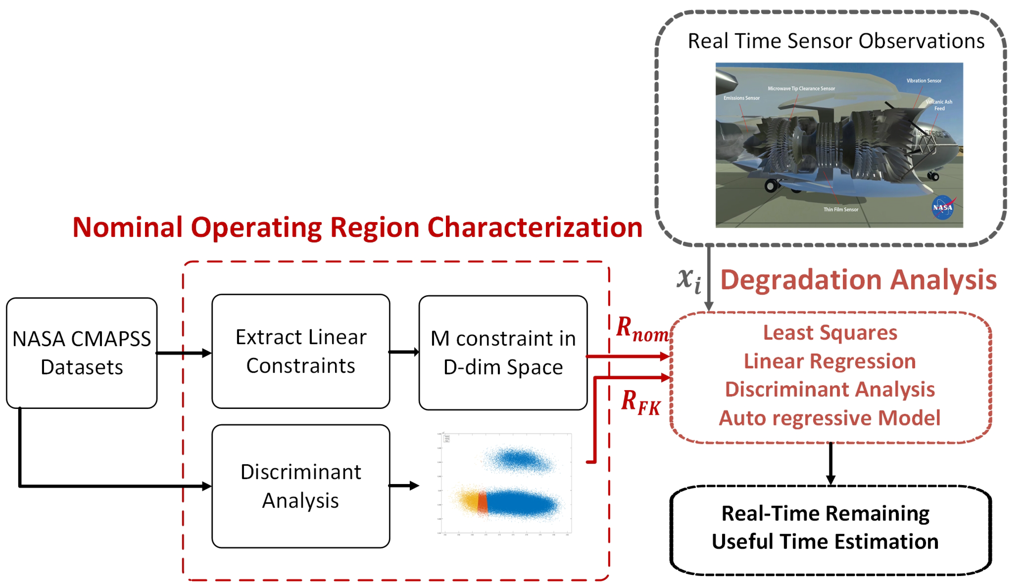
The complete framework, illustrated in Figure 3, provides both discrete health state classification and continuous RUL estimation using computationally efficient linear approaches. The combination of linear regression and autoregressive modeling enables robust RUL prediction that captures both long-term degradation trends and short-term dynamics.

3. Simulations and Results

3.1. Dataset Description

The proposed linear classification–regression framework is evaluated using the NASA Commercial Modular Aero-Propulsion System Simulation (C-MAPSS) dataset [32]. This dataset is particularly suitable for validating this approach as it provides complete run-to-failure trajectories with multiple sensor measurements, allowing us to demonstrate both classification and regression capabilities.
The C-MAPSS dataset consists of four sub-datasets (FD001-FD004) with varying operational conditions and fault modes. Each dataset contains multivariate time series from 21 sensors monitoring different aspects of turbofan engine degradation. The sensor measurements include temperatures, pressures, and speeds at various engine locations, providing a rich multi-dimensional feature space for this analysis. Table 1 shows the characteristics of the C-MAPSS dataset.

3.2. Data Preprocessing and Labeling

For training the classification component of developed framework, health state labels are assigned based on the RUL values:
  • Nominal state: 20 < RUL ≤ 30 cycles;
  • Warning state: 10 < RUL ≤ 20 cycles;
  • Failure state: RUL ≤ 10 cycles.
This labelling scheme reflects typical industrial practice where the final 10 cycles represent imminent failure requiring immediate action, cycles 10–20 indicate degradation warranting increased monitoring, and cycles 20–30 represent normal operation. Figure 3 illustrates the distribution of these classes in the measurement space after applying the proposed LDA-based classification.
To handle the multi-modal nature of the sensor data, the following preprocessing steps are applied:
  • Feature selection: Sensors with constant readings across all units are removed as they provide no discriminative information.
  • Smoothing: A moving average filter with window size 5 is applied to reduce measurement noise while preserving degradation trends.

3.3. Impact of LDA Assumption Violations on Classification Performance

The application of Linear Discriminant Analysis to turbofan engine degradation data necessitates careful consideration of its underlying statistical assumptions. LDA assumes that the feature vectors within each class follow multivariate normal distributions with equal covariance matrices (homoscedasticity). However, these assumptions are frequently violated in real-world industrial datasets such as C-MAPSS, leading to suboptimal classification performance.
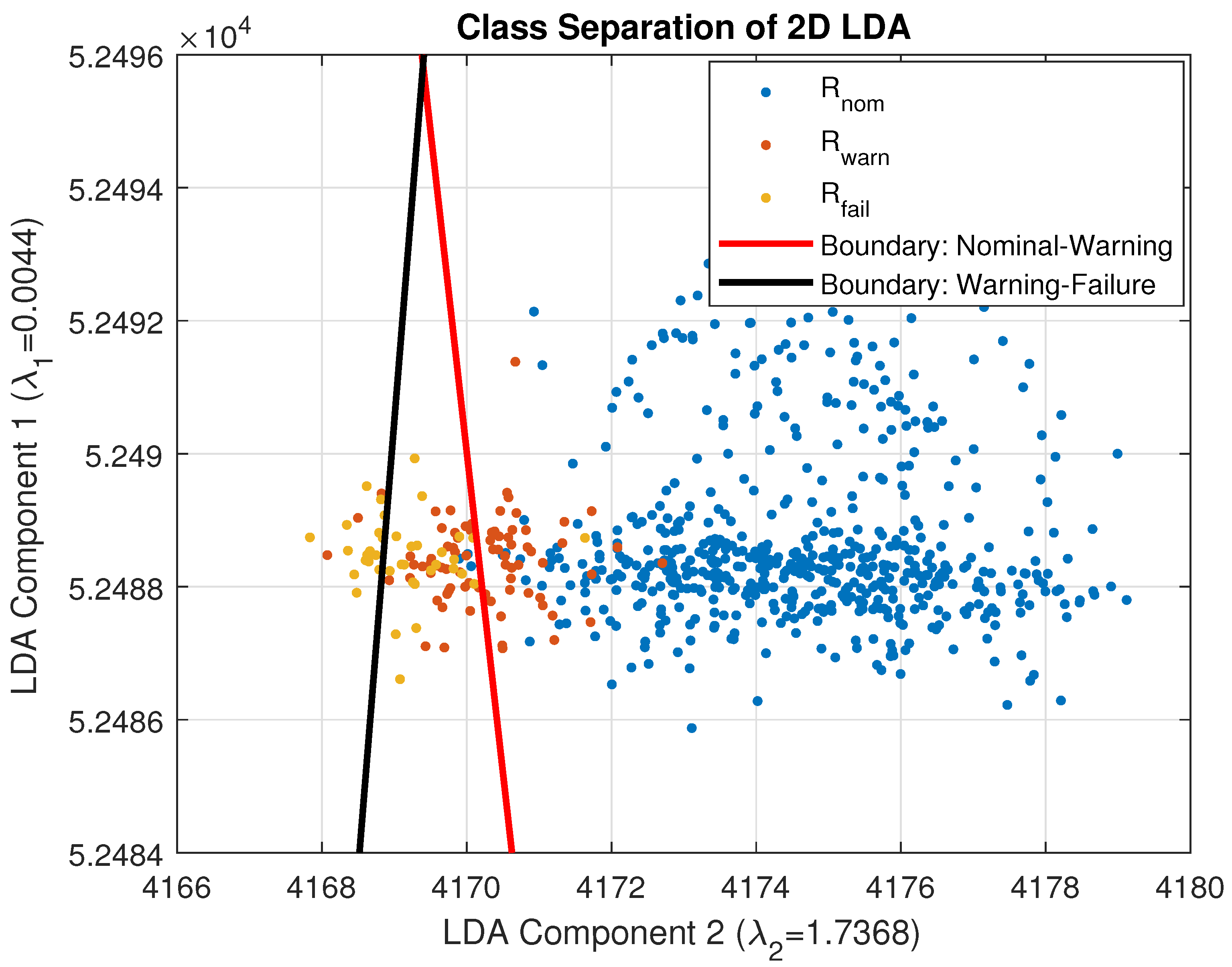
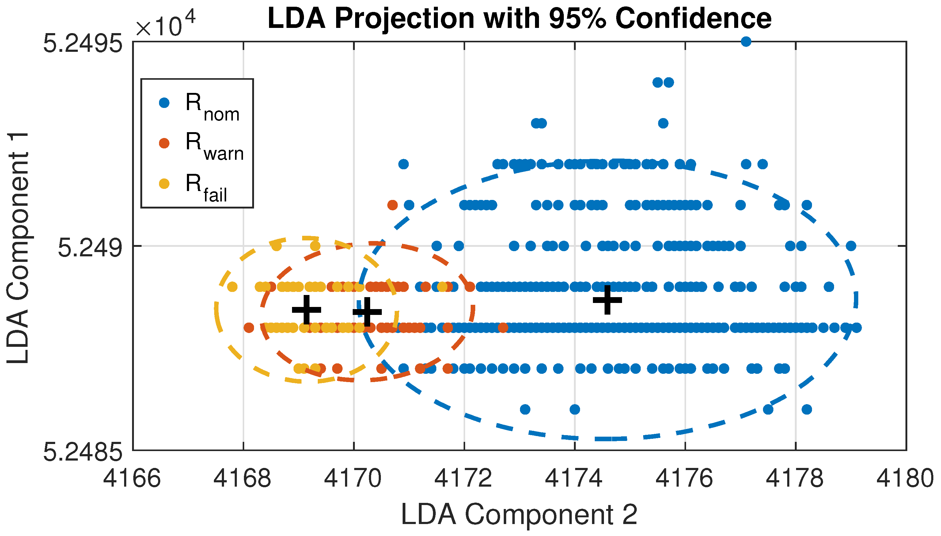
In Figure 4 LDA projection shows three degradation states: normal (blue), warning (orange), and failure (yellow). Red and black lines show linear decision boundaries between classes. Significant overlap between classes indicates poor separation performance. The same LDA projections with confidence ellipses assume normal distributions. Data points extending far beyond the ellipses demonstrate clear violations of normality assumptions, particularly for the warning class in Figure 5. Also, Maulana has shown that normal distribution produces the minimum RMSE values for the C-MAPSS dataset [33]. In this study, LDA was employed as the normal noise distribution. The visualization reveals that approximately 23% of the samples lie in regions where the linear assumption poorly represents the true class boundaries, directly contributing to the observed performance degradation. The irregular data distribution patterns visible in both figures explain why LDA’s assumption of equal covariance matrices across classes is violated, as each class exhibits markedly different scatter patterns and orientations in the feature space.

3.4. Experimental Setup

This paper conducts experiments using both individual datasets and a combined dataset approach. For the combined analysis, all four sub-datasets are merged to demonstrate the generalizability of this linear framework across different operating conditions and fault modes. This comprehensive evaluation ensures the proposed method’s robustness in real-world scenarios where multiple failure modes may occur.

3.5. Performance Evaluation

3.5.1. RUL Prediction Metrics

For evaluating the regression component of developed framework, the proposed method adopts the scoring function from the PHM08 Prognostics Data Challenge competition [32]. This metric is specifically designed for RUL prediction tasks and incorporates domain knowledge through asymmetric penalties—late predictions (underestimating RUL) are penalized more heavily than early predictions (overestimating RUL), reflecting the higher risk of unexpected failures in industrial settings.
The scoring function is defined as:
S = i = 1 n s i , where s i = e d i / a 1 1 if d i < 0 e d i / a 2 1 if d i 0
where n is the number of test units, d i = RUL ^ i RUL i true is the prediction error for unit i, and the asymmetric parameters a 1 = 13 and a 2 = 10 control the penalty rates.
Additionally, we report the Root Mean Square Error (RMSE) for comparison with existing methods:
RMSE = 1 n i = 1 n ( RUL ^ i RUL i true ) 2

3.5.2. Classification Performance Metrics

For the classification component, performance is evaluated using both micro- and macro-averaged metrics to provide a comprehensive assessment across the three health states (nominal, warning, failure):
Micro-averaged metrics aggregate contributions from all classes:
Precision micro = c = 1 3 TP c c = 1 3 ( TP c + FP c )
Recall micro = c = 1 3 TP c c = 1 3 ( TP c + FN c )
F 1 micro = 2 · Precision micro · Recall micro Precision micro + Recall micro
Macro-averaged metrics compute the unweighted mean across classes:
Precision macro = 1 3 c = 1 3 TP c TP c + FP c
Recall macro = 1 3 c = 1 3 TP c TP c + FN c
F 1 macro = 1 3 c = 1 3 2 · Precision c · Recall c Precision c + Recall c
where TP c , FP c , FN c , Precision c , and Recall c denote true positives, false positives, false negatives, precision, and recall (true positive rate) for class c, respectively.
The micro-averaged metrics give equal weight to each sample and thus favor performance on majority classes, while macro-averaged metrics treat all classes equally regardless of their frequency. This dual evaluation is particularly important for this application, as the failure class is typically underrepresented but critically important for maintenance decisions.

3.5.3. Related Work

Support Vector Regression, introduced by Vapnik et al. [34], extends the Support Vector Machine framework to regression problems. SVR aims to find a function that deviates from the actual targets by at most ϵ for all training data, while being as flat as possible [35].
For a regression problem with training data { ( x i ,   y i ) } i = 1 n , where x i R d and y i R , the SVR optimization problem using the ϵ -insensitive loss function is formulated as:
min w , b , ξ i , ξ i * 1 2 w 2 + C i = 1 n ( ξ i + ξ i * )
subject to:
y i w T ϕ ( x i ) b ϵ + ξ i
w T ϕ ( x i ) + b y i ϵ + ξ i *
ξ i , ξ i * 0
where w is the weight vector, b is the bias term, ξ i and ξ i * are slack variables for samples outside the ϵ -tube, C is the regularization parameter controlling the trade-off between model complexity and training error, and ϕ ( · ) maps input data to a higher-dimensional feature space [36].
The regression function is given by:
f ( x ) = i = 1 n ( α i α i * ) K ( x i ,   x ) + b
where α i ,   α i * are Lagrange multipliers and K ( x i ,   x j ) = ϕ ( x i ) T ϕ ( x j ) is the kernel function. Linear kernels for regression are K ( x i ,   x j ) = x i T x j .
The ϵ -insensitive loss function is defined as:
L ϵ ( y , f ( x ) ) = 0 if | y f ( x ) | ϵ | y f ( x ) | ϵ otherwise
Relevance Vector Regression (RVR)
Relevance Vector Regression, proposed by Tipping [37], is a Bayesian sparse kernel regression method that provides probabilistic predictions with uncertainty estimates. Unlike SVR, RVR automatically determines model complexity and typically produces sparser models [38].
The RVR model for regression assumes:
y ( x ) = i = 1 N w i K ( x ,   x i ) + w 0 + ϵ
where K ( x ,   x i ) are kernel functions centered at training points, w 0 is the bias term, and ϵ N ( 0 ,   σ 2 ) represents Gaussian noise.
The key innovation in RVR is the automatic relevance determination (ARD) prior over weights:
p ( w | α ) = i = 0 N N ( w i | 0 , α i 1 )
where each weight has its own precision hyperparameter α i .
Given training data D = { ( x n ,   t n ) } n = 1 N , the posterior distribution over weights is:
p ( w | D ,   α ,   σ 2 ) = N ( w | μ ,   Σ )
where
μ = σ 2 Σ Φ T t
Σ = ( σ 2 Φ T Φ + A ) 1
where A = diag ( α 0 ,   α 1 ,   ,   α N ) and Φ is the design matrix with elements Φ n j = K ( x n ,   x j ) .
For a new input x * , the predictive distribution is Gaussian:
p ( y * | x * ,   D ) = N ( y * | μ * ,   σ * 2 )
where
μ * = μ T ϕ ( x * )
σ * 2 = σ 2 + ϕ ( x * ) T Σ ϕ ( x * )
This provides both point predictions ( μ * ) and uncertainty estimates ( σ * 2 ), making RVR particularly useful for regression tasks requiring confidence intervals [39].
Multilayer Perceptrons for Regression
Multilayer Perceptrons (MLPs) have been successfully applied to the C-MAPSS dataset for predicting the RUL of turbofan engines [32]. The C-MAPSS dataset contains multivariate time series data from 21 sensors monitoring engine degradation, making it an ideal benchmark for regression-based prognostics [40].
For the C-MAPSS RUL prediction task, the MLP processes sensor measurements x R 21 through multiple hidden layers to predict the remaining operational cycles before failure. The input features typically undergo normalization:
x norm = x μ σ
where μ and σ are the mean and standard deviation computed from the training set.
The forward propagation through the MLP for C-MAPSS follows:
h ( 0 ) = x norm
h ( l ) = g ( l ) ( W ( l ) h ( l 1 ) + b ( l ) ) , l = 1 ,   ,   L 1
For RUL prediction, a linear output layer provides the estimated remaining cycles:
RUL pred = W ( L ) h ( L 1 ) + b ( L )
Common architectures for C-MAPSS include 2–4 hidden layers with 50–100 neurons each. ReLU activation has shown superior performance:
g ( z ) = max ( 0 ,   z )
For C-MAPSS, the piecewise linear RUL target function is often used [41]:
RUL target = RUL actual if RUL actual R early R early if RUL actual > R early
where R early caps early predictions to avoid penalizing the model during healthy operation periods.
Training employs Adam optimizer with typical hyperparameters:
m t = 0.9 · m t 1 + 0.1 · θ L
v t = 0.999

3.6. Experimental Results

3.6.1. Training Process

All 709 training units from the four C-MAPSS datasets were consolidated to create a comprehensive training set. Each unit’s sensor measurements and corresponding RUL values were combined and labelled according to three operational regions: nominal, warning, and failure.
  • Nominal region ( R n o m ): 20 < RUL ≤ 30 cycles;
  • Warning region ( R w a r n ): 10 < RUL ≤ 20 cycles;
  • Failure region ( R f a i l ): RUL ≤ 10 cycles.
LDA was applied to learn the optimal hyperplane boundaries between these regions. For visualization purposes, this paper projects the high-dimensional sensor space onto the two most discriminative LDA components, as illustrated in Figure 3. This two-dimensional representation enables intuitive tracking of degradation trajectories while preserving the essential classification boundaries.

3.6.2. Degradation Modeling

Following classification, the regression component of this framework was applied to model degradation trends. The least squares estimation was employed to fit linear models to the distance-to-boundary time series:
  • For each test unit, distances d w a r n ( t ) and d f a i l ( t ) are computed at each time step.
  • A sliding window of size N = 30 cycles captures recent degradation trends.
  • Both linear regression and AR models are fitted to predict future distances.
  • RUL is estimated as the time until the predicted distance crosses zero.
The combined approach enables real-time RUL updates as new sensor measurements become available, providing maintenance personnel with continuously refined predictions.

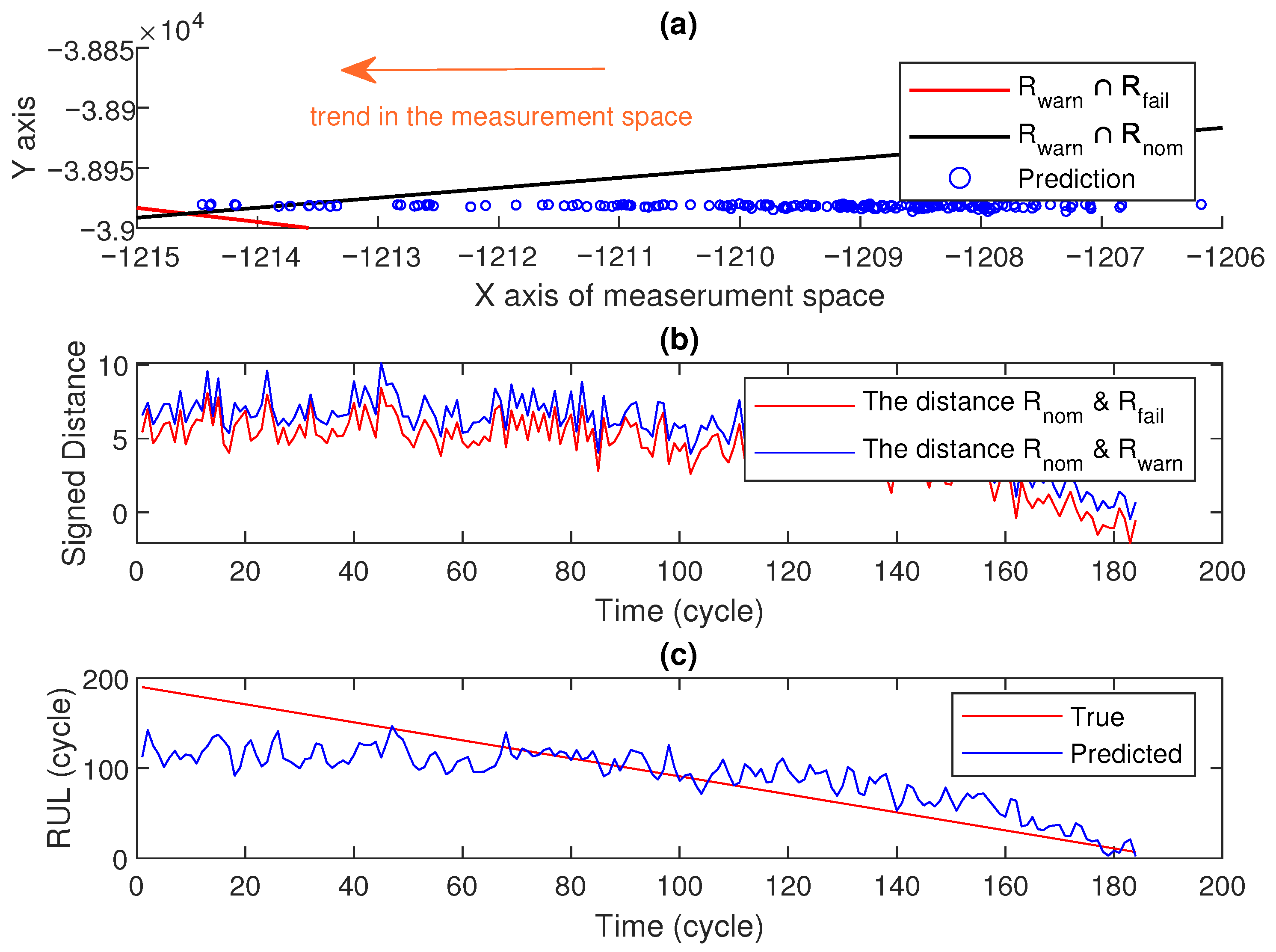
3.6.3. Case Study A: FD002 Engine 7

Key observations:
  • The engine follows a clear left-to-right trajectory in the measurement space, indicating consistent degradation.
  • Distance to the failure boundary decreases monotonically after cycle 200.
  • Final RUL prediction: 2.48 cycles (actual: 6 cycles), yielding a score of 0.31.
  • The warning region is entered at cycle 176, providing 14 cycles of advance warning.
  • Figure 6a shows the trajectory of measurements in the measurement space.
  • Figure 6b displays their distances to the warning and failure boundaries.
  • Figure 6c presents the predicted RUL estimates and true RUL values.

3.6.4. Case Study B: FD001 Engine 1

Engine 1 from FD001 presents a challenging scenario with only 31 available measurements. This case demonstrates the developed framework’s ability to handle limited data:
  • Initial measurements place the unit firmly in the nominal region.
  • A limited degradation trend is observable in the available data.
  • Final RUL prediction: 120.6 cycles (actual: 113 cycles).
  • Despite data scarcity, the prediction error of 6.4 cycles represents a PHM08 score of only 1.38.
  • Figure 7a shows the trajectory of measurements in the measurement space.
  • Figure 7b displays their distances to the warning and failure boundaries.
  • Figure 7c presents the predicted RUL estimates and true RUL values.
This case highlights the robustness of the proposed linear approach when dealing with units in early degradation stages where non-linear methods might overfit to noise.

3.6.5. Overall Performance

Table 2 presents the classification performance through a confusion matrix and F1-scores. The confusion matrix shows the model correctly classified 636 out of 707 samples (90.0% accuracy), with diagonal values of 578, 20, and 38 representing correct predictions for each of the three classes. These results demonstrate that the proposed method maintains classification capabilities across diverse operational conditions while excelling in both regression and classification tasks.
Table 3 compares the proposed method against three conventional approaches (MLP, SVR, and RVR) across four C-MAPSS datasets using RMSE and Score metrics. The performance comparison reveals that the proposed method demonstrates competitive but inconsistent results across the C-MAPSS dataset, while it achieves moderate performance on FD001 (RMSE: 30.40 ) and FD002 (RMSE: 35.40 ), outperforming MLP but falling short of the kernel-based methods (SVR and RVR). The method exhibits significant degradation on FD003 and FD004, particularly evident in the Score metric where it reaches 7.9 × 10 5 and 6.9 × 10 5 , respectively—orders of magnitude worse than the baseline approaches.
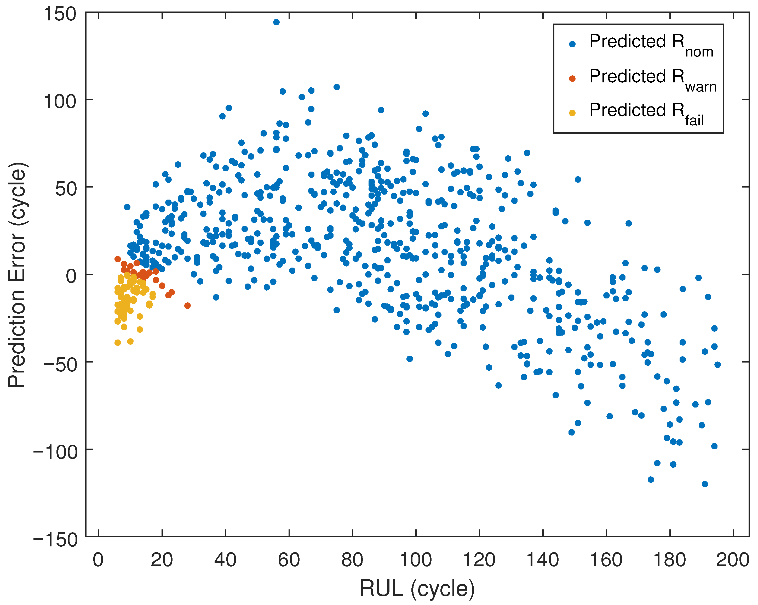
The visualization in Figure 8 presents case-specific RUL cycle values on the horizontal axis, whereas the vertical axis demonstrates the predictive error magnitude relative to the ground-truth RUL values for each case. Moreover, the predicted classes ( R n o m , R w a r n , R f a i l ) are illustrated based on their designated regional boundaries.

4. Conclusions

This paper presents a unified linear framework for predictive maintenance that addresses both classification and regression objectives within a single coherent approach. The proposed method demonstrates that complex predictive maintenance problems can be effectively solved using computationally efficient linear techniques, making it particularly suitable for real-time industrial applications.
The key contributions of this work include the following:
  • A novel integration of LDA for health state classification with distance-based regression for RUL estimation, where the same hyperplane boundaries serve both objectives.
  • A hybrid prediction approach combining linear regression and autoregressive modeling to capture both long-term degradation trends and short-term dynamics.
  • Demonstration that linear methods can achieve competitive performance on the challenging C-MAPSS dataset while maintaining interpretability and computational efficiency.
The experimental results on the NASA C-MAPSS turbofan engine dataset validate the effectiveness of the proposed approach. The framework successfully classifies equipment states into nominal, warning, and failure regions while providing continuous RUL estimates. The case studies demonstrate the method’s robustness, particularly in data-scarce scenarios where only limited operational cycles are available.
The linear nature of the proposed framework offers several practical advantages for industrial deployment:
  • Interpretability: Maintenance engineers can directly understand how sensor measurements influence predictions through the learned hyperplane coefficients.
  • Computational efficiency: Real-time processing capability for monitoring multiple assets simultaneously.
  • Extensibility: Natural accommodation of heterogeneous sensor modalities without complex fusion architectures.
Future work will focus on extending this framework to handle non-monotonic degradation patterns and investigating adaptive boundary learning for evolving operational conditions. Additionally, the approach will be validated on other industrial datasets and we will explore its application to multi-modal sensor fusion scenarios where different sensor types capture complementary aspects of the degradation process.

Author Contributions

Conceptualization, H.A. and U.Y.; methodology, H.A. and U.Y.; software, H.A. and U.Y.; validation, H.A. and U.Y.; formal analysis, H.A. and U.Y.; investigation, H.A. and U.Y.; resources, U.Y.; data curation, H.A. and U.Y.; writing—original draft preparation, H.A. and U.Y.; writing—review and editing, H.A. and U.Y.; visualization, U.Y.; supervision, H.A.; project administration, H.A. and U.Y.; funding acquisition, U.Y. All authors have read and agreed to the published version of the manuscript.

Funding

This work was supported by Adana Science and Technology SRU under project number 24803004.

Data Availability Statement

The C-MAPSS Jet Engine Simulated dataset can be downloaded publicly from its official website.

Conflicts of Interest

The authors declare no conflicts of interest.

Abbreviations

The following abbreviations are used in this manuscript:
RULRemaining Useful Life
LDALinear Discriminant Analysis
ARAutoregressive
RMSERoot Mean Square Error
C-MAPSSCommercial Modular Aero-Propulsion System Simulation
XJTU-SYXi’an Jiaotong University—Suzhou
AICAkaike Information Criterion
SVRSupport Vector Regression
RVRRelevance Vector Regression
MLPsMultilayer Perceptrons

References

  1. Borgi, T.; Hidri, A.; Neef, B.; Naceur, M.S. Data analytics for predictive maintenance of industrial robots. In Proceedings of the 2017 International Conference on Advanced Systems and Electric Technologies (IC_ASET), Hammamet, Tunisia, 14–17 January 2017; pp. 412–417. [Google Scholar]
  2. Biswal, S.; Sabareesh, G.R. Design and development of a wind turbine test rig for condition monitoring studies. In Proceedings of the 2015 International Conference on Industrial Instrumentation and Control (ICIC), Pune, India, 28–30 May 2015; pp. 891–896. [Google Scholar]
  3. Peres, R.S.; Rocha, A.D.; Leitao, P.; Barata, J. IDARTS–towards intelligent data analysis and real-time supervision for industry 4.0. Comput. Ind. 2018, 101, 138–146. [Google Scholar] [CrossRef]
  4. Sezer, E.; Romero, D.; Guedea, F.; Macchi, M.; Emmanouilidis, C. An industry 4.0-enabled low cost predictive maintenance approach for smes. In Proceedings of the 2018 IEEE International Conference on Engineering, Technology and Innovation (ICE/ITMC), Stuttgart, Germany, 17–20 June 2018; pp. 1–8. [Google Scholar]
  5. Nunes, P.; Santos, J.; Rocha, E. Challenges in predictive maintenance–A review. Cirp J. Manuf. Sci. Technol. 2023, 40, 53–67. [Google Scholar] [CrossRef]
  6. Hao, Q.; Xue, Y.; Shen, W.; Jones, B.; Zhu, J. A decision support system for integrating corrective maintenance, preventive maintenance, and condition-based maintenance. In Construction Research Congress 2010: Innovation for Reshaping Construction Practice; American Society of Civil Engineers (ASCE): Reston, VA, USA, 2010; pp. 470–479. [Google Scholar]
  7. Mobley, R.K. An Introduction to Predictive Maintenance; Elsevier: Amsterdam, The Netherlands, 2002. [Google Scholar]
  8. Lee, J.; Kao, H.A.; Yang, S. Service innovation and smart analytics for industry 4.0 and big data environment. Procedia Cirp 2014, 16, 3–8. [Google Scholar] [CrossRef]
  9. Jimenez, J.J.M.; Schwartz, S.; Vingerhoeds, R.; Grabot, B.; Salaün, M. Towards multi-model approaches to predictive maintenance: A systematic literature survey on diagnostics and prognostics. J. Manuf. Syst. 2020, 56, 539–557. [Google Scholar] [CrossRef]
  10. Lei, Y.; Li, N.; Guo, L.; Li, N.; Yan, T.; Lin, J. Machinery health prognostics: A systematic review from data acquisition to RUL prediction. Mech. Syst. Signal Process. 2018, 104, 799–834. [Google Scholar] [CrossRef]
  11. Zhu, J.; Chen, N.; Shen, C. A new multi-task learning framework for remaining useful life prediction. IEEE Trans. Ind. Inform. 2019, 15, 2023–2032. [Google Scholar]
  12. Wang, B.; Lei, Y.; Li, N.; Yan, T. Deep separable convolutional network for remaining useful life prediction of machinery. Mech. Syst. Signal Process. 2020, 134, 106330. [Google Scholar] [CrossRef]
  13. Zhou, L. Multi-task model of adaptive multi-scale feature fusion and adaptive mixture-of-experts for equipment remaining useful life prediction and fault diagnosis. Expert Syst. Appl. 2025, 272, 126807. [Google Scholar] [CrossRef]
  14. Li, R.; Zhan, H.; Yu, J.; Wang, R.; Han, K. A lightweight transformer and depthwise separable convolution model for remaining useful life prediction of turbofan engines. Meas. Sci. Technol. 2024, 35, 025020. [Google Scholar] [CrossRef]
  15. Guo, P.; Liu, Q.; Yu, S.; Xiong, J.; Tan, X.; Guo, C. A transformer with layer-cross decoding for remaining useful life prediction. J. Supercomput. 2023, 79, 11558–11584. [Google Scholar] [CrossRef]
  16. Nunes, P.; Rocha, E.; Santos, J. Adaptive Framework for Maintenance Scheduling Based on Dynamic Preventive Intervals and Remaining Useful Life Estimation. Future Internet 2024, 16, 214. [Google Scholar] [CrossRef]
  17. Wu, F.; Tang, J.; Jiang, Z.; Sun, Y.; Chen, Z.; Guo, B. The Remaining Useful Life Prediction Method of a Hydraulic Pump under Unknown Degradation Model with Limited Data. Sensors 2023, 23, 5931. [Google Scholar] [CrossRef] [PubMed]
  18. Pan, S.-J.; Tsai, M.-L.; Chen, C.-L.; Lin, P.T.; Lee, H.-Y. Investigation of Machine Learning Methods for Predictive Maintenance of the Ultra-High-Pressure Reactor in a Polyethylene-Vinyl Acetate Production Process. Electronics 2023, 12, 580. [Google Scholar] [CrossRef]
  19. Xie, S.; Xue, F.; Zhang, W.; Zhu, J. Data-Driven Predictive Maintenance Policy Based on Dynamic Probability Distribution Prediction of Remaining Useful Life. Machines 2023, 11, 923. [Google Scholar] [CrossRef]
  20. Zhou, S.; Yao, Y.; Liu, A.; Wang, F.; Chen, L.; Xiong, R. Multiform Informed Machine Learning Based on Piecewise and Weibull for Engine Remaining Useful Life Prediction. Sensors 2023, 23, 5669. [Google Scholar] [CrossRef]
  21. Riccio, C.; Menanno, M.; Zennaro, I.; Savino, M.M. A New Methodological Framework for Optimizing Predictive Maintenance Using Machine Learning Combined with Product Quality Parameters. Machines 2024, 12, 443. [Google Scholar] [CrossRef]
  22. Aminzadeh, A.; Sattarpanah Karganroudi, S.; Majidi, S.; Dabompre, C.; Azaiez, K.; Mitride, C.; Sénéchal, E. A Machine Learning Implementation to Predictive Maintenance and Monitoring of Industrial Compressors. Sensors 2025, 25, 1006. [Google Scholar] [CrossRef]
  23. Cen, Z.; Hu, S.; Hou, Y.; Chen, Z.; Ke, Y. Remaining useful life prediction of machinery based on improved Sample Convolution and Interaction Network. Eng. Appl. Artif. Intell. 2024, 135, 108813. [Google Scholar] [CrossRef]
  24. Li, X.; Zhang, Y.; Wang, H.; Liu, J. A method for predicting remaining useful life using enhanced Savitzky–Golay filter and improved deep learning framework. Sci. Rep. 2024, 14, 24123. [Google Scholar] [CrossRef]
  25. Ren, J.; Wang, L.; Zhang, Q.; Chen, M. A novel equipment remaining useful life prediction approach considering dynamic maintenance threshold. Qual. Reliab. Eng. Int. 2024, 40, 1623–1640. [Google Scholar] [CrossRef]
  26. Hamza, R.T. Remaining Useful Life Prediction with Uncertainty Quantification Using Evidential Deep Learning. J. Artif. Intell. Soft Comput. Res. 2025, 15, 43–58. [Google Scholar] [CrossRef]
  27. Qi, D.; Zhu, Z.; Yao, F.; Song, W.; Kudreyko, A.; Cattani, P.; Villecco, F. Predicting the remaining useful life of turbofan engines using fractional Lévy stable motion with long-range dependence. Reliab. Eng. Syst. Saf. 2024, 8, 55. [Google Scholar] [CrossRef]
  28. Liu, L.; Song, X.; Zhou, Z. Aircraft engine remaining useful life estimation via a double attention-based data-driven architecture. Reliab. Eng. Syst. Saf. 2022, 221, 108330. [Google Scholar] [CrossRef]
  29. Costa, N.; Sánchez, L. Variational encoding approach for interpretable assessment of remaining useful life estimation. Reliab. Eng. Syst. Saf. 2022, 222, 108353. [Google Scholar] [CrossRef]
  30. Lillelund, C.M.; Pannullo, F.; Jakobsen, M.O.; Morante, M.; Pedersen, C.F. A probabilistic estimation of remaining useful life from censored time-to-event data. arXiv 2024, arXiv:2405.01614. [Google Scholar]
  31. Chen, L.; Wang, H.; Meng, L.; Xu, Z.; Xue, L.; Ren, M. An End-to-End Adaptive Method for Remaining Useful Life Prediction of Rolling Bearings Using Time–Frequency Image Features. Mach. Learn. Knowl. Extr. 2024, 6, 2892–2912. [Google Scholar] [CrossRef]
  32. Saxena, A.; Goebel, K. PHM08 Challenge Data Set. In NASA Ames Prognostics Data Repository; NASA Ames Research Center: Moffett Field, CA, USA, 2008. Available online: http://ti.arc.nasa.gov/project/prognostic-data-repository (accessed on 10 December 2024).
  33. Maulana, F.; Starr, A.; Ompusunggu, A.P. Explainable Data-Driven Method Combined with Bayesian Filtering for Remaining Useful Lifetime Prediction of Aircraft Engines Using NASA CMAPSS Datasets. Machines 2023, 11, 163. [Google Scholar] [CrossRef]
  34. Drucker, H.; Burges, C.J.; Kaufman, L.; Smola, A.; Vapnik, V. Support vector regression machines. Adv. Neural Inf. Process. Syst. 1996, 9, 155–161. [Google Scholar]
  35. Smola, A.J.; Schölkopf, B. A tutorial on support vector regression. Stat. Comput. 2004, 14, 199–222. [Google Scholar] [CrossRef]
  36. Vapnik, V. Statistical Learning Theory; Wiley-Interscience: Hoboken, NJ, USA, 1998. [Google Scholar]
  37. Tipping, M.E. Sparse Bayesian learning and the relevance vector machine. J. Mach. Learn. Res. 2001, 1, 211–244. [Google Scholar]
  38. Tipping, M.E. The relevance vector machine. In Advances in Neural Information Processing Systems; ACM: New York, NY, USA, 2000; pp. 652–658. [Google Scholar]
  39. Bishop, C.M. Pattern Recognition and Machine Learning; Springer: Berlin/Heidelberg, Germany, 2006. [Google Scholar]
  40. Ramasso, E.; Saxena, A. Performance benchmarking and analysis of prognostic methods for CMAPSS datasets. Int. J. Progn. Health Manag. 2014, 5, 1–15. [Google Scholar] [CrossRef]
  41. Zheng, S.; Ristovski, K.; Farahat, A.; Gupta, C. Long short-term memory network for remaining useful life estimation. In Proceedings of the 2017 IEEE International Conference on Prognostics and Health Management (ICPHM), Dallas, TX, USA, 19–21 June 2017; pp. 88–95. [Google Scholar]
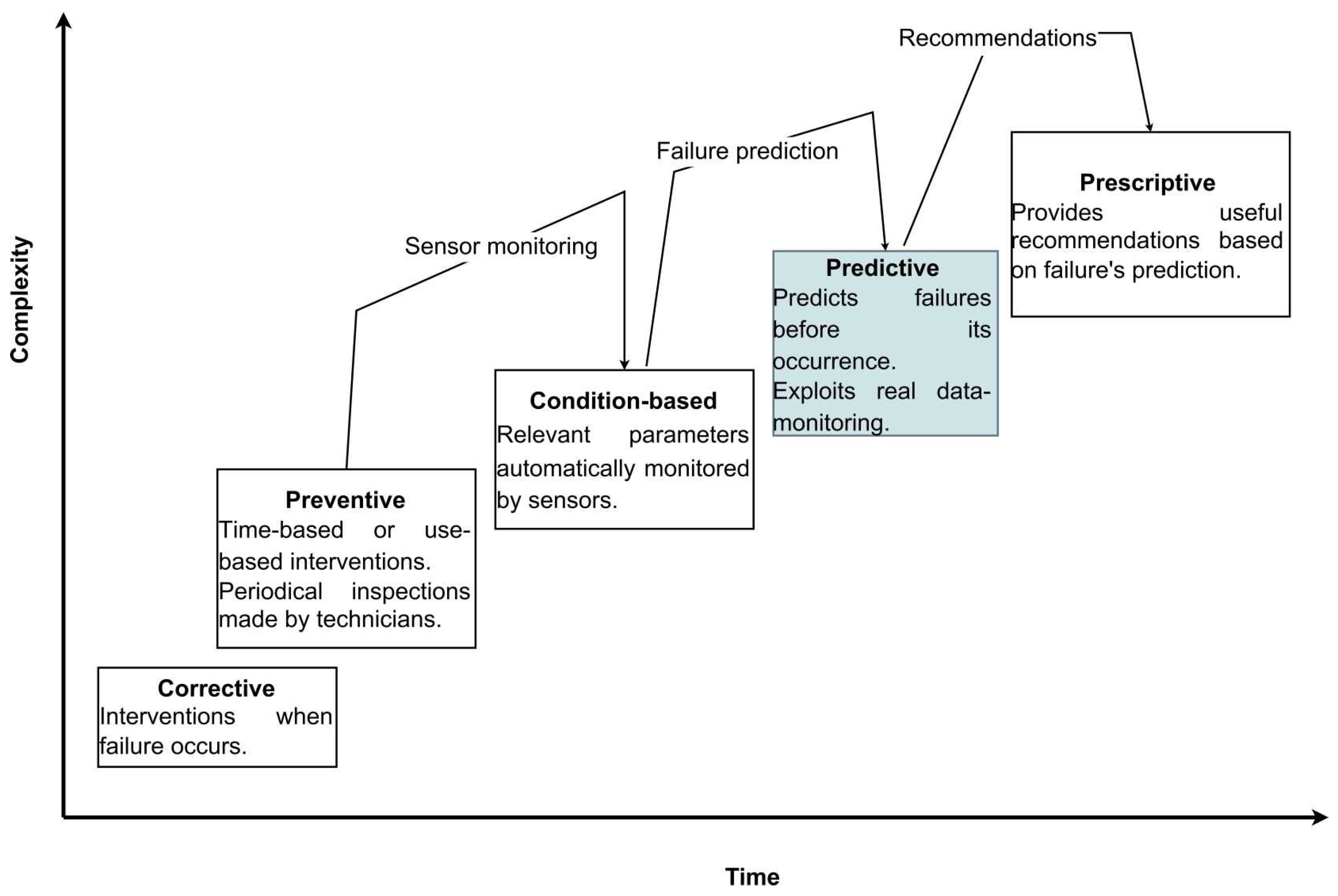
Figure 1. Development of maintenance techniques over time [5].
Applsci 15 09945 g001
Figure 2. Nominal and failure areas in measurement space.
Applsci 15 09945 g002
Figure 3. The proposed linear classification–regression framework for predictive maintenance. The pipeline shows sensor data processing, hyperplane-based classification into health states, distance computation, and RUL estimation through both linear regression and autoregressive time series analysis.
Applsci 15 09945 g003
Figure 4. LDA decision boundaries and class separation in two-dimensional feature space.
Applsci 15 09945 g004
Figure 5. LDA projection with 95% confidence ellipses for multivariate normal assumption validation.
Applsci 15 09945 g005
Figure 6. The performance of the proposed system for engine 7 of FD002.
Applsci 15 09945 g006
Figure 7. The performance of the proposed system for engine 1 of FD001.
Applsci 15 09945 g007
Figure 8. Graphical representation of prediction error and RUL values for each case.
Applsci 15 09945 g008
Table 1. C-MAPSS dataset characteristics.
Dataset
ID
Training
Units
Test
Units
Fault
Mode(s)
Training
Samples
Test
Samples
FD001100100HPC20,63113,096
FD002260259HPC53,75933,991
FD003100100HPC, Fan24,72016,596
FD004249248HPC, Fan61,24941,214
Table 2. Confusion matrix and classification performance scores.
Confusion Matrix
Predicted123
True
157864
2122048
31038
Classification Performance
DatasetF1-microF1-macro
FD0010.9200.678
FD0020.8920.691
FD0030.9200.610
FD0040.8910.640
Combined0.9000.649
Table 3. Performance comparisons of the proposed method and the conventional approaches on the C-MAPSS dataset.
DatasetMetricMethods
MLP [40] SVR [35] RVR [39] Proposed
FD001RMSE 37.56 20.96 23.80 30.40
Score 1.8 × 10 4 1.4 × 10 3 1.5 × 10 3 4.7 × 10 3
FD002RMSE 80.03 42.00 31.30 35.40
Score 7.8 × 10 6 5.9 × 10 5 1.7 × 10 4 3.9 × 10 4
FD003RMSE 37.39 21.05 22.37 45.80
Score 1.7 × 10 4 1.6 × 10 3 1.4 × 10 3 7.9 × 10 5
FD004RMSE 77.37 45.35 34.34 40.3
Score 5.6 × 10 6 3.7 × 10 5 2.7 × 10 4 6.9 × 10 5
Disclaimer/Publisher’s Note: The statements, opinions and data contained in all publications are solely those of the individual author(s) and contributor(s) and not of MDPI and/or the editor(s). MDPI and/or the editor(s) disclaim responsibility for any injury to people or property resulting from any ideas, methods, instructions or products referred to in the content.