Generative Denoising Method for Geological Images with Pseudo-Labeled Non-Matching Datasets

Abstract

Accurate prediction of oil and gas reservoirs requires precise river morphology. However, geological sedimentary images are often degraded by scattered non-structural noise from data errors or printing, which distorts river structures and complicates reservoir interpretation. To address this challenge, we propose GD-PND, a generative framework that leverages pseudo-labeled non-matching datasets to enable geological denoising via information transfer. We first construct a non-matching dataset by deriving pseudo-noiseless images via automated contour delineation and region filling on geological images of varying morphologies, thereby reducing reliance on manual annotation. The proposed style transfer-based generative model for noiseless images employs cyclic training with dual generators and discriminators to transform geological images into outputs with well-preserved river structures. Within the generator, the excitation networks of global features integrated with multi-attention mechanisms can enhance the representation of overall river morphology, enabling preliminary denoising. Furthermore, we develop an iterative denoising enhancement module that performs comprehensive refinement through recursive multi-step pixel transformations and associated post-processing, operating independently of the model. Extensive visualizations confirm intact river courses, while quantitative evaluations show that GD-PND achieves slight improvements, with the chi-squared mean increasing by up to 466.0 (approximately 1.93%), significantly enhancing computational efficiency and demonstrating its superiority.

1. Introduction

Geological modeling technology [1,2,3] has advanced to the intelligent modeling stage [4] where well-described geological model images can be obtained to provide intuitive representations of underground geological structures and sedimentary features, which can offer valuable information for geoscientists in geology, oil exploration, groundwater resource management, and other fields. Notably, these geological images are sometimes disturbed by various types of noise. In Figure 1, images with noise selected from a geological structure model in the Tarim region exhibit numerous scattered points, horizontal and vertical streaks, and interruptions between river courses, resulting from instrument errors or the scarcity and inaccuracy of data. The unclear river morphology and cluttered non-river regions reduce the interpretability of the geological model. Therefore, automatically removing noise from sedimentary images is crucial for subsurface structure prediction.

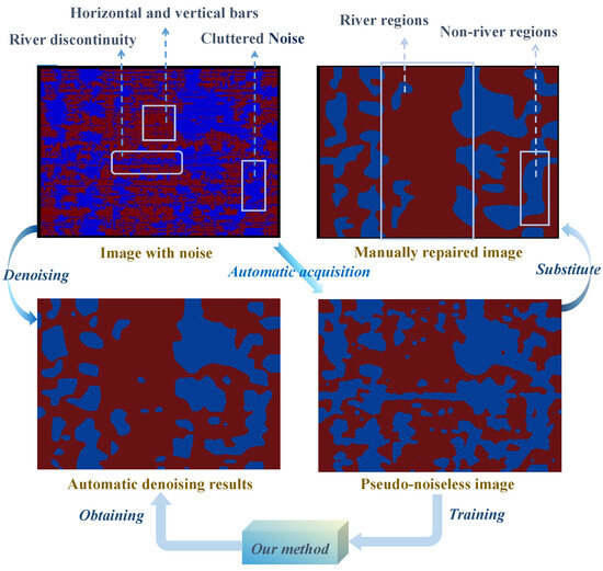
Figure 1. Display of geological images. Horizontal and vertical bars as well as cluttered noise in blue non-river areas are contained. Our method trained on the dataset with pseudo-labels produces results biased toward manually repaired images.

To minimize the introduction of noise in images, many methods aim to obtain high-quality data capable of capturing fine-grained geological structures, thereby ensuring the generation of high-fidelity geological images. Specifically, numerous deep neural network-based methods for reservoir data prediction [5,6], such as Generative Adversarial Networks (GAN) [7], are extensively employed to compensate for incomplete geological data acquisition, which results in missing river regions. Furthermore, advanced intelligent techniques focus on data-level denoising to ensure that high-fidelity data support the reconstruction of complete river structures. In particular, Transformer-based architectures [8] are leveraged to model long-range dependencies and contextual relationships within geological formations, facilitating more accurate restoration of missing or corrupted features [9,10]. Nevertheless, despite the effectiveness of these methods in mitigating scattered noise and missing regions, Figure 1 still exhibits horizontal and vertical streaks caused by printing artifacts, which necessitate image-level denoising to address.

Geological image denoising techniques [11,12] are gaining increasing attention. For sedimentary geological images, early methods typically rely on augmenting a limited set of expert-annotated labels to construct unsupervised anomaly detection networks, where denoising is performed through iterative detection–denoising cycles [13]. However, these methods fail to adequately capture the intrinsic representations of noiseless images, leading to suboptimal denoising outcomes. To overcome this limitation, subsequent studies propose multiscale contrastive learning networks, which leverage contrastive training between annotated and raw images to effectively suppress horizontal and vertical streaks as well as scattered speckle noise around river regions, thereby yielding more faithful representations of channel structures [14]. Notably, these methods require labor-intensive and time-consuming manual annotations, leading to high implementation costs.

In this paper, a generative denoising method for geological images with pseudo-labeled non-matching datasets (GD-PND) is proposed to reduce labor. A non-matching dataset is built with non-river region detection and filling, generating pseudo-noiseless labels instead of manual restoration. The generative model for noiseless images (STGnet) aims to perform style deflection, converting images with noise to noiseless ones by combining cycleGAN with the excitation networks of global features to ensure high-quality generation. Training on non-matching images reduces the requirements for dataset creation, facilitating data expansion. We design an iterative denoising enhancement module (IDEM) to obtain excellent denoising results with smooth boundaries by multiple rounds of contour detection. Numerous visualized results and numerical results fully verify the effectiveness of the overall method and each of its modules.

Related works. Geological modeling [15,16,17] has evolved from traditional two-point [18,19,20] and multi-point statistical methods [21,22,23,24] to intelligent approaches capable of generating high-quality model images [25,26,27]. In particular, generative adversarial networks [7] can produce precise models [28] from large low-redundancy datasets [4], yet the resulting model images still contain scattered non-structural noise that obscures critical geological features, such as river morphology and stratigraphic boundaries. To address this issue, various methods [9,11,13,14,29,30] employ generative frameworks [31,32] to suppress noise. Specifically, GAN [33] can enable the generation of synthetic well-log data that closely approximates real measurements, thereby mitigating noise via data augmentation [30]. Convolutional autoencoder (CAE) [34] can effectively extract features from seismic data by framing reconstruction and denoising as a unified information extraction process, allowing precise signal recovery while attenuating superimposed random noise [29]. Transformer architectures [8] based on self-attention [35] effectively facilitate information exchange across different windows, demonstrating strong performance in suppressing random seismic noise [9]. These data augmentation and denoising methods [36,37,38,39,40] have shown promising results, while noise reduction in geological images [41,42,43,44,45] has recently attracted growing attention. Specifically, the U-net [46] neural networks can eliminate migration artifacts from seismic images to obtain clean images [11]. Unsupervised encoder–decoder–encoder [47] frameworks driven by anomaly detection [48] can eliminate most noise, yet often fail to maintain discontinuities in river courses [13]. The CLGAN method, based on a detect-then-remove strategy, can effectively eliminate noise comprehensively while preserving the continuity of river courses [14]. Nevertheless, a large number of these methods rely on expert-provided annotations, incurring substantial labor and time costs.

2. Research Significance

This study aims to enhance the accuracy of reservoir interpretation, thereby supporting more efficient resource utilization, reducing environmental risks, and promoting sustainable development. The proposed method (GD-PND) aligns with governmental directives and plans on energy security and carbon neutrality, providing a scientific and technological basis for environmentally responsible subsurface exploration and management. The main objective of this research is to mitigate the adverse effects of geological noise on reservoir interpretation through a generative denoising framework, ultimately enabling more reliable decision-making in resource exploration and development.

• Our contributions are summarized as follows:

• We present the generative denoising method for geological images with pseudo-labeled non-matching datasets (GD-PND) to reduce manpower, which takes two types of unpaired images as input to achieve automatic generation and denoising enhancement of noiseless results.
• A non-matching dataset of images with noise and pseudo-noiseless images is built by region detection and filling, overcoming quantity limitations and production difficulties effectively.
• The style transfer-based generative model for noiseless images is created with cycleGAN and excitation networks of global features to achieve high-quality generation from images with noise to noiseless counterparts.
• An iterative denoising enhancement module is designed to obtain better results with smooth boundaries by multiple contour fillings. Extensive experiments are conducted to prove that the model and each of its modules are effective.

3. Materials and Methods

3.1. Method Overview

Our method takes unpaired images with noise and pseudo-noiseless images containing different river morphologies as input. A style transfer-based generative model is utilized to obtain preliminary noise-removed results of geological images, with the incorporation of excitation networks of global features for superior outputs during the transfer process, as described in Section 3.2. Finally, the primary results are improved by multiple outline delineation in an iterative denoising enhancement module, as described in Section 3.4. The pseudo-code of this method is shown in Algorithm 1.

Algorithm 1: Overall process of the GD-PND method.

3.2. The Style Transfer-Based Generative Model

The style transfer-based generative model (STGnet), consisting of two generators and discriminators, performs mutual conversion in two styles between images with noise and generated pseudo-labels without noise in different river morphologies. As shown in Figure 2, small-sized geological images $X_{one}$ with random noise are fed into the generator ($A2B$) to obtain the generated results $X_{genB}$ with river morphology biased toward noiseless images. The pseudo-noiseless images $X_{two}$ are input into the generator ($B2A$) to achieve corresponding generated images with noise $X_{genA}$. Subsequently, results $X_{genB}$ pass through the generator $B2A$ to obtain results $X_{cycleA}$ inclined toward images $X_{one}$, while results $X_{genA}$ are sent into the generator $A2B$ to obtain images $X_{cycleB}$ tending to images $X_{two}$. This process can be expressed as follows:

$$\begin{array}{cc}{X}_{genB}=g_{A2B}\left(X_{one}+{\mathcal{N}}_{ϵ}\right),\hfill & X_{cycleA}=g_{B2A}\left(X_{genB}\right)\approx X_{one}\hfill \\ X_{genA}=g_{B2A}\left(X_{two}\right),\hfill & X_{cycleB}=g_{A2B}\left(X_{genA}\right)\approx X_{two}\hfill \end{array}$$

(1)

where $g_{A2B}\left(\right)$ and $g_{B2A}\left(\right)$ represent the generation process of generators $A2B$ and $B2A$ respectively. ${\mathcal{N}}_{ϵ}$ represents the random noise.

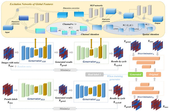
Figure 2. Illustrative overview of the style transfer-based generative model for noiseless images. Generators $A2B$ and $B2A$ realize two types of style transfer between images with noise and images without noise, in which the excitation networks of global features can obtain high-quality feature representation. Discriminators A and B assist the generator for adversarial training.

Then, two discriminators are introduced to respectively accomplish the generation/original discrimination of image sets with noise and image sets without noise. Specifically, images $X_{one}$ and $X_{genA}$ are input as one set to discriminator A for judgment, and images $X_{two}$ and $X_{genB}$ are sent into discriminator B as another set for recognition. The process can be represented as follows:

$$\left[\left({\displaystyle \genfrac{}{}{0pt}{}{scor{e}_{realA}}{scor{e}_{fakeA}}}\right),\left({\displaystyle \genfrac{}{}{0pt}{}{scor{e}_{realB}}{scor{e}_{fakeB}}}\right)\right]=\left(d_A\left(X_{one},X_{genA}\right),d_B\left(X_{two},X_{genB}\right)\right)$$

(2)

where $scor{e}_{realA}$, $scor{e}_{fakeA}$ and $scor{e}_{realB}$, $scor{e}_{fakeB}$ are the judgment probabilities obtained by two discriminators. $d_A\left(\right)$ and $d_B\left(\right)$ are viewed as discriminative processes.

The generators and discriminators in Figure 2 utilize multi-layer convolutional neural networks to extract features, which makes it difficult to ensure high information integrity due to the limitations of representing the global context. To ensure the generation of high-quality denoised images from images with noise, the excitation networks of global features are urgently required to strengthen global features.

Excitation Networks of Global Features

The architecture is shown in Figure 2, in which the input vector ${\mathbf{Z}}_{in}$ undergoes a total of three sub-extraction processes. The vector first passes through a multi-layer perceptron network (${\mathcal{F}}_{MLP}^{\left(1\right)}$) to establish global relationships between features, and the obtained feature is fused with the input by adding to achieve more complete features ${\mathbf{Z}}^{\left(1\right)}$. Subsequently, the channel-wise attention mechanism, which enhances the representational validity and focus between different channels, obtains the vector ${\mathbf{M}}^{\left(ch\right)}$, which is then multiplied with ${\mathbf{Z}}_{in}$ to obtain the output ${\mathbf{Z}}_{first}$. The first sub-process can be expressed as follows:

$$\begin{array}{c}{\mathbf{Z}}^{\left(1\right)}=\alpha ·{\mathcal{F}}_{MLP}^{\left(1\right)}\left({\mathbf{Z}}_{in}\right)\oplus {\mathbf{Z}}_{\mathrm{in}}\hfill \\ {\mathbf{M}}^{\left(ch\right)}={\mathcal{A}}_{ch}\left({\mathbf{Z}}^{\left(1\right)}\right)\hfill \\ {\mathbf{Z}}_{first}={\mathbf{M}}^{\left(ch\right)}\odot {\mathbf{Z}}_{in}\hfill \end{array}$$

(3)

where ${\mathcal{A}}_{ch}$ represents channel attention and $\alpha$ is the determined multiplication coefficient.

After the vector ${\mathbf{Z}}_{first}$ is input into the MLP network again, the obtained feature is added and fused with it by the same coefficient to achieve the output ${\mathbf{Z}}_{mlp}$. Following this, the feature obtained by the spatial attention mechanism (${\mathcal{A}}_{spat}$) that strengthens spatial information focus on ${\mathbf{Z}}_{mlp}$ is fused with the information ${\mathbf{Z}}_{mlp}$ to prevent feature loss. The second sub-process can be expressed as follows:

$${\mathbf{Z}}^{\left(2\right)}={\mathcal{A}}_{spat}\left(\alpha ·{\mathcal{F}}_{MLP}^{\left(2\right)}\left({\mathbf{Z}}_{first}\right)\oplus {\mathbf{Z}}_{first}\right)\odot {\mathbf{Z}}_{mlp}$$

(4)

The third sub-process involves an independent MLP network (${\mathcal{F}}_{MLP}^{\left(3\right)}$) to re-emphasize global semantics, representing the feature processed through ${\mathcal{F}}_{MLP}^{\left(3\right)}$ and fused with the vector ${\mathbf{Z}}^{\left(2\right)}$ to obtain high-quality features ${\mathbf{Z}}^{\left(final\right)}$. The process can be represented as follows:

$${\mathbf{Z}}^{\left(final\right)}={\mathcal{F}}_{MLP}^{\left(3\right)}\left({\mathbf{Z}}^{\left(2\right)}\right)\odot \alpha \oplus {\mathbf{Z}}^{\left(2\right)}$$

(5)

The excitation networks of global features utilize multiple attention and MLP networks to construct a mechanism similar to the Transformer architecture for highly expressive features. Positioned within the encoding and decoding processes of both generators, they extensively focus on global information.

3.3. Training Process of STGnet Model

The proposed model is achieved by adversarial training between generators and discriminators, in which the generator loss includes three parts and the discriminator loss contains two parts, as described in Section 3.3.1 and Section 3.3.2.

3.3.1. Training Losses for the Generator

Initially, the pseudo-noiseless image $X_{two}$ is fed into $A2B$ to obtain the generated image, while the image with noise $X_{one}$ is processed through $B2A$ to obtain the result. When training, the distances between the generated and input images are minimized separately to ensure that both the $A2B$ and $B2A$ generators possess the capability to generate corresponding styles. The loss $los{s}_{gen}$ about style generation can be expressed as follows:

$${\mathcal{L}}_{gen}={\mathbb{E}}_{X_{one}}\left[{∥X_{one}-X_{sameA}∥}_1\right]+{\mathbb{E}}_{X_{two}}\left[{∥X_{two}-X_{sameB}∥}_1\right]$$

(6)

where $X_{sameB}$ and $X_{sameA}$ are the generated results of the two generators $A2B$ and $B2A$ for input $X_{two}$ and $X_{one}$.

The second part is named the loss of style transfer $los{s}_{trans}$, which represents the adversarial loss. The scores $scor{e}_{fakeA}$ and $scor{e}_{fakeB}$ obtained from images $X_{genA}$ and $X_{genB}$ input to the corresponding discriminators are constantly close to the true probability 1. The loss can be represented as follows:

$${\mathcal{L}}_{trans}={∥\left[\begin{array}{c}scor{e}_{fakeA}\hfill \\ scor{e}_{fakeB}\hfill \end{array}\right]-\left[\begin{array}{c}1\hfill \\ 1\hfill \end{array}\right]∥}_2^2$$

(7)

Subsequently, we minimize the distance between the generated image $X_{cycleA}$ and the image with noise $X_{one}$, as well as minimize the distance between image $X_{cycleB}$ and the image $X_{two}$, thereby ensuring that both generators achieve bidirectional style transfer. The third part about the loss of transfer cycle $los{s}_{cycle}$ can be expressed as follows:

$${\mathcal{L}}_{cycle}={\mathbb{E}}_{X_{one}}\left[{∥X_{one}-X_{cycleA}∥}_1\right]+{\mathbb{E}}_{X_{two}}\left[{∥X_{two}-X_{cycleB}∥}_1\right]$$

(8)

The overall loss of the generator $Los{s}_G$ is the sum of the three parts with specific parameters, which is expressed as follows:

$${\mathcal{L}}_G={\mathcal{L}}_{gen}\times \rho +{\mathcal{L}}_{trans}\times \mu +{\mathcal{L}}_{cycle}\times \beta$$

(9)

where $\rho ,\beta ,\mu$ are all fixed parameters used for training.

3.3.2. Training Losses for the Discriminator

The discriminator is trained to assist the generator in producing high-quality results. The discriminator scores $scor{e}_{realA}$ and $scor{e}_{realB}$ for the original inputs gradually approach 1, while the scores $scor{e}_{fakeA}$ and $scor{e}_{fakeB}$ for the generated results continually approach 0. This process can be expressed as follows:

$$\begin{array}{c}{\mathcal{L}}_{dA}=\gamma ·{∥scor{e}_{realA}-1∥}_2^2+\gamma ·{∥scor{e}_{fakeA}-0∥}_2^2\hfill \\ {\mathcal{L}}_{dB}=\gamma ·{∥scor{e}_{realB}-1∥}_2^2+\gamma ·{∥scor{e}_{fakeB}-0∥}_2^2\hfill \end{array}$$

(10)

where ${\mathcal{L}}_{dA}$ and ${\mathcal{L}}_{dB}$ are the losses of two discriminators, and $\gamma$ is the fixed parameter.

3.4. Iterative Denoising Enhancement Module

The results obtained by generator $A2B$ can initially remove a large amount of noise, and the proposed module $IDEM$ achieves more comprehensive noise removal based on these results without the participation of the model. As shown in Figure 3, the module $IDEM$ is divided into two steps. At the beginning, the generated image $X_{genB}$ undergoes the first process of detection to obtain an intermediate image $X_{imm}$. This process includes Gaussian filtering, grayscale conversion, image smoothing, threshold processing, contour detection, and region filling. During this process, grayscale conversion can reduce color information, making the image more concise and clear and facilitating subsequent processing. Filtering and thresholding can reduce image noise and smooth images, thereby highlighting the outline of the target. After applying a color transformation ${\mathcal{T}}_c$ to the river and non-river regions in the image $X_{imm}$, the image is reintroduced into the detection pipeline, following the same procedure but with distinct parameters. Ultimately, the output image undergoes another color transformation to obtain the refined result $X_{first}$ in Figure 3, effectively eliminating a substantial amount of noise from non-river regions.

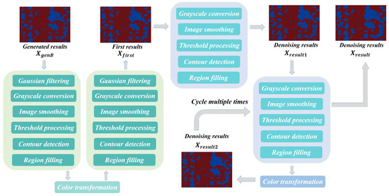
Figure 3. Illustrative overview of the iterative denoising enhancement module. This module adopts the contour detection process to achieve cleanliness in non-river areas, as well as multiple detection and filling processes to achieve denoising in river areas.

The second step is to obtain high-quality denoised images in a cyclic manner. Specifically, the refined result $X_{first}$ undergoes the river-region filling process $\mathcal{R}$ illustrated in Figure 3, where non-river areas are first filled with a designated color. The remaining regions (presumed to be rivers) are then subjected to color transformation, enabling more comprehensive denoising within the river channels. As shown in Figure 3, the resulting image is reintroduced into the same process to produce a progressively improved output. This iterative refinement is repeated multiple times to achieve enhanced denoising performance. The above process can be expressed as follows:

$$\begin{array}{c}{X}_{first}={\mathcal{T}}_c\left({\mathcal{D}}_r\left({\mathcal{T}}_c\left({\mathcal{F}}_{fill}\left({\mathcal{D}}_c\left(X_{genB}\right)\right)\right)\right)\right)\\ X_{final}^{(t+1)}=\mathcal{R}\left(X_{final}^{\left(t\right)}\right),\mathrm{where}{X}_{final}^{\left(0\right)}=X_{first},t=0,1,\dots ,T-1\end{array}$$

(11)

where $X_{final}^{(t+1)}$ and $X_{final}^{\left(t\right)}$ represent the denoising results, and $X_{final}^{\left(t\right)}$ is $X_{first}$ when the number of cycles is 0. ${\mathcal{D}}_c$ and ${\mathcal{D}}_r$ denote the first detection process, including Gaussian filtering, grayscale conversion, image smoothing, thresholding, and contour detection. ${\mathcal{F}}_{fill}$ is the function that fills non-river regions.

4. Results and Discussion

4.1. Experimental Setup

This section comprises three parts. The first part presents the evaluation metric, and the second part explains the procedure for constructing our non-matching dataset. The third part describes the methodological details, including the network architecture and parameter settings.

4.1.1. Evaluation Metric

Several methods are selected for comparing manually restored images ($X_{good}$) with various acquired denoising results. Cosine similarity characterizes image similarity by calculating the cosine distance between vectors. The histogram similarity is calculated by various histogram comparison methods such as correlation coefficient, chi-square comparison, and Bhattacharyya distance ($Bhattach$) method provided by $OpenCV$. Since river courses occupy a major part in geological images, we also set the error rate ($Red-score$) to evaluate its denoising performance. When the same pixel appears red in both images, it is considered to be correctly recovered, and the total count is recorded as $re{d}_{right}$. When a point is red in $X_{good}$ but not red in $X_{result}$, it is considered error recovery, and the total count is recorded as $re{d}_{wrong}$. The error rate can be expressed as follows:

$$Red\text{-}score={\displaystyle \frac{re{d}_{wrong}}{\left.{(red}_{wrong}+re{d}_{right}\right)}}$$

(12)

Wherein, higher cosine similarity and correlation indicate better performance, while lower values are preferable for other evaluation metrics.

4.1.2. Construction of Non-Matching Dataset

The creation process of the non-matching dataset is illustrated in Figure 4. This process primarily consists of two steps: acquiring images with noise $X_{one}$ and obtaining pseudo-noiseless images $X_{two}$.

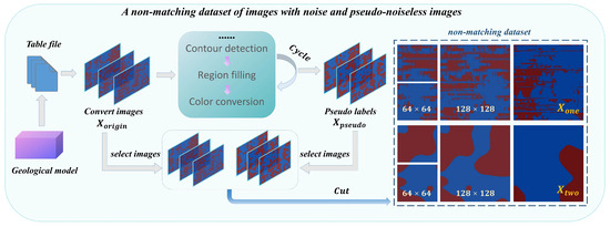
Figure 4. Construction process of the non-matching dataset. Multiple cycles of contour detection and filling are employed to obtain pseudo-noiseless images. Fixed numbers of images with diverse morphologies are segmented at multiple sizes to obtain a large dataset.

Acquiring images with noise: First, a geological model of the Tarim region is converted into a large number of CSV files encoded with 0 and 1, where the 0–1 encoding represents red and blue colors, respectively. Based on the correspondence between color encoding and river courses, each CSV file is automatically transformed into a large-sized image with noise $X_{origin}$, eliminating the need for manual cropping from the models and thereby saving considerable labor. We select 16 images from the original images $X_{origin}$ and divide them into patches of size $64\times 64$ and $128\times 128$, thereby generating a large number of small-sized images with noise $X_{one}$ suitable for training.

Obtaining pseudo-noiseless images: Subsequently, all large-sized images $X_{origin}$ are processed with contour detection, region filling, and color conversion for a total of nine cycles ($cycle=9$) to generate pseudo-labels $X_{pseudo}$, which have been validated by geological experts. Sixteen images with river morphologies different from those previously selected are randomly chosen and divided into patches of size $64\times 64$ and $128\times 128$, producing the pseudo-noiseless images $X_{two}$. The number of non-matching datasets in the two categories is summarized in Table 1.

Table 1. Description of quantities for non-matching dataset.

Size	Images with Noise	Pseudo Labels	Total
$64\times 64$	11,904	11,904	23,808
$128\times 128$	5184	5184	10,368
Total	17,088	17,088	34,176

During this construction process, the implementation of multiple contour detection and region filling has indeed achieved a notable denoising effect. Specifically, the red noises within the non-river regions delineated in Figure 5 are decreasing, especially noticeable from the first cycle to the third cycle of acquisition, which verifies the effectiveness of the method for constructing images $X_{two}$. Notably, the denoising effect after a limited number of cycles is still not as effective as our method (GD-PND), as shown in Figure 6. It is observed that the cosine similarity between the images $X_{pseudo}$ obtained at different cycles and the manually repaired image $X_{good}$ is lower compared to the similarity achieved by our method, which illustrates the necessity of the subsequent method construction in Section 3.

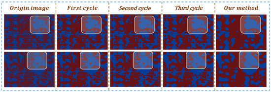
Figure 5. Images $X_{pseudo}$ generated under different cycle times. Although the non-river areas become tidier as the number of iterations increases, the results under limited iterations are still not as good as the denoising results we obtained.

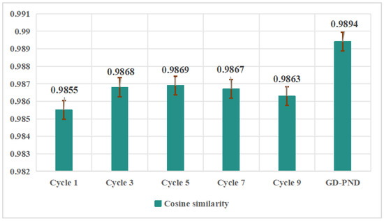
Figure 6. The images $X_{pseudo}$ under different cycles and the results obtained by our method are compared with $X_{good}$ for similarity. The red line is the error bar. Our results show a high degree of similarity.

4.1.3. Methodological Details

The channel attention can be expressed as follows: $Linear\left(\right)\to Relu\left(\right)\to Linear\left(\right)$. The spatial attention can be represented by the following: $Conv\left(\right)\to Batchnorm2d\left(\right)\to Relu\left(\right)\to Conv\left(\right)\to Batchnorm2d\left(\right)$. The MLP network can be represented by the following: $Linear\left(\right)\to Relu\left(\right)\to Linear\left(\right)$. The dimensions of the input and output images are $(32,3,64,64)$. When $cycle=9$ in the dataset, pseudo-labels stop being acquired. Images of size $(774,546)$ are cut into multiple sizes with an interval of 16. The input and output sizes of the two excitation networks of global features are respectively $(32,256,16,16)$ and $(32,64,64,64)$. Parameter $\alpha =0.2$. The residual block in the generator is cycled 5 times. The size of the discriminator output is $(32,1)$. During the training process, $\rho =5$, $\mu =1$, $\beta =10$ and $\gamma =0.5$. The number of training epochs can be set to 70 and each batch to 32. learning rate $lr=0.0001$, and gradient updates are performed by the $Adam$ optimizer. The code is available at https://github.com/Huanzh111/GD-PND (accessed on 23 August 2025).

Our framework is implemented on an NVIDIA RTX 2070 GPU. Owing to the dual-generator and dual-discriminator architecture, each training epoch takes approximately 359 s. During inference, the trained model requires about 0.7789 s to process an input image of size $902\times 635$. Furthermore, the IDEM module takes around 18.19 s to complete 21 iterations.

4.2. Visualization Results of Denoising

Twelve image pairs containing original images with noise and their corresponding denoising results are shown in Figure 7. The proposed method can achieve high-integrity connectivity of river morphologies while ensuring the neatness of other regions. Specifically, the delineated areas of the denoising results in the two columns on the right show clear river contours, distinct morphology, and excellent connectivity of river courses compared to the original images. Many scattered red dots within the blue regions in the last set have been removed, resulting in the clean non-river portion with minor interference from numerous noises. Our method can produce superior denoising results corresponding to diverse morphologies for geological images, thus fully verifying the effectiveness of this method.

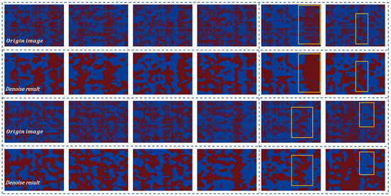
Figure 7. Comparison between denoised results and the original images with noise. The proposed method effectively eliminates numerous noise artifacts, preserving the connectivity of river channels.

Subsequently, the original images with noise and our denoising results are subtracted on the $(R,G,B)$ channel to obtain the distribution results $X_{detect}$ of the noise location, where white represents the noise. As shown in the delineated areas corresponding to Figure 8, our method effectively cleans multi-class noise depicted in Figure 1. Especially noteworthy is the multitude of noise identified within the circled non-river areas and the comprehensive filling of gaps between river courses, ensuring the connectivity of rivers and the cleanliness of the area. Moreover, the high-density identification of horizontal and vertical bars significantly enhances the integrity of the river. In summary, our method achieves superior denoising results for geological images with a large amount of non-structural noise.

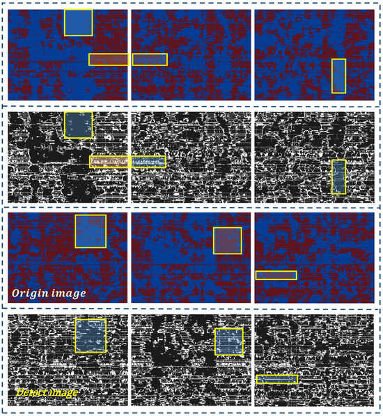
Figure 8. Noise detection results for geological images. The proposed method can remove numerous noises including horizontal and vertical bars, river discontinuities, and cluttered noise.

4.3. Comparative Experiments

To validate the superiority of our method, we compared it with several previously proposed methods mentioned in related works [9,11,14,30,34], as shown in Table 2. Subsequently, we further benchmarked it against denoising methods based on GAN, autoencoder (AE), and CLGAN across various relevant datasets in Table 3, thereby demonstrating both the advantages of our method and the benefits of our datasets.

Table 2. Comparison of average values obtained by different methods on five standards. The results are presented as mean ± standard deviation.

Metrics	CAE	GAN	Unet	CLGAN	Transformer	GD-PND
Cosine Similarity  ↑	0.9880 ± 0.0002	0.9880 ± 0.0001	0.9868 ± 0.0005	0.9879 ± 0.0003	0.9866 ± 0.0003	0.9894 ± 0.0001
Red-score  ↓	0.0859 ± 0.0323	0.0996 ± 0.0084	0.0850 ± 0.0301	0.0753 ± 0.0298	0.0864 ± 0.0484	0.0749 ± 0.0027
Bhattacharyya  ↓	0.1447 ± 0.0038	0.1413 ± 0.0003	0.1444 ± 0.0009	0.1450 ± 0.0021	0.1540 ± 0.0050	0.1409 ± 0.0002
Correlation  ↑	0.9968 ± 0.0027	0.9994 ± 0.0003	0.9970 ± 0.0006	0.9966 ± 0.0014	0.9905 ± 0.0033	0.9998 ± 0.0002
Chi-square  ↓	28,785.4 ± 5135	24,096.3 ± 512.2	28,321.9 ± 1179	29,123.9 ± 2714	40,985.3 ± 6745	23,630.3 ± 253.3

Table 3. Comparison of results obtained by denoising methods under different dataset conditions on five standards. The results are presented as mean ± standard deviation.

Data Conditions	Methods	Correlation ↑	Bhattacharyya ↓	Chi-Square ↓	Cosine Similarity ↑	Red-Score ↓
Only $X_{good}$	CLGAN	0.9655 ± 0.0113	0.1716 ± 0.0062	74,116.9 ± 16,084	0.9823 ± 0.0007	0.2647 ± 0.0316
	GAN	0.9760 ± 0.0156	0.1629 ± 0.0129	62,721.5 ± 13,996	0.9835 ± 0.0012	0.2387 ± 0.0297
	AE	0.9848 ± 0.0064	0.1558 ± 0.0057	46,377.0 ± 9337	0.9844 ± 0.0006	0.2013 ± 0.0238
$X_{good}$ and $X_{noise}$	AE	0.9990 ± 0.0006	0.1417 ± 0.0007	25,347.6 ± 41.84	0.9899 ± 0.0002	0.0907 ± 0.0017
	GAN	0.9954 ± 0.0010	0.1456 ± 0.0011	30,442.9 ± 1609	0.9893 ± 0.0001	0.1149 ± 0.0058
	CLGAN	0.9995 ± 0.0002	0.1413 ± 0.0002	24,062.2 ± 320.7	0.9904 ± 0.0002	0.0790 ± 0.0023
$X_{one}$ and $X_{two}$	Dataset	0.9685 ± 0.0034	0.1694 ± 0.0027	69,863.4 ± 4867	0.9865 ± 0.0002	0.2137 ± 0.0085
	GD-PND	0.9998 ± 0.0002	0.1409 ± 0.0002	23,630.3 ± 253.3	0.9894 ± 0.0001	0.0749 ± 0.0027

4.3.1. Comparison with Other Methods

On our dataset, we conduct multiple experiments for each comparative method and report the average results. As shown in Table 2, our GD-PND method consistently outperforms them in terms of mean performance, which strongly verifies its superiority. In the correlation-related metrics (rows 1, 3–5), our method performs well, indicating its superiority in preserving both overall structure and fine-grained details. In terms of river channel error (second row), it attains the lowest mean value, demonstrating its capability to accurately reconstruct the true river morphology. In contrast, some methods exhibit performance imbalances. For example, GAN and CAE achieve near-optimal correlation but exhibit elevated mean errors (second row), suggesting that while they capture the global structure, they inadequately suppress noise at the fine-detail level, resulting in local distortions and structural deviations. Transformer performs poorly in correlation, as its global modeling capacity does not effectively translate into fine-grained geomorphological representation, limiting its ability to faithfully restore the original river courses. Overall, our results demonstrate both superiority and balance, ensuring consistency in overall river morphology while achieving high-fidelity restoration of fine details.

In Figure 9, a comparison of average inference times highlights the superior efficiency of GD-PND. Specifically, it achieves the shortest mean runtime of 18.97 s, which is approximately 23% faster than GAN (24.85 s) and over 66% faster than U-Net (56.23 s). While Transformer, GAN, and CAE exhibit comparable runtimes of around 24–26 s, CLGAN suffers from higher computational overhead with 34.49 s. These results show that GD-PND not only delivers robust denoising performance but also achieves remarkable computational efficiency, underscoring its practical advantages for real-world applications.

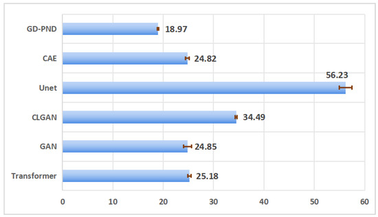
Figure 9. Comparison of inference time among different methods. The horizontal axis is the average time, the vertical axis represents the method, and the red line represents the standard deviation. Our GD-PND method achieves superior performance with shorter average time.

4.3.2. Comparative Experiments on Different Datasets

The results are shown in Table 3, where the data containing $X_{one}$ and $X_{two}$ is our proposed dataset. The dataset $X_{good}$ and $X_{noise}$ cut from manually repaired and manually intercepted images is selected from the paper [14]. Only $X_{good}$ means training using only manually repaired images. Apart from our method, the other methods utilizing $AE$, $GAN$, and $CLGAN$ in the second column for noise detection implement denoising by repeatedly calling the model and modifying pixels.

Compare Methods of Training Only $X_{good}$: As shown in Table 3, our method obviously outperforms those trained solely on $X_{good}$ across all five evaluation metrics, most notably in the chi-square value, which drops significantly from $\mathrm{46,377.0}$ to $\mathrm{23,630.3}$. Compared with our method, these methods exhibit higher error rates when denoising the red rivers, indicating a clear advantage of GD-PND in denoising performance. Besides, both the method trained on $X_{good}$ and our method visualize the images $X_{detect}$ with noise locations and denoised images $X_{result}$ in Figure 10. Our results achieve more complete river morphologies with denser noise detection. Particularly, most of the tiny blue circles within the main river courses in the third row have disappeared compared to the image in the first row. Both the visual and numerical results verify the superiority of our method.

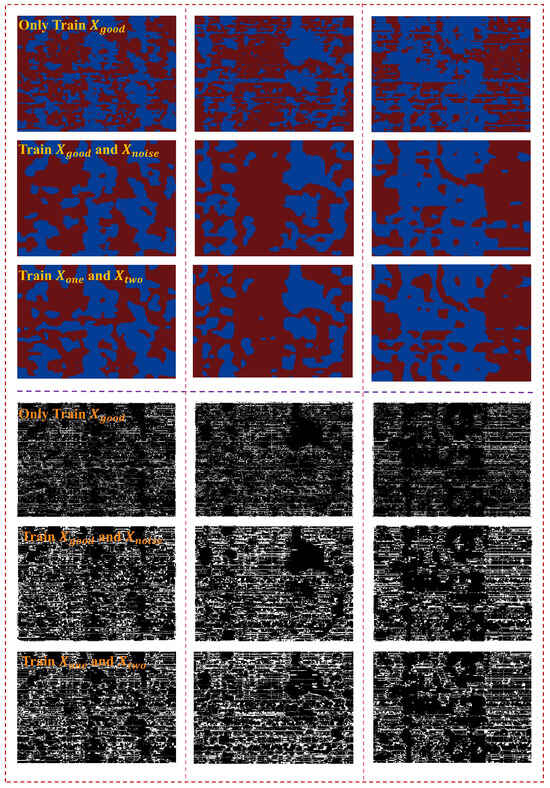
Figure 10. Images $X_{detect}$ (lower part) of noise distribution and denoising results $X_{result}$ (upper part) from various methods. In our denoising results, the river course is relatively complete, and the perceived noise is dense.

Compare Methods of Training $X_{good}$ and $X_{noise}$: The experiments show that our proposed method is not significantly different from the methods implemented on $X_{good}$ and $X_{noise}$ with regard to denoising effects. Specifically, the average results of our method, as shown in Table 3, are similar to those of the method including $CLGAN$, especially in terms of Red-score and correlation, with discrepancies of only 0.41% and 0.03%, respectively. The visual results in Figure 10 indicate that the denoising results for different river morphologies are quite similar, and the perceived noise is densely packed. Notably, our method replaces manual acquisition with automatic label generation, achieving excellent results with less labor, making it more suitable for the field of geological exploration. Moreover, the numerical results for pseudo-noiseless images are inferior to those of the finally acquired denoised images, which highlights the necessity of exploring our method.

4.4. Ablation Experiment

4.4.1. Ablation of Various Modules

Extensive experiments are conducted on different variants in Table 4. ‘without ENGF’ utilizes the remaining processes after removing the excitation networks of global features (ENGF) for denoising. ‘without IDEM’ achieves results from STGnet without the involvement of IDEM and ‘only First’ passes the first step in the IDEM to obtain the results $X_{first}$. In Table 4, our method, GD-PND, shows a significant improvement after feature enhancement, as compared to the result of the variant ‘without ENGF’, proving that more complete feature representation is beneficial to denoising generation. Moreover, most of the results computed by variants without denoising enhancement (without IDEM) or with only one-step denoising enhancement (only First) are inferior to our method (GD-PND), especially in the obvious difference in Chi-square mean from about 30,000 to 23,000, which verifies the importance of module IDEM for denoising. These ablation experiments fully verify the effective performance of important modules in our method.

Table 4. Comparison of multiple variants with different networks or steps across five evaluation criteria. The results are presented as mean ± standard deviation.

Data Conditions	Methods	Correlation ↑	Bhattach ↓	Chi-Square ↓	Cosine Similarity ↑	Red-Score ↓
$X_{one}$ and $X_{two}$	without ENGF	0.9658 ± 0.0024	0.1715 ± 0.0019	73,677.7 ± 3474	0.9859 ± 0.0001	0.2218 ± 0.0054
	without IDEM	0.9920 ± 0.0058	0.1517 ± 0.0084	38,066.8 ± 11,236	0.9882 ± 0.0004	0.0389 ± 0.0225
	only First	0.9964 ± 0.0003	0.1454 ± 0.0003	29,621.9 ± 552.0	0.9881 ± 0.0001	0.0535 ± 0.0022
	GD-PND	0.9998 ± 0.0002	0.1409 ± 0.0002	23,630.3 ± 253.3	0.9894 ± 0.0001	0.0749 ± 0.0027

4.4.2. Visual Analysis of Individual Variants

The visual results of variants are shown in Figure 11. In the absence of excitation networks of global features (ENGFs), the entire denoising process of the IDEM module is superior to only utilizing the first step in this module (only First). It has been observed that the red rivers in the images repaired by IDEM appear more intact, while some unrepaired blue circles are within the rivers obtained from only First. The significance of the overall process of the IDEM module can be reaffirmed by the third group under the STGnet networks, where the IDEM module achieves prominent denoising outcomes with more complete and clearer river courses. Furthermore, the integrity of the STGnet model is important to obtain excellent denoising effects. The second group of images without IDEM shows that the results generated by the entire model exhibit highly intact and connected rivers compared to the results obtained by part of the network, thus emphasizing the superiority of STGnet.

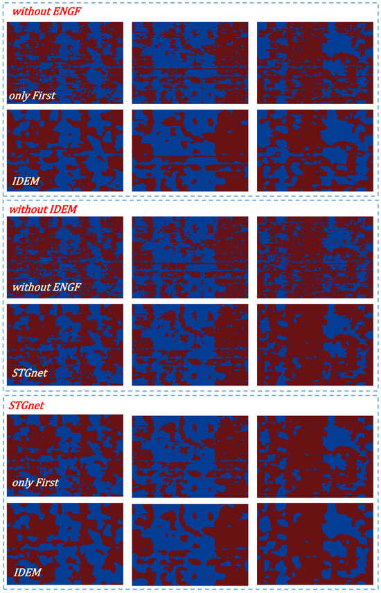
Figure 11. Visualized results of denoising under different variants. Our method achieves superior denoising results.

4.4.3. Ablation on Small Pieces of the Network

Ablation experiments are performed on the excitation networks of global features for different combinations, as shown in Table 5. The average results obtained from generation methods, including only channel attention (only CA + IDEM) or spatial attention (only SA + IDEM), are both inferior to the results obtained from our GD-PND. Moreover, the average results from generation models combining both types of attention (SA + CA + IDEM) are still not as good as those from STGnet, which incorporates the entire excitation networks of global features, which illustrates the excellence of the proposed networks. Additionally, there exists a progressive relationship among the average results obtained without IDEM (SA+CA), using only a single-step denoising (SA + CA + first), and using the entire IDEM (SA + CA + IDEM), validating the excellence of the constructed IDEM module.

Table 5. Experiments on small pieces of the network.

Methods	Correlation	Bhattacharyya	Chi-Square
SA + CA	0.9809 ± 0.0023	0.1686 ± 0.0036	60,662.7 ± 4884
SA + CA + first	0.9836 ± 0.0042	0.1644 ± 0.0066	54,959.2 ± 8945
only SA + IDEM	0.9874 ± 0.0006	0.1534 ± 0.0006	42,463.6 ± 941.0
only CA + first	0.9974 ± 0.0003	0.1440 ± 0.0003	27,807.3 ± 490.7
only CA + IDEM	0.9995 ± 0.0001	0.1411 ± 0.0001	23,918.1 ± 116.7
SA + CA + IDEM	0.9909 ± 0.0005	0.1533 ± 0.0007	40,040.3 ± 915.9
GD-PND	0.9998 ± 0.0002	0.1409 ± 0.0002	23,630.3 ± 253.3

5. Conclusions

To achieve light-labor automatic denoising of geological images, we propose a generative denoising method for geological images using pseudo-labeled non-matching datasets(GD-PND). We construct a non-matching dataset containing images with noise and pseudo-noiseless images generated automatically by contouring and filling processes, thereby reducing manual labor costs associated with repairing images. Subsequently, the style transfer-based generative model for noiseless images (STGnet) aims at transforming images with noise into noiseless counterparts, thereby directly generating denoised geological images. Additionally, we design an iterative denoising enhancement module (IDEM), which applies boundary detection and area filling multiple times to achieve superior denoising results. Extensive visual and numerical analyses are provided to demonstrate the efficacy of our proposed method.

Nevertheless, this study has several limitations. First, the pseudo-labeling process may introduce bias or propagate errors, which can potentially affect denoising quality in some cases. Second, while the proposed framework can generate well-described geological images that support 3D model construction, the intermediate processing steps are still relatively complex and could be further refined. Developing a more direct approach for denoising 3D data without converting it into 2D images should be considered. In the future, we will focus on addressing these limitations by improving the reliability of pseudo-label generation and extending the framework to large-scale 3D models.

References

- Chen, Q.; Liu, G.; He, Z.; Zhang, X.; Wu, C. Current situation and prospect of structure-attribute integrated 3D geological modeling technology for geological big data. Bull. Geol. Sci. Technol. 2020, 39, 51–58. [Google Scholar]
- Feng, R.; Grana, D.; Mukerji, T.; Mosegaard, K. Application of Bayesian generative adversarial networks to geological facies modeling. Math. Geosci. 2022, 54, 831–855. [Google Scholar] [CrossRef]
- Bi, Z.; Wu, X. Implicit structural modeling of geological structures with deep learning. In Proceedings of the First International Meeting for Applied Geoscience & Energy, Denver, CO, USA, 26 September–1 October 2021. [Google Scholar]
- Liu, Y.; Zhang, W.; Duan, T.; Lian, P.; Li, M.; Zhao, H. Progress of deep learning in oil and gas reservoir geological modeling. Bull. Geol. Sci. Technol. 2021, 40, 235–241. [Google Scholar]
- Li, J.; Meng, Y.; Xia, J.; Xu, K.; Sun, J. A Physics-Constrained Two-Stage GAN for Reservoir Data Generation: Enhancing Predictive Accuracy. Eng. Res. Express 2025, 7, 035257. [Google Scholar] [CrossRef]
- Huang, W.; Wang, Y.; Wang, P.; Tu, Z.; Kong, X.; Luo, Y.; Jia, Y.; Zhao, Z.; Hu, X. Dual-driven gas reservoir productivity prediction with small sample data: Integrating physical constraints and GAN-based data augmentation. Geoenergy Sci. Eng. 2025, 247, 213711. [Google Scholar] [CrossRef]
- Goodfellow, I.; Pouget-Abadie, J.; Mirza, M.; Xu, B.; Warde-Farley, D.; Ozair, S.; Courville, A.; Bengio, Y. Generative adversarial nets. arXiv 2014, arXiv:1406.2661. [Google Scholar] [CrossRef]
- Liu, Z.; Lin, Y.; Cao, Y.; Hu, H.; Wei, Y.; Zhang, Z.; Lin, S.; Guo, B. Swin transformer: Hierarchical vision transformer using shifted windows. In Proceedings of the IEEE/CVF International Conference on Computer Vision, Virtually, 11–17 October 2021; pp. 10012–10022. [Google Scholar]
- Li, F.; Liu, H.; Wang, W.; Ma, J. Swin transformer for seismic denoising. IEEE Geosci. Remote Sens. Lett. 2024, 21, 7501905. [Google Scholar] [CrossRef]
- Wang, H.; Lin, J.; Li, Y.; Dong, X.; Tong, X.; Lu, S. Self-supervised pretraining transformer for seismic data denoising. IEEE Trans. Geosci. Remote Sens. 2024, 62, 5907525. [Google Scholar] [CrossRef]
- Klochikhina, E.; Crawley, S.; Chemingui, N. Seismic image denoising with convolutional neural network. In Proceedings of the SEG International Exposition and Annual Meeting, Denver, CO, USA, 26 September–1 October 2021; SEG: Houston, TX, USA, 2021; p. D011S124R005. [Google Scholar]
- Li, J.; Wu, X.; Hu, Z. Deep learning for simultaneous seismic image super-resolution and denoising. IEEE Trans. Geosci. Remote Sens. 2021, 60, 5901611. [Google Scholar]
- Zhang, H.; Wu, C.; Lu, J.; Wang, L.; Hu, F.; Zhang, L. An Unsupervised Automatic Denoising Method Based on Visual Features of Geological Images. CN202211291834.3, 20 January 2023. [Google Scholar]
- Wu, C.; Zhang, H.; Wang, B.; Zhang, L.; Wang, L.; Hu, F. Multiscale Contrastive Learning Networks for Automatic Denoising of Geological Sedimentary Model Images. IEEE Trans. Geosci. Remote Sens. 2022, 60, 4709212. [Google Scholar] [CrossRef]
- Huo, C.; Gu, L.; Zhao, C.; Yan, W.; Yang, Q. Integrated reservoir geological modeling based on seismic, log and geological data. Acta Pet. Sin. 2007, 28, 66. [Google Scholar]
- Wu, S.; Li, Y. Reservoir modeling: Current situation and development prospect. Mar. Orig. Pet. Geol. 2007, 12, 53–60. [Google Scholar]
- Jia, A.; Guo, Z.; Guo, J.; Yan, H. Research achievements on reservoir geological modeling of China in the past three decades. Acta Pet. Sin. 2021, 42, 1506. [Google Scholar]
- Oliver, M.A.; Webster, R. Basic Steps in Geostatistics: The Variogram and Kriging; Technical report; Springer: Cham, Switzerland, 2015. [Google Scholar]
- Liu, C.; Wang, B.; Yang, G. Rock Mass Wave Velocity Visualization Model Based on the Ordinary Kriging Method. Soil Eng. Found. 2017, 31, 6. [Google Scholar]
- Abulkhair, S.; Madani, N. Stochastic modeling of iron in coal seams using two-point and multiple-point geostatistics: A case study. Mining, Metall. Explor. 2022, 39, 1313–1331. [Google Scholar] [CrossRef]
- Liu, Y. Using the Snesim program for multiple-point statistical simulation. Comput. Geosci. 2006, 32, 1544–1563. [Google Scholar] [CrossRef]
- Zhang, T.; Switzer, P.; Journel, A. Filter-based classification of training image patterns for spatial simulation. Math. Geol. 2006, 38, 63–80. [Google Scholar] [CrossRef]
- Zhang, T.; Xie, J.; Hu, X.; Wang, S.; Yin, J.; Wang, S. Multi-Point Geostatistical Sedimentary Facies Modeling Based on Three-Dimensional Training Images. Glob. J. Earth Sci. Eng. 2020, 7, 37–53. [Google Scholar] [CrossRef]
- Ba, N.T.; Quang, T.P.H.; Bao, M.L.; Thang, L.P. Applying multi-point statistical methods to build the facies model for Oligocene formation, X oil field, Cuu Long basin. J. Pet. Explor. Prod. Technol. 2019, 9, 1633–1650. [Google Scholar] [CrossRef]
- Song, S.; Mukerji, T.; Hou, J. Geological Facies modeling based on progressive growing of generative adversarial networks (GANs). Comput. Geosci. 2021, 25, 1251–1273. [Google Scholar] [CrossRef]
- Bai, T.; Tahmasebi, P. Hybrid geological modeling: Combining machine learning and multiple-point statistics. Comput. Geosci. 2020, 142, 104519. [Google Scholar] [CrossRef]
- Zhang, T.F.; Tilke, P.; Dupont, E.; Zhu, L.C.; Liang, L.; Bailey, W. Generating geologically realistic 3D reservoir facies models using deep learning of sedimentary architecture with generative adversarial networks. Pet. Sci. 2019, 16, 541–549. [Google Scholar] [CrossRef]
- Zhang, C.; Song, X.; Azevedo, L. U-net generative adversarial network for subsurface facies modeling. Comput. Geosci. 2021, 25, 553–573. [Google Scholar] [CrossRef]
- Jiang, J.; Ren, H.; Zhang, M. A convolutional autoencoder method for simultaneous seismic data reconstruction and denoising. IEEE Geosci. Remote Sens. Lett. 2021, 19, 1–5. [Google Scholar] [CrossRef]
- Al-Fakih, A.; Kaka, S.; Koeshidayatullah, A. Utilizing GANs for Synthetic Well Logging Data Generation: A Step Towards Revolutionizing Near-Field Exploration. In Proceedings of the EAGE/AAPG Workshop on New Discoveries in Mature Basins. European Association of Geoscientists & Engineers, Kuala Lumpur, Malaysia, 30–31 January 2024; Volume 2024, pp. 1–5. [Google Scholar]
- Al-Fakih, A.; Koeshidayatullah, A.; Mukerji, T.; Al-Azani, S.; Kaka, S.I. Well log data generation and imputation using sequence based generative adversarial networks. Sci. Rep. 2025, 15, 11000. [Google Scholar] [CrossRef]
- Azevedo, L.; Paneiro, G.; Santos, A.; Soares, A. Generative adversarial network as a stochastic subsurface model reconstruction. Comput. Geosci. 2020, 24, 1673–1692. [Google Scholar] [CrossRef]
- Garcia, L.G.; Ramos, G.D.O.; de Oliveira, J.M.M.T.; Da Silveira, A.S. Enhancing Synthetic Well Logs with PCA-Based GAN Models. In Proceedings of the 2024 International Conference on Machine Learning and Applications (ICMLA), Miami, FL, USA, 18–20 December 2024; IEEE: Miami, FL, USA, 2024; pp. 1350–1355. [Google Scholar]
- Masci, J.; Meier, U.; Cireşan, D.; Schmidhuber, J. Stacked convolutional auto-encoders for hierarchical feature extraction. In Proceedings of the Artificial Neural Networks and Machine Learning–ICANN 2011: 21st International Conference on Artificial Neural Networks, Espoo, Finland, 14–17 June 2011; Proceedings, Part I 21. Springer: Berlin/Heidelberg, Germany, 2011; pp. 52–59. [Google Scholar]
- Pan, X.; Ge, C.; Lu, R.; Song, S.; Chen, G.; Huang, Z.; Huang, G. On the integration of self-attention and convolution. In Proceedings of the IEEE/CVF Conference on Computer Vision and Pattern Recognition, New Orleans, LA, USA, 18–24 June 2022; pp. 815–825. [Google Scholar]
- Li, S.; Chen, J.; Xiang, J. Applications of deep convolutional neural networks in prospecting prediction based on two-dimensional geological big data. Neural Comput. Appl. 2020, 32, 2037–2053. [Google Scholar] [CrossRef]
- Das, V.; Mukerji, T. Petrophysical properties prediction from prestack seismic data using convolutional neural networks. Geophysics 2020, 85, N41–N55. [Google Scholar] [CrossRef]
- Wang, J.; Cao, J. Deep learning reservoir porosity prediction using integrated neural network. Arab. J. Sci. Eng. 2022, 47, 11313–11327. [Google Scholar] [CrossRef]
- Chen, G.; Liu, Y.; Zhang, M.; Zhang, H. Dropout-Based Robust Self-Supervised Deep Learning for Seismic Data Denoising. IEEE Geosci. Remote Sens. Lett. 2022, 19, 8027205. [Google Scholar] [CrossRef]
- Sang, W.; Yuan, S.; Yong, X.; Jiao, X.; Wang, S. DCNNs-based denoising with a novel data generation for multidimensional geological structures learning. IEEE Geosci. Remote Sens. Lett. 2020, 18, 1861–1865. [Google Scholar] [CrossRef]
- Du, H.; An, Y.; Ye, Q.; Guo, J.; Liu, L.; Zhu, D.; Childs, C.; Walsh, J.; Dong, R. Disentangling noise patterns from seismic images: Noise reduction and style transfer. IEEE Trans. Geosci. Remote Sens. 2022, 60, 4513214. [Google Scholar] [CrossRef]
- Zhang, H.; Wang, W. Imaging Domain Seismic Denoising Based on Conditional Generative Adversarial Networks (CGANs). Energies 2022, 15, 6569. [Google Scholar] [CrossRef]
- Zhang, Y.; Lin, H.; Li, Y.; Ma, H. A patch based denoising method using deep convolutional neural network for seismic image. IEEE Access 2019, 7, 156883–156894. [Google Scholar] [CrossRef]
- Liu, G.; Liu, Y.; Li, C.; Chen, X. Weighted multisteps adaptive autoregression for seismic image denoising. IEEE Geosci. Remote Sens. Lett. 2018, 15, 1342–1346. [Google Scholar] [CrossRef]
- Zhang, Y.; Lin, H.; Li, Y. Noise attenuation for seismic image using a deep residual learning. In Proceedings of the SEG Technical Program Expanded Abstracts 2018, Anaheim, CA, USA, 14–19 October 2018; Society of Exploration Geophysicists: Houston, TX, USA, 2018; pp. 2176–2180. [Google Scholar]
- Ronneberger, O.; Fischer, P.; Brox, T. U-net: Convolutional networks for biomedical image segmentation. In Proceedings of the Medical Image Computing and Computer-Assisted Intervention–MICCAI 2015: 18th International Conference, Munich, Germany, 5–9 October 2015; Proceedings, Part III 18. Springer: Cham, Switzerland, 2015; pp. 234–241. [Google Scholar]
- Akcay, S.; Atapour-Abarghouei, A.; Breckon, T.P. Ganomaly: Semi-supervised anomaly detection via adversarial training. In Proceedings of the Asian Conference on Computer Vision, Perth, Australia, 2–6 December 2018; Springer: Cham, Switzerland, 2018; pp. 622–637. [Google Scholar]
- Xia, X.; Pan, X.; Li, N.; He, X.; Ma, L.; Zhang, X.; Ding, N. GAN-based anomaly detection: A review. Neurocomputing 2022, 493, 497–535. [Google Scholar] [CrossRef]
Disclaimer/Publisher’s Note: The statements, opinions and data contained in all publications are solely those of the individual author(s) and contributor(s) and not of MDPI and/or the editor(s). MDPI and/or the editor(s) disclaim responsibility for any injury to people or property resulting from any ideas, methods, instructions or products referred to in the content. |
© 2025 by the authors. Licensee MDPI, Basel, Switzerland. This article is an open access article distributed under the terms and conditions of the Creative Commons Attribution (CC BY) license (https://creativecommons.org/licenses/by/4.0/).