Figure 1.
Fritillariae Thunbergii Bulbus.
Figure 1.
Fritillariae Thunbergii Bulbus.
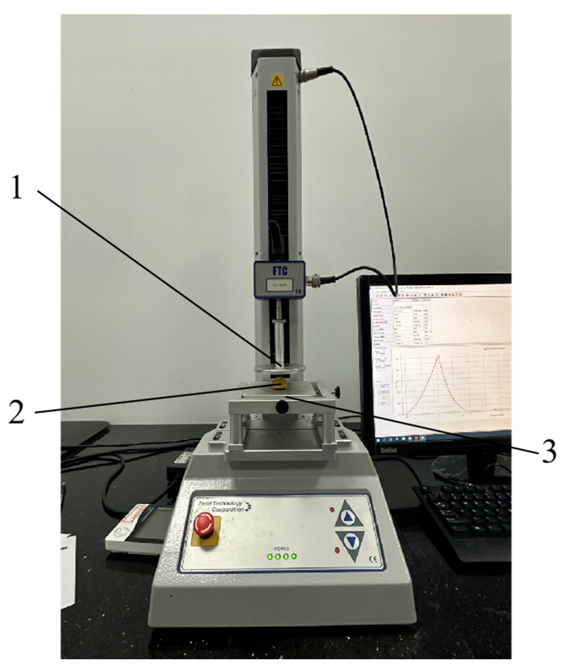
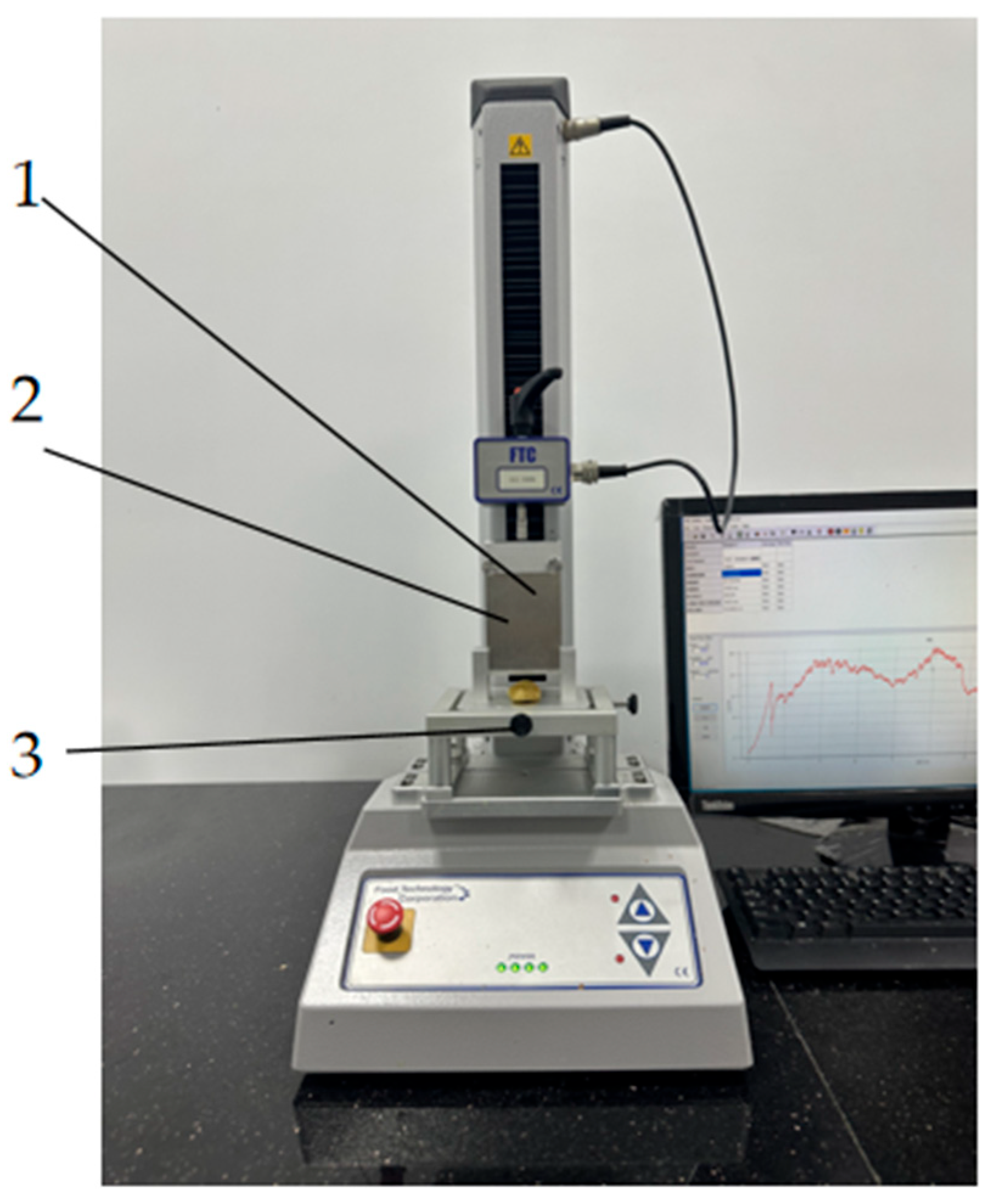
Figure 2.
Uniaxial compression test. 1. Flat probe. 2. FTB sample. 3. Base platform.
Figure 2.
Uniaxial compression test. 1. Flat probe. 2. FTB sample. 3. Base platform.
Figure 3.
Static friction test of FTB. (a) Friction test between FTB and the stainless steel plate; (b) friction test of FTB with industrial rubber. 1. Friction testing apparatus. 2. High-speed camera. 3. FTB sample. 4. Protractor. 5. Stainless steel plate. 6. Industrial rubber.
Figure 3.
Static friction test of FTB. (a) Friction test between FTB and the stainless steel plate; (b) friction test of FTB with industrial rubber. 1. Friction testing apparatus. 2. High-speed camera. 3. FTB sample. 4. Protractor. 5. Stainless steel plate. 6. Industrial rubber.
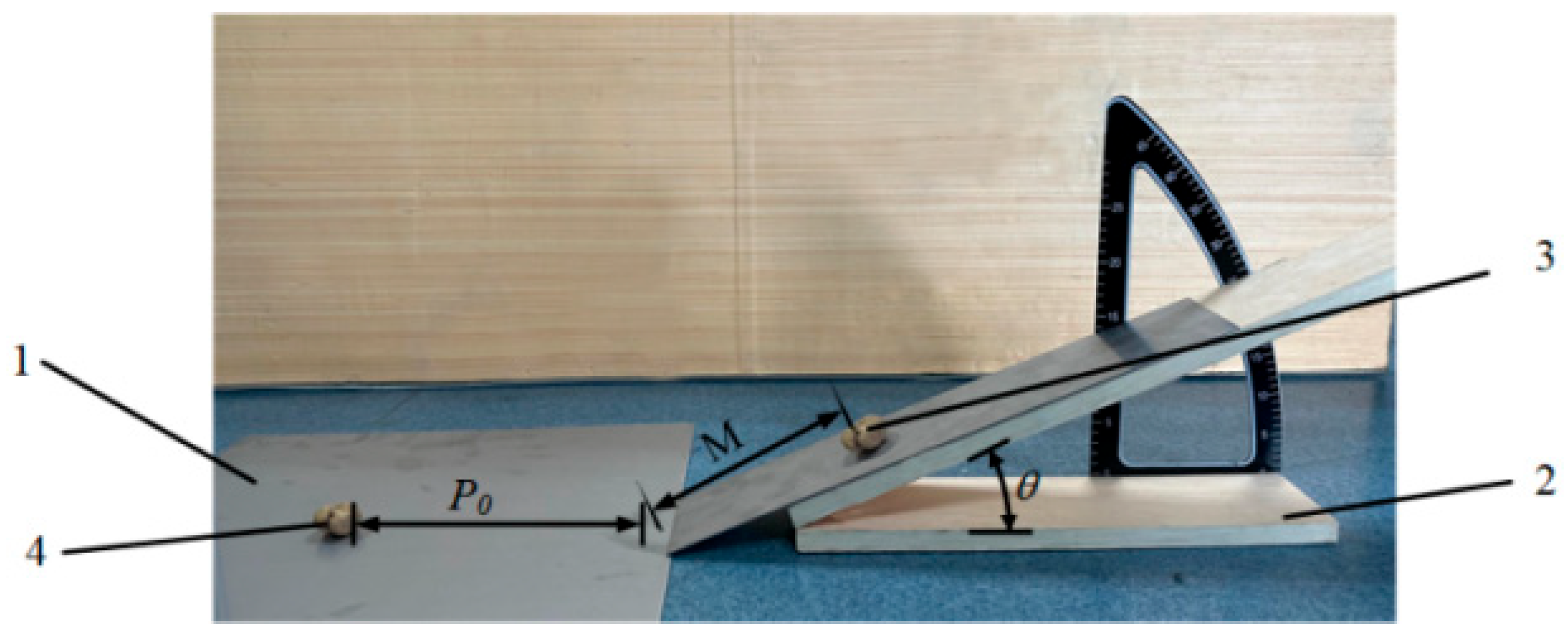
Figure 4.
Rolling friction test of FTB. 1. Stainless steel plate. 2. Friction apparatus. 3. Initial position of the FTB sample. 4. Final resting position of the FTB sample after rolling.
Figure 4.
Rolling friction test of FTB. 1. Stainless steel plate. 2. Friction apparatus. 3. Initial position of the FTB sample. 4. Final resting position of the FTB sample after rolling.
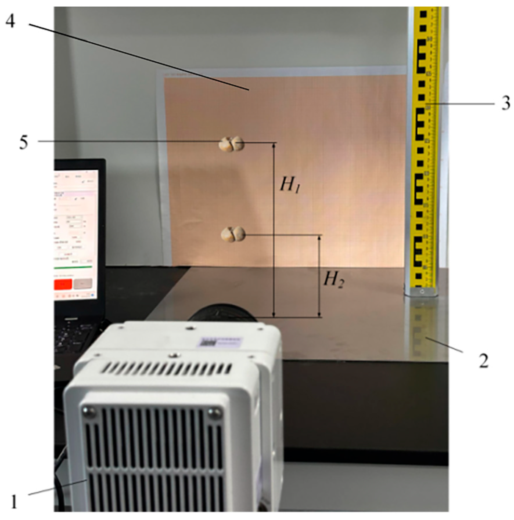
Figure 5.
Collision test between FTB and the stainless steel plate. 1. High-speed camera. 2. Stainless steel plate. 3. Calibration ruler. 4. Coordinate paper. 5. FTB samples.
Figure 5.
Collision test between FTB and the stainless steel plate. 1. High-speed camera. 2. Stainless steel plate. 3. Calibration ruler. 4. Coordinate paper. 5. FTB samples.
Figure 6.
Collision test between the FTB samples themselves. (a) Initial state; (b) maximum swing after collision. 1. High-speed camera. 2. Coordinate paper. 3. FTB samples. 4. Suspension thread.
Figure 6.
Collision test between the FTB samples themselves. (a) Initial state; (b) maximum swing after collision. 1. High-speed camera. 2. Coordinate paper. 3. FTB samples. 4. Suspension thread.
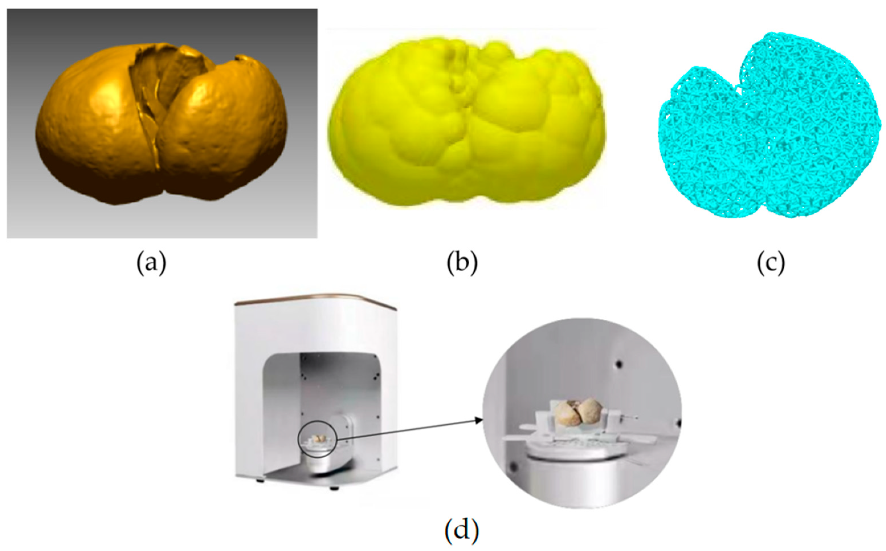
Figure 7.
Simulation model of discrete elements of FTB and the 3D scanner. (a) A 3D scanning model. (b) Discrete element filling model. (c) Bonding key model. (d) K500 automatic turntable 3D scanner.
Figure 7.
Simulation model of discrete elements of FTB and the 3D scanner. (a) A 3D scanning model. (b) Discrete element filling model. (c) Bonding key model. (d) K500 automatic turntable 3D scanner.
Figure 8.
Shear test of FTB. 1. Shear blade. 2. FTB sample. 3. Base platform.
Figure 8.
Shear test of FTB. 1. Shear blade. 2. FTB sample. 3. Base platform.
Figure 9.
Results of single-factor experiments. Note: x1 is the particle contact radius, x2 is the normal stiffness per unit area, x3 is the tangential stiffness per unit area, x4 is the critical normal stress, x5 is the critical tangential stress, and x6 is the bonding radius.
Figure 9.
Results of single-factor experiments. Note: x1 is the particle contact radius, x2 is the normal stiffness per unit area, x3 is the tangential stiffness per unit area, x4 is the critical normal stress, x5 is the critical tangential stress, and x6 is the bonding radius.
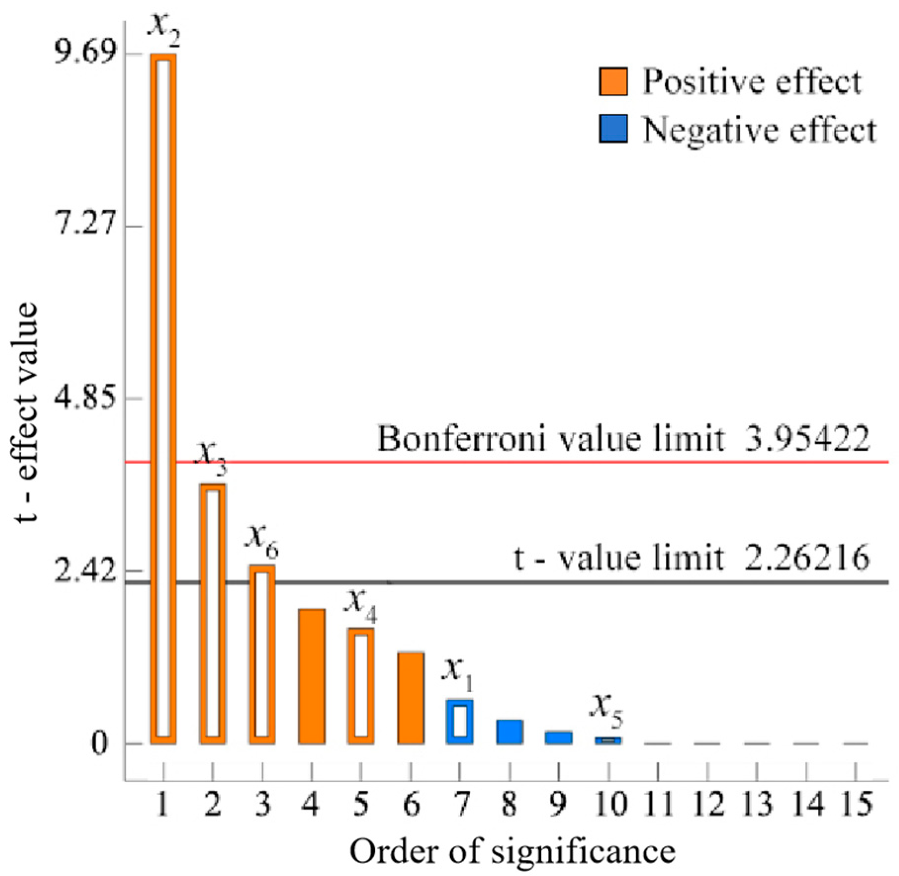
Figure 10.
Pareto chart for a two-level factorial experiment. Note: x1 is the particle contact radius, x2 is the normal stiffness per unit area, x3 is the tangential stiffness per unit area, x4 is the critical normal stress, x5 is the critical tangential stress, and x6 is the bonding radius. The empty square columns in the figure represent six influencing factors.
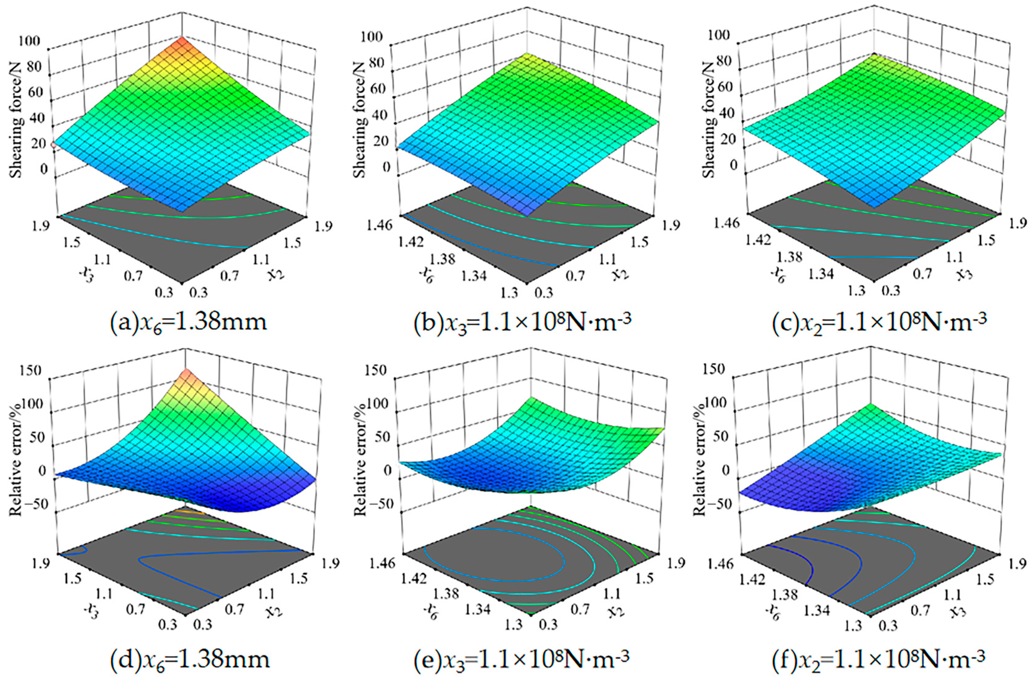
Figure 11.
Significant interaction factor response surface plot to maximum shear force and relative error. Note: x2 is the normal stiffness per unit area, x3 is the tangential stiffness per unit area, and x6 is the bonding radius.
Figure 11.
Significant interaction factor response surface plot to maximum shear force and relative error. Note: x2 is the normal stiffness per unit area, x3 is the tangential stiffness per unit area, and x6 is the bonding radius.
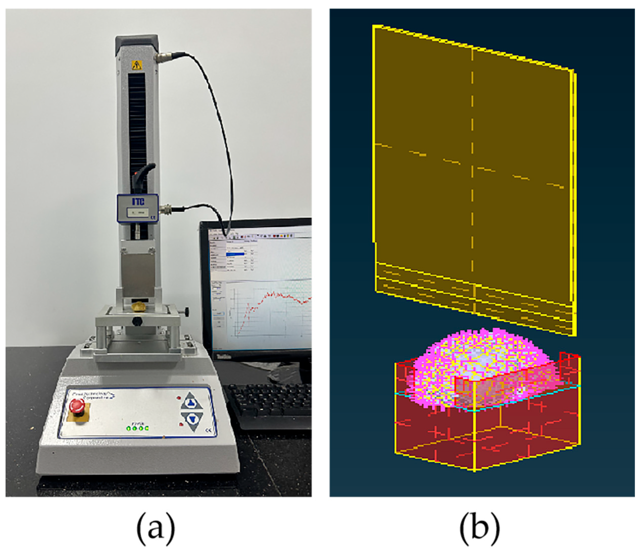
Figure 12.
Shear simulation test and actual response test of FTB. (a) Physical image of the shear verification experiment. (b) Simulation diagram of shear verification experiment.
Figure 12.
Shear simulation test and actual response test of FTB. (a) Physical image of the shear verification experiment. (b) Simulation diagram of shear verification experiment.
Figure 13.
The measured and simulated force-time curves in the uniaxial shear test.
Figure 13.
The measured and simulated force-time curves in the uniaxial shear test.
Figure 14.
Compression simulation test and response test of FTB. (a) Physical picture of compression verification experiment. (b) Simulation diagram of compression verification experiment.
Figure 14.
Compression simulation test and response test of FTB. (a) Physical picture of compression verification experiment. (b) Simulation diagram of compression verification experiment.
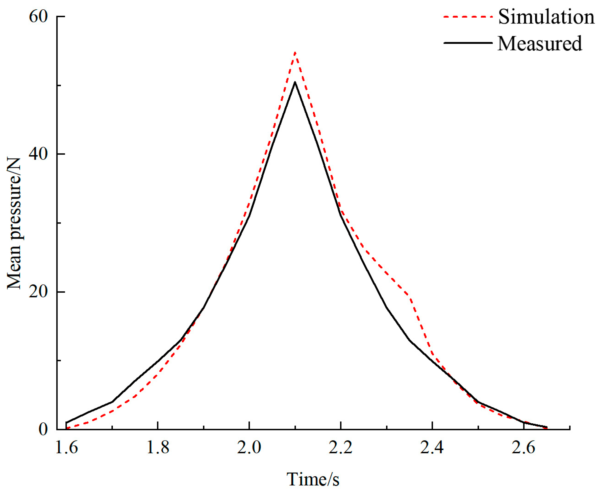
Figure 15.
The measured and simulated force-time curves in the compression test.
Figure 15.
The measured and simulated force-time curves in the compression test.
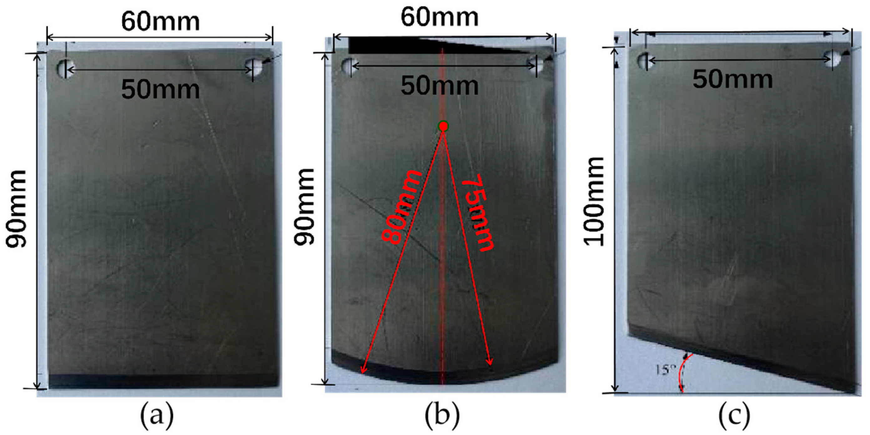
Figure 16.
Different types of blades. (a) Straight knife and its dimensions. (b) Arc knife and its dimensions. (c) Oblique knife and its dimensions.
Figure 16.
Different types of blades. (a) Straight knife and its dimensions. (b) Arc knife and its dimensions. (c) Oblique knife and its dimensions.
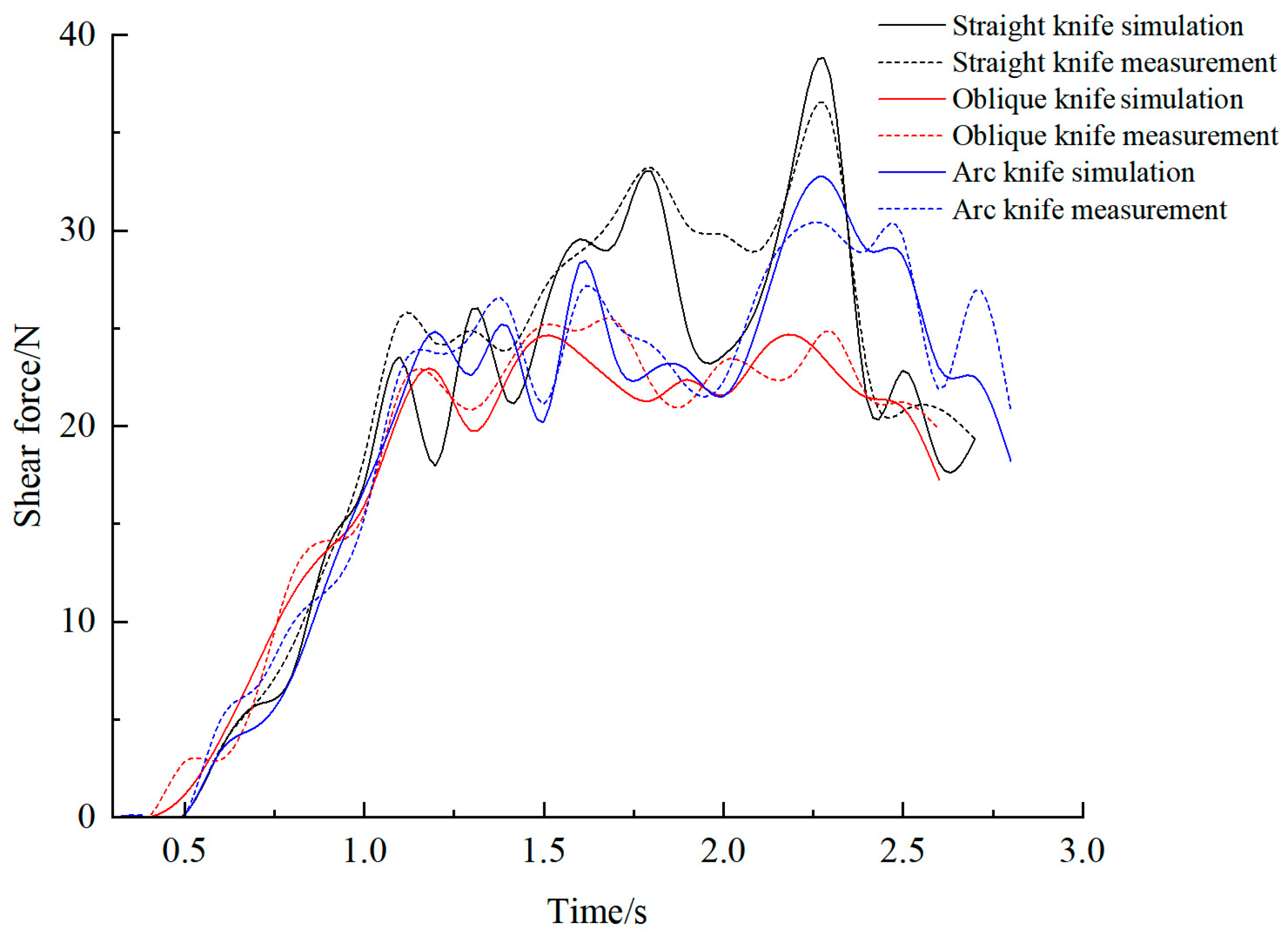
Figure 17.
The shear forces of different types of blades on FTB.
Figure 17.
The shear forces of different types of blades on FTB.
Table 1.
The intrinsic parameters of FTB.
Table 1.
The intrinsic parameters of FTB.
| Intrinsic Parameters | Values |
|---|
| Poisson’s ratio (μ) | 0.373 |
| Elastic modulus/Mpa | 7.93 |
| Static friction coefficients between FTB and the stainless steel plate f1 | 0.63 |
| Static friction coefficients between FTB and industrial rubber f2 | 0.66 |
| Coefficient of rolling friction for the interaction between FTB and the stainless steel plate μf | 0.14 |
| Coefficient of restitution between FTB and the stainless steel plate e1 | 0.606 |
| Coefficient of restitution between FTB themselves, e2 | 0.366 |
Table 2.
Simulation parameters of discrete elements of FTB.
Table 2.
Simulation parameters of discrete elements of FTB.
| Parameters | Values |
|---|
| Particle contact radius x1/mm | 1.2~2.0 |
| Normal stiffness per unit area x2/(N·m−3) | 1.0 × 10⁷~9.0 × 10⁸ |
| Tangential stiffness per unit area x3/(N·m−3) | 1.0 × 10⁷~9.0 × 10⁸ |
| Critical normal stress x4/Pa | 1.0 × 10⁶~90.0 × 10⁶ |
| Critical tangential stress x5/Pa | 1.0 × 10⁶~90.0 × 10⁶ |
| Bonding radius x6/mm | 1.2~2.0 |
Table 3.
Levels of single-factor tests.
Table 3.
Levels of single-factor tests.
| Levels | x1 | x2 | x3 | x4 | x5 | x6 |
|---|
| 1 | 1.2 | 1.0 × 10⁷ | 1.0 × 10⁷ | 1.0 × 10⁶ | 1.0 × 10⁶ | 1.2 |
| 2 | 1.4 | 5.0 × 10⁷ | 5.0 × 10⁷ | 5.0 × 10⁶ | 5.0 × 10⁶ | 1.4 |
| 3 | 1.6 | 1.0 × 10⁸ | 1.0 × 10⁸ | 10.0 × 10⁶ | 10.0 × 10⁶ | 1.6 |
| 4 | 1.8 | 5.0 × 10⁸ | 5.0 × 10⁸ | 50.0 × 10⁶ | 50.0 × 10⁶ | 1.8 |
| 5 | 2.0 | 9.0 × 10⁸ | 9.0 × 10⁸ | 90.0 × 10⁶ | 90.0 × 10⁶ | 2.0 |
Table 4.
Design and results of two-level factorial tests.
Table 4.
Design and results of two-level factorial tests.
| Serial Numbers | x1/mm | x2/(×108 N·m−3) | x3/(×108 N·m−3) | x4/(×106 Pa) | x5/(×106 Pa) | x6/mm | Maximum Shear Force/N |
|---|
| 1 | 1.6 | 1 | 1 | 5 | 5 | 1.4 | 43.1 |
| 2 | 1.4 | 0.5 | 1 | 5 | 5 | 1.4 | 29.4 |
| 3 | 1.4 | 1 | 0.5 | 5 | 5 | 1.4 | 29.8 |
| 4 | 1.6 | 1 | 0.5 | 10 | 10 | 1.6 | 40 |
| 5 | 1.4 | 1 | 0.5 | 10 | 10 | 1.6 | 40 |
| 6 | 1.4 | 1 | 1 | 10 | 10 | 1.6 | 64.8 |
| 7 | 1.6 | 1 | 1 | 10 | 10 | 1.6 | 64.8 |
| 8 | 1.6 | 0.5 | 0.5 | 10 | 10 | 1.6 | 27.1 |
| 9 | 1.6 | 0.5 | 0.5 | 5 | 5 | 1.4 | 22.9 |
| 10 | 1.6 | 1 | 0.5 | 5 | 5 | 1.4 | 29.8 |
| 11 | 1.6 | 0.5 | 1 | 10 | 10 | 1.6 | 37.9 |
| 12 | 1.4 | 0.5 | 0.5 | 10 | 10 | 1.6 | 27.1 |
| 13 | 1.6 | 0.5 | 1 | 5 | 5 | 1.4 | 29.4 |
| 14 | 1.4 | 1 | 1 | 5 | 5 | 1.4 | 43.1 |
| 15 | 1.4 | 0.5 | 0.5 | 5 | 5 | 1.4 | 22.9 |
| 16 | 1.4 | 0.5 | 1 | 10 | 10 | 1.6 | 37.9 |
Table 5.
Significance analysis of the two-level factorial test results.
Table 5.
Significance analysis of the two-level factorial test results.
| Source | Effects | Degrees of Freedom | Mean Square | F | p |
|---|
| Model | 169,000 | 6 | 28,141.88 | 19.49 | <0.0001 ** |
| A-x1 | 539.24 | 1 | 539.24 | 0.373 | 0.5563 |
| B-x2 | 136,000 | 1 | 136,000 | 93.9 | <0.0001 ** |
| C-x3 | 19,185.07 | 1 | 19,185.07 | 13.29 | 0.0054 ** |
| D-x4 | 3754.61 | 1 | 3754.61 | 2.6 | 0.1413 |
| E-x5 | 9.14 | 1 | 9.14 | 0.006 | 0.9383 |
| F-x6 | 9003.42 | 1 | 9003.42 | 6.23 | 0.034 * |
| Residual | 12,996.85 | 9 | 1444.09 | | |
Table 6.
Schemes and results of the steepest ascent method.
Table 6.
Schemes and results of the steepest ascent method.
| Serial Numbers | x2/(×108 N·m−3) | x3/(×108 N·m−3) | x6/mm | Shear Force/N |
|---|
| 1 | 0.3 | 0.3 | 1.3 | 14.3 |
| 2 | 1.1 | 1.1 | 1.38 | 37 |
| 3 | 1.9 | 1.9 | 1.46 | 75 |
| 4 | 2.7 | 2.7 | 1.54 | 106.8 |
| 5 | 3.5 | 3.5 | 1.62 | 132.5 |
| 6 | 4.3 | 4.3 | 1.7 | 141.2 |
Table 7.
Shear test, Box-Behnken experimental design, and results.
Table 7.
Shear test, Box-Behnken experimental design, and results.
| Serial Numbers | x2 | x3 | x6 | Maximum Shear Force/N | Relative Error E/% |
|---|
| 1 | 0.3 | 1.1 | 1.46 | 26.6 | 27.80 |
| 2 | 1.1 | 0.3 | 1.3 | 22.6 | 38.65 |
| 3 | 0.3 | 1.9 | 1.38 | 26.6 | 10.24 |
| 4 | 1.1 | 1.1 | 1.38 | 37 | 0.434 |
| 5 | 1.1 | 1.1 | 1.38 | 42.6 | 15.64 |
| 6 | 1.1 | 1.1 | 1.38 | 45.7 | 24.05 |
| 7 | 1.9 | 1.1 | 1.46 | 63.6 | 72.64 |
| 8 | 1.9 | 0.3 | 1.38 | 36.9 | 0.163 |
| 9 | 1.1 | 1.9 | 1.46 | 58.3 | 58.25 |
| 10 | 1.9 | 1.9 | 1.38 | 80.8 | 119.3 |
| 11 | 0.3 | 1.1 | 1.3 | 15.96 | 56.68 |
| 12 | 1.1 | 1.1 | 1.38 | 37.8 | 2.606 |
| 13 | 1.1 | 1.9 | 1.3 | 51.3 | 39.25 |
| 14 | 0.3 | 0.3 | 1.38 | 19.69 | 46.55 |
| 15 | 1.1 | 1.1 | 1.38 | 38.5 | 4.506 |
| 16 | 1.9 | 1.1 | 1.3 | 39.1 | 6.135 |
| 17 | 1.1 | 0.3 | 1.46 | 33 | 10.42 |
Table 8.
Analysis of response surface variance.
Table 8.
Analysis of response surface variance.
| Source | Effect | Degrees of Freedom | Mean Square | F | p |
|---|
| Model | 4339.0 | 9 | 482.11 | 30.32 | <0.0001 ** |
| A-x2 | 2163.18 | 1 | 2163.18 | 136.03 | <0.0001 ** |
| B-x3 | 1373.14 | 1 | 1373.14 | 86.35 | <0.0001 ** |
| C-x6 | 345.06 | 1 | 345.06 | 21.70 | 0.0023 ** |
| AB-x2x3 | 342.07 | 1 | 342.07 | 21.51 | 0.0024 ** |
| AC-x2x6 | 48.02 | 1 | 48.02 | 3.02 | 0.1258 |
| BC-x3x6 | 2.89 | 1 | 2.89 | 0.1817 | 0.6827 |
| A2-x22 | 19.53 | 1 | 19.53 | 1.23 | 0.3044 |
| B2-x32 | 33.75 | 1 | 33.75 | 2.12 | 0.1885 |
| C2-x62 | 14.43 | 1 | 14.43 | 0.9074 | 0.3725 |
| Residual | 111.32 | 7 | 15.90 | | |
| Lack of fit | 56.49 | 3 | 18.83 | 1.37 | 0.3714 |
| Pure error | 54.83 | 4 | 13.71 | | |
Table 9.
Shear test and simulation results of different types of blades on FTB.
Table 9.
Shear test and simulation results of different types of blades on FTB.
| Blade Types | Simulated Values/N | Measured Values/N | Relative Error/% |
|---|
| Flat blade | 37.6 | 36.84 | 2.06 |
| Arc blade | 32.5 | 31.82 | 2.14 |
| Oblique blade | 24.7 | 26.03 | 5.11 |

