Abstract
To enable autonomous driving in real-world environments that involve a diverse range of geographic variations and complex traffic regulations, it is essential to investigate Deep Reinforcement Learning (DRL) algorithms capable of policy learning in high-dimensional environments characterized by intricate state–action interactions. In particular, closed-loop experiments, which involve continuous interaction between an agent and their driving environment, serve as a critical framework for improving the practical applicability of DRL algorithms in autonomous driving systems. This study empirically analyzes the capabilities of several representative DRL algorithms—namely DDPG, SAC, TD3, PPO, TQC, and CrossQ—in handling various urban driving scenarios using the CARLA simulator within a closed-loop framework. To evaluate the adaptability of each algorithm to geographical variability and complex traffic laws, scenario-specific reward and penalty functions were carefully designed and incorporated. For a comprehensive performance assessment of the DRL algorithms, we defined several driving performance metrics, including Route Completion, Centerline Deviation Mean, Episode Reward Mean, and Success Rate, which collectively reflect the quality of the driving in terms of its completeness, stability, efficiency, and comfort. Experimental results demonstrate that TQC and SAC, both of which adopt off-policy learning and stochastic policies, achieve superior sample efficiency and learning performances. Notably, the presence of geographically variant features—such as traffic lights, intersections, and roundabouts—and their associated traffic rules within a given town pose significant challenges to driving performance, particularly in terms of Route Completion, Success Rate, and lane-keeping stability. In these challenging scenarios, the TQC algorithm achieved a Route Completion rate of 0.91, substantially outperforming the 0.23 rate observed with DDPG. This performance gap highlights the advantage of approaches like TQC and SAC, which address Q-value overestimation through statistical methods, in improving the robustness and effectiveness of autonomous driving in diverse urban environments.
Keywords:
deep reinforcement learning; TQC; CrossQ; SAC; TD3; DDPG; PPO; autonomous driving; CARLA simulator 1. Introduction
Autonomous driving technology enables vehicles to perceive their surroundings using a variety of sensors, such as cameras and LiDAR, and to navigate to a designated destination without human intervention by executing real-time control operations including steering, braking, and lane keeping. Traditional rule-based decision-making systems have exhibited limitations in adapting to novel or unpredictable scenarios. However, with the advancement of artificial intelligence techniques [1,2,3] and the accumulation of large-scale datasets [4,5,6], autonomous driving systems have demonstrated increasingly robust driving performances across diverse environments, progressing steadily toward becoming fully autonomous systems. In particular, perception-related modules, such as Bird’s Eye View (BEV) segmentation [7], lane detection [8], 3D object detection [9], depth estimation [10], and multi-task learning frameworks [11], have been significantly enhanced through recent advances in deep learning. Moreover, there has been growing interest in the integration of large language models (LLMs) and multi-modal large language models (MLLMs) [12,13], which aim to enrich scene understanding and enable high-level reasoning in autonomous systems [14,15]. Despite the remarkable progress in perception technologies, achieving full autonomy still necessitates moving beyond rule-based strategies in the decision-making domain. It requires adaptive and flexible learning mechanisms grounded in artificial intelligence to cope with the complexity and uncertainty of real-world driving environments [16,17,18].
To address the challenges of decision-making in autonomous driving systems, recent research has increasingly focused on using various reinforcement learning techniques. In particular, imitation learning (IL) and Deep Reinforcement Learning (DRL) have emerged as core paradigms for learning decision policies [16,17,18,19,20,21]. IL refers to the approach of learning a driving policy directly from human-expert demonstrations. While IL enables the rapid acquisition of a competent initial performance, it has been widely adopted due to its simplicity—as it often bypasses technically demanding components such as explicit reward function design and stabilization mechanisms during policy training. However, collecting comprehensive driving data for all possible scenarios from human experts is practically infeasible. As a result, IL-based approaches often suffer from generalization and scalability limitations due to issues such as covariate shift [22], error compounding [23], distributional drift [24], and recovery failure [25,26,27]. In contrast, DRL offers a more flexible learning framework, where agents autonomously learn policies by interacting with the environment and maximizing cumulative rewards. This approach eliminates the need for explicitly labeled expert data and allows the agent to learn from diverse scenarios in both simulation and real-world settings, thus addressing several key limitations of imitation-based learning. DRL therefore represents a promising direction for advancing the decision-making capabilities of autonomous driving systems.
Efforts to integrate DRL into autonomous driving have evolved in parallel with the emergence and advancement of DRL techniques. In its early stages, research was primarily driven by the success of AlphaGo, which brought significant attention to value-based methods, and particularly Deep Q-Networks (DQNs) [28]. However, since a DQN is inherently designed for discrete action spaces, its applicability in real-world driving scenarios, which typically involve continuous control, was limited. This led to the development of DRL algorithms capable of operating in continuous action spaces. Notably, several attempts were made to adapt policy-optimization-based algorithms, such as Asynchronous Advantage Actor-Critic (A3C) [29], Proximal Policy Optimization (PPO) [30], and Trust Region Policy Optimization (TRPO) [31], to autonomous driving domains. Building upon these advances, actor–critic architectures that facilitate more stable policy learning were introduced. These include the Deep Deterministic Policy Gradient (DDPG) [32], Twin Delayed DDPG (TD3) [33], and Soft Actor-Critic (SAC) [34] algorithms, which have since been widely applied in autonomous driving research. More recently, algorithms that further mitigate the problem of Q-value overestimation have been proposed, including CrossQ [35] and Truncated Quantile Critics (TQC) [36], which represent the latest advancements in DRL suitable for high-dimensional continuous control environments such as autonomous driving.
Despite the notable advancements and stabilization of DRL algorithms, several challenges remain in directly deploying these methods in real-world autonomous driving systems. Due to the inherently trial-and-error nature of reinforcement learning, training agents in real vehicles raises critical safety concerns. Moreover, collecting large-scale datasets of diverse driving scenarios requires substantial time and costs, posing a major obstacle to their practical deployment. To overcome these limitations, numerous studies have explored a progressive deployment strategy wherein the initial performance of decision-making algorithms is validated in simulation-based closed-loop environments such as CARLA (Car Learning to Act), followed by fine-tuning in real-world scenarios [37]. This approach provides a critical technical foundation for enabling real-time decision-making in diverse geographical environments—such as intersections, roundabouts, pedestrian crossings, highways, and tunnels—while adhering to traffic regulations including traffic lights, stop signs, and speed limits. In particular, the CARLA simulation environment offers a rich suite of maps representative of urban driving, an extensive collection of supporting libraries, customizable vehicles, and sensor deployment capabilities. Most notably, it benefits from a well-developed technological ecosystem that facilitates comprehensive experimentation for autonomous driving research. The ability to effectively simulate diverse driving scenarios and systematically compare the performance of autonomous agents in simulations is an essential step toward ensuring the practicality and safety of DRL-based systems in real-world deployments [38]. In line with this need, recent research has undertaken comparative and analytical evaluations of DRL algorithms for autonomous driving within simulation environments [17,38].
However, existing studies have not sufficiently incorporated a wide range of state-of-the-art DRL algorithms into these assessments, and many lack realistic urban environmental elements such as traffic lights and road infrastructure. In particular, prior research often applies DRL algorithms in isolation, without conducting a comprehensive comparative analysis under unified evaluation criteria. For example, the study in [38] compares DQN and DDPG using the CARLA simulator, ref. [39] evaluates DQN and PPO, and [40] focuses solely on a comparison between DQN and DDPG. These fragmented efforts limit the generalizability and depth of our insight into the relative performance of modern DRL algorithms for autonomous driving. To address this gap, the present study applies six representative DRL algorithms—DDPG [32], PPO [30], SAC [34], TD3 [33], CrossQ [35], and TQC [36]—to urban autonomous driving scenarios in the CARLA simulator [41]. These scenarios include complex geographic environments such as intersections, roundabouts, crosswalks, highways, and tunnels, while incorporating real-world traffic rules including traffic lights, stop signs, and speed limit compliance. This study presents an in-depth evaluation of each algorithm’s driving performance, the effectiveness of its associated reward functions, and a comparative analysis of their Success Rates across diverse urban driving conditions.
2. Related Works
This section reviews prior research efforts that have used DRL for autonomous driving, focusing on the methodologies employed and their associated limitations. We first examine foundational studies aimed at developing efficient DRL-based autonomous driving systems and follow this with comparative evaluations of various DRL algorithms.
Early approaches to decision-making in autonomous driving primarily relied on IL, where an agent learns to mimic the behavior of a human expert [25,26,42,43,44,45,46,47].
One of the earliest attempts to apply IL to autonomous driving is presented in [42], where a neural network was trained via supervised learning to predict steering angles from a camera input. This study was also among the first to experimentally highlight the problem of covariate shift in IL-based driving.
In [43], the authors proposed PilotNet, a pioneering end-to-end driving model that extracted visual features from camera images using a convolutional neural network (CNN) and directly output steering commands. The model was trained using behavior cloning on a large-scale human driving dataset. However, its trajectory completion performance was limited in complex scenarios. To enhance IL, ref. [25] introduced a hierarchical command-conditioned imitation learning approach, where high-level navigational commands (e.g., turn left/right, go straight) guided the agent’s behavior. In [26], the authors proposed Generative Adversarial Imitation Learning (GAIL), in which a discriminator network distinguishes between expert and learner trajectories, thereby guiding the agent to produce expert-like behavior through adversarial training. Similarly, ref. [44] presented a generative model that learns trajectory distributions via Conditional Variational Autoencoders (VAEs), enabling multi-modal trajectory generation through flexible planning. In [45], an end-to-end learning environment was established by integrating the CARLA simulator with OpenAI Gym, where deep imitation learning was empirically validated through autonomous driving experiments. However, these IL-based approaches had significant limitations in their generalization and scalability due to common issues such as covariate shift [22], error compounding [23], distributional drift [24], and recovery failure [25,26]. To mitigate such limitations, hybrid approaches combining IL and reinforcement learning have been explored. For example, ref. [46] proposed a Hierarchical Behavior and Motion Planning (HBMP) framework, integrating PPO with DAGGER-based imitation learning to enable efficient and safe lane-change planning. Likewise, ref. [47] attempted to overcome the limitations of IL by combining it with SAC, leveraging the strengths of both paradigms. Nevertheless, these hybrid approaches represent transitional efforts made during a period when DRL techniques had not yet fully matured. As DRL methodologies have advanced, the focus of research has increasingly shifted toward direct policy learning through DRL itself, aiming to exploit its full potential in autonomous decision-making tasks.
Early research on autonomous driving decision-making using DRL predominantly focused on the Deep Q-Network (DQN) algorithm [28] and its variants, such as Double DQN (DDQN), Dueling DQN (DulDQN), and Prioritized Experience Replay DQN (PRDQN) [39,40,48,49,50,51,52,53]. While these methods laid foundational groundwork for learning decision policies, their applicability in real-world driving was limited by the discrete nature of the action space inherent to a DQN, making it difficult for it to directly learn fine-grained control signals such as steering angles and throttle commands.
To address this limitation, several DRL algorithms were subsequently proposed to handle continuous action spaces, including those based on deterministic actor–critic architectures. Among these, the Deep Deterministic Policy Gradient (DDPG) algorithm [32] gained significant attention, leading to its application in various autonomous driving studies [37,54,55,56,57,58,59]. In [54], the authors introduced Controllable Imitative Reinforcement Learning (CIRL), a vision-based end-to-end control framework for urban driving. CIRL combines model-based supervised learning with DDPG in a dual-stage training procedure to overcome the exploration inefficiency of RL and the generalization limitations of imitation learning. Ref. [57] proposed a hybrid framework that combines affordance learning and DDPG for urban autonomous driving. In this approach, a high-dimensional camera input is processed by a CNN to extract six key environmental factors: (1) steering angle deviation, (2) traffic light state (e.g., red light detection), (3) distance to the leading vehicle, (4) speed limit, (5) lateral lane offset, and (6) presence of hazards (e.g., pedestrians). These affordances, along with vehicle speed and lane departure information, are used to generate continuous control outputs for steering, acceleration, and braking. Ref. [37] proposed a two-stage DDPG framework for the car-following problem in autonomous vehicles, combining both real-world and simulated data. In the first stage, the agent is trained in the CARLA simulator using standard DDPG. In the second stage, additional fine-tuning is performed using real driving data from the Napoli dataset via a practical replay buffer, enhancing the policy’s adaptability to real-world dynamics. While DDPG is effective for continuous control, it is based on a deterministic actor–critic structure, which makes it vulnerable to Q-value overestimation. This leads to performance degradation in situations involving multi-modal decision-making, which are commonly encountered in complex autonomous driving tasks.
In response to the limitations of deterministic actor–critic methods, a new line of research has emerged that seeks to mitigate the Q-value overestimation problem through stochastic policy-based approaches. Among these, PPO [30], which constrains policy updates via a clipping mechanism, has been applied to various autonomous driving decision-making tasks [60,61,62,63]. In [60], the authors proposed an end-to-end autonomous driving policy learning method that integrates PPO with curriculum learning in the CARLA simulator. The study demonstrated that even without prior knowledge, the agent could learn robust driving behaviors through a staged curriculum with gradually increasing task difficulties. Additionally, the authors addressed issues related to unstable value function updates and the normalization of the advantage function. Ref. [61] applied PPO to the tactical decision-making problem for autonomous vehicles navigating intersection scenarios, with the goal of ensuring both safety and efficiency during maneuvering. In [63], the authors conducted a comparative study of DDPG and PPO in the TORCS simulator, evaluating their performance in lane-keeping, obstacle detection, and collision avoidance tasks. While PPO has shown promise in improving stability and reducing Q-value overestimation to some extent, it is fundamentally an on-policy algorithm. As such, it requires repeated rollouts with fresh data, making it sample-inefficient compared to its off-policy counterparts. Furthermore, its limited capacity to fully resolve overestimation issues has led to performance bottlenecks in complex autonomous driving scenarios.
To overcome the performance limitations of DDPG and PPO, TD3 [33] was introduced as an enhancement to DDPG, specifically designed to address the Q-value overestimation problem. TD3 improves policy learning stability by employing a double critic architecture and selecting the minimum of the two Q-value estimates. Furthermore, it introduces policy smoothing by adding clipped noise to the target policy values, which mitigates overfitting to narrow Q-function peaks. As an off-policy method, TD3 also improves sample efficiency, making it suitable for continuous control in complex driving environments [64,65,66,67]. In [64], TD3 was applied to a human–machine shared driving framework for lane-changing decision-making. The study demonstrated that TD3’s capability for fine-grained continuous control allowed for more natural and safe lane transitions in mixed traffic scenarios. Further studies [65,66,67] explored the use of TD3 in high-density urban intersections, aiming to enhance both its safety and driving efficiency. Notably, ref. [67] proposed a hybrid TD3+Behavior Cloning (TD3+BC) algorithm, which achieved up to a 17.38% improvement in intersection navigation efficiency, demonstrating the potential of combining reinforcement learning with expert-driven priors. Despite its advantages, TD3 remains a deterministic policy algorithm, which limits its ability to represent multi-modal action distributions. This constraint may reduce the agent’s adaptability in situations where multiple plausible actions exist, thereby restricting its responsiveness to highly dynamic and uncertain environments.
The SAC algorithm [34] was proposed as an enhancement of TD3, aiming to address the limitations of deterministic policies in dynamic environments by introducing the concept of the soft Q-function. Unlike traditional Q-functions, which solely accumulate rewards, the soft Q-function incorporates both the expected cumulative reward and the entropy of the current policy, thereby encouraging policy stochasticity and enhancing exploratory behavior during learning [68,69,70,71,72]. In [68], the authors proposed a hybrid method that combines the SAC-Discrete algorithm with a motion-prediction-based safety controller to address the highway merging problem in mixed traffic environments. Their approach demonstrated significant improvements in reducing collision rates and increasing traffic flow efficiency across varying traffic densities in simulations. Ref. [69] employed the SAC algorithm to manage the roundabout entry problem in complex urban scenarios. Their method leveraged a CNN-based feature extractor combined with a destination vector to enable smooth and safe vehicle navigation through roundabouts. Experimental results using the CARLA simulator indicated that the SAC-based policy achieved faster convergence and higher Success Rates compared to DQN and PPO. In [70], the SAC framework was integrated with a residual sensor fusion approach that combines image sensor and tracking sensor data for enhanced control policy learning. This technique improved the learning performance of the autonomous agent by leveraging complementary sensor modalities, yielding robust results across multiple autonomous driving scenarios.
While TD3 and SAC have demonstrated the ability to mitigate Q-value overestimation, residual overestimations—particularly in nonlinear critic networks—continue to be a source of instability in policy learning. To address this, CrossQ [35] introduces a novel approach based on cross-critic regularization, which incorporates an additional regularization term that enforces mutual alignment between two critic networks. This regularization discourages the critics from diverging excessively during training, thereby improving the stability of value estimates. Despite its conceptual promise, CrossQ is a relatively recent development, and no prior studies have explored its application within the autonomous driving domain. To the best of our knowledge, this work is the first to apply CrossQ in urban autonomous driving scenarios and to conduct a comparative analysis with other state-of-the-art DRL algorithms under realistic driving conditions.
Lastly, TQC [36] was proposed to address the instability in policy updates caused by noisy Q-values in the upper quantiles of the estimated value distribution. TQC builds on the principles of distributional reinforcement learning, where the critic learns a full distribution of Q-values rather than a single scalar estimate. By truncating the highest quantiles, which are often noisy and overestimated, TQC constructs a more robust Q-target, improving both its learning stability and representational accuracy. Although TQC offers a theoretically grounded approach to reducing Q-value overestimation while capturing uncertainty in future rewards, it remains underexplored in the field of autonomous driving. As such, this study represents the first empirical investigation of TQC’s performance within autonomous driving tasks, providing a comparative evaluation against other leading DRL techniques.
Table 1 summarizes the studies related to the application of DRL in the field of autonomous driving, as discussed above.

Table 1.
Summary of DRL approaches in autonomous driving.
Accordingly, this study establishes a comprehensive DRL-based autonomous driving framework within the CARLA simulator, incorporating diverse geographic environments—including intersections, roundabouts, crosswalks, highways, and tunnels—as well as various traffic regulations such as traffic lights, stop signs, and speed limits.
The primary contributions of this study are summarized as follows:
- This work presents the first application of CrossQ and TQC in autonomous driving, conducting a comprehensive comparative analysis of their performance alongside that of existing algorithms such as DDPG, PPO, SAC, and TD3. Evaluations are performed within a closed-loop simulation environment that incorporates diverse geographic variations and complex traffic regulations. The analysis also includes a detailed investigation of failure factors, from which key insights for algorithmic improvements are derived.
- A set of comprehensive evaluation metrics is proposed to assess driving performance under varying geographic and regulatory conditions. These metrics capture multiple dimensions of performance, including the effectiveness, stability, efficiency, and comfort of driving.
- A set of adaptive reward and penalty functions is designed to facilitate effective policy training under dynamic driving scenarios that reflect complex geographic variations and real-world traffic regulations, enhancing the robustness and generalization of DRL-based decision-making.
3. System Model
3.1. Policy Network Model
Figure 1 presents a schematic overview of how the system operates, including the CARLA simulator and the interacting DRL module. Among the core tasks of autonomous driving, i.e., perception, decision-making, and control, the CARLA simulator is responsible for perception by collecting the camera-based visual information required for downstream decision-making. This perceived information is then transmitted to the DRL module, which performs decision-making based on a reinforcement learning algorithm. The resulting control actions are subsequently processed through action smoothing (a weighted sum between the previous and current action values) and sent back to the CARLA simulator to control the ego vehicle. Finally, the resulting reward for the executed action is fed back to the DRL module to evaluate the action and update the policy accordingly.
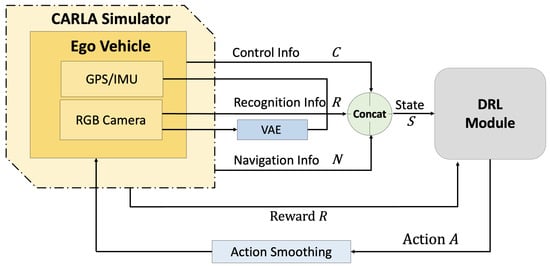
Figure 1.
Brief system operation of CARLA simulator and DRL module.
In detail, the CARLA simulator receives front-facing RGB images from the ego vehicle and processes them using the Variational Autoencoder (VAE) network illustrated in Figure 2, producing segmentation outputs that encode essential environmental features such as road lines, road surfaces, and sidewalks. In addition, sensor data that describe the current state of the vehicle—namely RGB camera feeds, GPS signals, and IMU measurements—are used to estimate the vehicle’s position and heading angle. These perception-related observations, denoted by , are concatenated and forwarded to the DRL module. Furthermore, the DRL module receives navigation-related information from the CARLA simulator, which includes the coordinates of the next 15 waypoints and the state of traffic lights within an approximate 18 m forward range. Here, the 15 forward waypoint coordinates are initially determined by Global Path Planning (GPP) using the algorithm [73,74]. The 15 waypoints are selected based on their proximity to the vehicle’s current position, while also considering road curvature, lane geometry, and junction structures. Lastly, the DRL module is also provided with the current control information of the vehicle , including its steering angle , throttle , brake , and velocity . The output range of each control parameter is defined as follows:
where is defined as a normalized value ranging from to , corresponding to a steering angle between and . When considering a conventional vehicle operating below 9000 Revolutions Per Minute (RPM), the throttle value is mapped to a propulsion torque of Nm. Similarly, the brake value is mapped to a braking torque of Nm. It is important to note that when the brake value is activated, the throttle is automatically set to zero, and vice versa, ensuring mutual exclusivity between the throttle and braking operations.
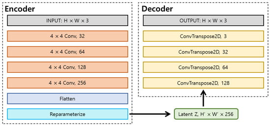
Figure 2.
VAE architecture: the image features are extracted through four convolutional layers to generate the latent space Z, which is subsequently decoded into a segmentation image using four transposed convolutional layers.
This information is integrated into the vehicle state information and provided to the DRL module. The DRL module then utilizes the vehicle state information to compute an optimal control action, which is passed through an action smoothing process to mitigate abrupt behavior changes before being applied to the environment. Subsequently, the next state and corresponding reward are received as feedback. This interaction constitutes a single step, and the system operates at a frequency of 15 steps per second (SPS), where each step corresponds to approximately 66.7 ms. At each step, a driving decision is made and an associated reward is assigned accordingly.
Figure 3 illustrates the temporal structure of the experiment. Each experiment is conducted in episode-based units, where a predefined driving route is assigned per episode, and each episode comprises a sequence of multiple steps. If the ego vehicle violates a traffic regulation, a penalty, represented as a negative reward, is imposed, and the episode is immediately terminated. The details of the reward function and its components are discussed further in Section 3.4.
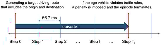
Figure 3.
A conceptual illustration of the approximate timing and granularity of the simulation operation.
3.2. DRL Module
The key parameters that constitute the DRL module are defined as follows: the ego vehicle serves as the agent that performs actions, while the environment represents the external world with which the agent interacts. The environment is modeled as a state , which can be represented at each time step t as . The state space is identical to the vehicle state information provided by the CARLA simulator. The action is defined as , where the action space is composed of all elements of the control information C except for : . The reward is defined as .
Policies are categorized into two types depending on whether their probability distributions are deterministic or stochastic. In the case of a deterministic policy, the selection of action a given state s is defined as . In contrast, for a stochastic policy, the probability distribution of actions a given state s is denoted as . The transition probability from a state s to a subsequent state under action a is represented as . The discount factor for future returns is denoted by . At each time step t, the return is represented by , the corresponding state value function under policy is denoted as , and the action value function is given by , which are formally defined as follows:
Table 2 summarizes the key characteristics of the DRL modules utilized in the experiments, while Figure 4 provides a schematic comparison of the architectural structures of each algorithm.
Table 2.
Characteristics of DRL algorithms.

Figure 4.
A comparative overview of the DRL algorithms used in the experiment and their corresponding module architectures.
DDPG follows a standard actor–critic framework, employing target networks for both the actor and critic to stabilize Q-value estimation and policy learning.
Let us now provide a formal mathematical formulation. The current reward is combined with the output of the target critic evaluated in the next state and the action selected by the target actor (policy) , resulting in the target Q-value being the learning objective. The target network is introduced to mitigate the instability caused by abrupt parameter updates. Accordingly, the target Q-value can be expressed as follows:
The Q-network is subsequently trained using the mean squared error (MSE) loss to minimize the discrepancy between the current estimate and the previously defined target value , as expressed by the following objective:
Finally, for policy optimization, the gradient of the deterministic policy is updated indirectly via the Q-network by applying the chain rule, as formulated below:
In contrast, TD3 improves upon DDPG by introducing two critic networks and employing a minimum Q-value selection strategy for the target critics to mitigate overestimation within the critic module.
Then, the target Q-function , which selects the minimum value between the two Q-networks and , can be expressed as follows:
where the exploration noise is introduced to prevent overfitting and is defined using a value sampled from and clipped within the range .
The loss function for the Q-update can be defined as follows:
where and denote the neural network weights of the two Q-networks, and , respectively.
Each policy is updated periodically, and for the sake of stability, the update is performed based solely on :
SAC utilizes a stochastic policy and performs critic updates based on the smaller of the two Q-values from the critic and target critic, while also incorporating an entropy bonus into both policy and critic updates to encourage exploration.
Therefore, the target Q-network in SAC can be formulated as follows by incorporating the entropy bonus:
where denotes the entropy temperature coefficient, which regulates the contribution of the entropy term.
Similarly, to ensure that the predicted Q-value for the current state–action pair closely approximates the target , the critic network is optimized using the loss function , which is formulated as follows:
Through this formulation, the policy is updated to favor actions with higher estimated returns—based on the minimum of the two Q-values—while simultaneously promoting diversity by incorporating an entropy term.
TQC is an algorithm that extends SAC within the distributional reinforcement learning paradigm. It leverages an ensemble of critic networks to estimate quantile-based return distributions and applies a truncation-and-averaging mechanism to both the critic and target critic by discarding excessively high quantile values and averaging the remaining ones. This approach is motivated by the tendency of upper quantiles to induce overestimation, and thus TQC has improved policy stability.
The target value for Q-learning can be formulated as follows:
where denotes the quantile-based Q-values, representing the predicted return values for a given state–action pair, as a set of K quantiles. In other words, among the total K quantiles, the top M quantiles prone to overestimation are discarded, and the remaining lower quantiles are retained. The mean of these retained quantiles is then used to compute the target Q-value.
Furthermore, the loss function for the Q-update is formulated as follows:
where represents the Quantile Huber Loss, N is the number of critic networks, and denotes the j-th quantile output of the i-th critic network evaluated in the state–action pair .
The policy update follows the same principle as that in SAC, incorporating the entropy term along with multiple Q-networks. The update is performed using the mean of the truncated quantile Q-values as follows:
CrossQ extends the conventional DDPG and TD3 architectures by introducing a conservative Q-update scheme based on a cross-validation mechanism. Specifically, it constructs multiple actor–critic pairs, where each actor–critic pair participates in target generation and value estimation for the others in a crosswise manner. This design mitigates the overestimation bias by avoiding self-referential updates, thus promoting more conservative and stable learning dynamics. Furthermore, to enhance training stability, CrossQ integrates batch renormalization into the critic architecture.
This can be formulated as follows:
where denotes the action generated by the i-th actor for the next state and represents the predicted Q-value from the j-th critic corresponding to that action.
In Equation (16), the condition implies that the action used to compute the target Q-value is generated by actor i’s policy, while the corresponding Q-value is evaluated using critic j. By selecting the minimum of multiple Q-values, the approach enables a more conservative Q estimation. This cross-validation mechanism prevents an actor from evaluating the Q-value of its own generated actions using its corresponding critic, thereby mitigating overfitting and overly optimistic value estimates.
The loss function for the Q-update is defined as follows:
Additionally, for the policy update, the action is generated based on the policy of actor i, and the update is performed using the evaluation from the critic :
PPO is an on-policy reinforcement learning algorithm that seeks to balance sample efficiency and training stability. It leverages trajectory memory to estimate advantage values and computes the probability ratio between its current and previous policies. A clipped surrogate loss function is then formulated and minimized to update the policy, while constraining large updates to ensure stable learning. Unlike previous off-policy algorithms that rely on a state–action value function for their critic, PPO employs the state value function to perform the critic’s role.
The clipped surrogate loss function used to update the policy network is defined as shown below. It compares the probability of actions under the new policy and the old policy using an importance sampling ratio.
where denotes the advantage estimate at time step t, and is a small hyperparameter (typically in the range of 0.1–0.2) introduced to limit the extent of policy updates. Additionally, the importance ratio is defined as follows:
where the probability ratio is between the new policy and the old policy for the action actually taken at state . It acts as a correction factor in the surrogate objective.
Finally, the regression loss function based on the value function is defined as follows:
where is a target value computed from the returns.
3.3. VAE Encoder
To enhance the stability and efficiency of policy learning in complex urban environments, we adopt a VAE-based encoder for the visual perception component of the agent’s state vector. In contrast to conventional CNN-based encoders, which tend to produce high-dimensional and semantically opaque latent representations, the VAE compresses high-resolution visual data into a structured low-dimensional latent space. Each latent variable is trained to follow a standard Gaussian distribution, enabling the representation to retain semantically meaningful features such as lane count and object density. This not only facilitates better interpretability of the latent space but also acts as a form of regularization by enforcing smoothness and disentanglement across the latent dimensions. Prior studies [75,76] have empirically demonstrated that under the same reinforcement learning algorithm, agents utilizing VAE-based encoders outperform their CNN counterparts in terms of average rewards and driving distance, while also reducing GPU usage and improving inference speed. These findings provide strong evidence that the VAE serves as an effective representation learner, offering superior capacity, regularization benefits, and interpretability compared to alternative encoder architectures.
3.4. Reward Function
The reward function for the agent is primarily designed to encourage speed maintenance, lane keeping, and traffic rule compliance. The detailed structure of the reward functions used is summarized in Table 3.
Table 3.
Reward and penalty parameters comprising the total reward function.
3.4.1. Reward
The underlying philosophy of the reward’s design is centered on promoting safe and compliant driving behavior. To this end, the reward function contains multiple contributing factors that encourage the agent to (1) maintain an appropriate speed, (2) stay within lane boundaries, (3) align its heading with the road direction, and (4) obey various traffic regulations. These objectives are jointly enforced through a composite reward function.
Throughout each episode, driving decisions are made at every decision step, and a reward value ranging from 0 to 1 is assigned at each step. The cumulative reward accumulated over the course of an episode is employed as a quantitative measure of overall driving performance. The individual reward components and their corresponding formulations, computed at each step, are presented as described below.
The Speed Reward is computed based on the current traffic signal state. Specifically, it is categorized as follows: for a green light, indicating normal driving conditions; for a red light, requiring the vehicle to stop; and for a yellow light, suggesting deceleration.
When a green light is active or the vehicle is navigating a section with no available traffic light information, the speed reward assigned is , which can be calculated according to Equation (22):
where denotes the current speed of the ego vehicle. The reward value is designed to yield higher scores when lies within the desirable range, between the minimum speed threshold and the target speed . If falls below or exceeds , the reward is gradually reduced. Furthermore, if the vehicle exceeds the maximum allowable speed , a negative reward is applied to penalize unsafe driving. In the experimental setup of this study, the parameters used were as follows: = 25 km/h, = 20 km/h and = 35 km/h.
In the case of a red traffic light, the Speed Reward value is formulated as in Equation (23), such that the vehicle is encouraged to approach the stop line gradually from its current position.
where and denote the weighting coefficients for the distance to the stop line and the ego vehicle’s speed, respectively. In the experiment, they were set to 0.4 and 0.6. The terms and represent the normalized values of the distance from the vehicle’s current position to the stop line and the current speed of the ego vehicle , respectively. The corresponding normalization formulas are defined in Equations (24) and (25).
where denotes the maximum allowable distance from the current vehicle position to the stop line, which was set to 30 m in this experiment. In other situations, specifically, when the traffic light is yellow, the vehicle is designed to drive defensively at a minimum speed . To implement this behavior, the Speed Reward is defined according to Equation (26):
To encourage the vehicle to maintain lane alignment during driving, the reward function is designed to assign higher rewards when the vehicle remains close to the center of the road. Accordingly, the Centerline Distance Reward is defined as in Equation (27):
where denotes the Euclidean distance between the current position of the vehicle and the center of the road. represents the maximum allowable value of , which was set to 3 m.
To further promote stable driving along the road centerline, the Centerline Standard Deviation Reward, based on the standard deviation of the centerline distance, , is defined as shown in Equation (28):
where denotes the standard deviation of the distance between the ego vehicle and the road centerline during driving. represents the maximum allowable standard deviation, which was set to 0.4 in this experiment.
The Vehicle Heading Reward is designed to prevent abnormal directional deviations, such that higher rewards are given when the vehicle’s heading aligns closely with the road direction. This reward is defined by Equation (29):
where represents the heading angle between the vehicle’s current orientation and the road direction, while denotes the maximum allowable heading angle, which was set to in this experiment.
3.4.2. Penalty
The refers to the negative reward of −10 that is assigned when an episode terminates due to abnormal driving conditions. This penalty is applied upon the occurrence of events such as vehicle stopped, off-track, too fast, red light violation, and collision.
where refers to the case in which the vehicle’s speed remains below 1.0 for more than 10 s without a stop signal, occurs when the vehicle deviates beyond the allowable maximum distance from the road centerline, corresponds to situations where the vehicle exceeds the predefined maximum allowable speed , is triggered when the vehicle passes through an intersection despite a red traffic light signal, and finally occurs when the vehicle collides with an obstacle.
3.4.3. Total Reward Function
Based on the previously defined reward values and penalty values, the Total Reward Function in each step is computed as shown in Equation (31). Here, P is a parameter representing the penalty value, which remains zero under normal driving conditions in which no penalty violations occur.
4. Evaluation Metrics
This section introduces the evaluation metrics used to assess the performance of DRL-based autonomous driving techniques. These metrics are defined for a given driving episode i in terms of the travel distance, Route Completion, driving stability, and cumulative reward.
- Travel Distance : The distance traveled by the agent during episode i is calculated by cumulatively summing the distance covered at each step until the final time step, as illustrated in Figure 3.
- Route Completion : This metric represents the proportion of the intended route , generated from the start to the destination in episode i, that the ego vehicle successfully traveled from the starting point. It is computed according to Equation (32):
- Speed Mean : This metric denotes the average speed of the ego vehicle over the entire duration of episode i and is computed as shown in Equation (33).where represents the vehicle’s speed at each step t and denotes the total number of steps in episode i.
- Centerline Deviation Mean : This metric quantifies how far the vehicle deviates from the lane centerline during driving and is computed according to Equation (34). It is based on the average of the Centerline Deviation values at each time step. A smaller value indicates stable lane keeping, whereas a larger value suggests a higher likelihood of lane departure.
- Episode Reward : Episode Reward represents the total cumulative reward obtained by the agent during episode i and is computed according to Equation (35).
- Episode Reward Mean and Step Reward Mean : The average reward metric is defined along two temporal scales. The first is the Episode Reward Mean, which is calculated by summing the total rewards obtained across all N episodes and dividing by the number of episodes. This metric represents the average reward per episode and is computed according to Equation (36). The second is the Step Reward Mean, which is calculated by dividing the total episode reward by the total number of steps in episode i. This metric represents the average reward per step and is computed according to Equation (37).
- Reward Standard Deviation : This metric represents the variability of the rewards obtained by the agent during episode i and is defined as shown in Equation (38). A lower value indicates that the learned policy is more stable and consistently acquires rewards.
- Success Rate : For each episode i, the binary success indicator is defined according to Equation (39), which determines whether the ego vehicle successfully reached its destination. In this formulation, an episode is considered successful () if the final vehicle position is within 5 m of the goal position . Otherwise, it is considered a failure (). The overall Success Rate is then computed by averaging the success indicators across all N episodes, as defined in Equation (40).where N denotes the total number of executed episodes.
5. Experimental Setup
5.1. CARLA Simulation Map
The simulation environment used in the experiments was based on five urban maps provided by CARLA. Figure 5 illustrates the layout of each town map, while Table 4 summarizes the specific driving environment characteristics of each town. Table 5 presents the durations of the traffic light cycles for each town. As shown in Figure 5, a total of five towns were selected, with four distinct driving episodes assigned to each town. The route length of each episode ranged from a minimum of 150 m to a maximum of 900 m.
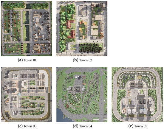
Figure 5.
CARLA town maps used in the experiments.
Table 4.
Driving environment variations across five urban towns.
Table 5.
Traffic light cycle durations in each CARLA town (s).
In this study, we used all five towns presented in Figure 5, which are publicly available and designed for urban driving scenarios, from the ten towns provided in CARLA version 0.9.13.
Town02 features the smallest map among the five towns, characterized by a relatively simple road layout with a limited number of T-shaped intersections and traffic lights. Despite its compact size, it contains a large number of signalized intersections, making it particularly suitable for the initial policy learning of reinforcement learning agents being trained under diverse traffic regulations and geographical variations. In contrast, Town01 is a small urban map that also includes numerous T-intersections and traffic signals, offering a similar baseline environment for early autonomous driving experiments.
Town03 includes a small number of cross-shaped intersections and two-lane roads. It is the only town among the five that contains a roundabout and a tunnel, thus providing a more complex setting in which to evaluate the models’ driving performance under diverse geographic variations. Town04 features the widest roadways, with four-lane highways, and includes a highway driving scenario. It is used to train and evaluate mixed urban and highway driving strategies, including highway merging, exiting, and lane changes. Town05 incorporates the greatest number of cross-shaped intersections and traffic lights, along with highway and multi-lane roads. It is designed to challenge agents with high-level intersection handling, frequent lane changes, and responsiveness to traffic signals [77].
To evaluate the generalization capabilities of the learned driving policies, training was conducted exclusively in Town02, where the driving route was randomly set for each episode. Table 6 summarizes the maximum route lengths (in meters (m)) of each episode run across the five towns (Town01–Town05) for the training policy.
Table 6.
Driving distance per episode (m).
Town01 includes the episode with the longest driving distance, featuring a total route length of 2752 m, and has an average episode length of 688 m, which is more than twice that of the other towns. Despite its relatively simple road structure, the extended route lengths in Town01 increase its difficulty. In contrast, Town02 offers the shortest evaluation paths, with a total distance of 908 m and an average of 227 m, indicating that the agent was trained repeatedly on relatively short trajectories.
Finally, Figure 6 illustrates a representative driving scenario, presenting (a) the front-view RGB image input received by the VAE, (b) the reconstructed segmentation observation generated by the decoder, and (c) the RGB image overlaid with waypoints corresponding to the current environment. The perceptual information from (a) and (b) is integrated into the Recognition module R as described in Figure 1 and subsequently utilized within the DRL framework as part of the state representation used for training the policy network.
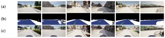
Figure 6.
Visual overview of the observation pipeline. (a) Raw front-view RGB image perceived by the vehicle. (b) VAE decoder output, with segmentation-style reconstruction. (c) Waypoint-guided RGB image captured by a front observer camera, which is not part of the agent’s input but serves as a reference.
5.2. Hyperparameter Setup for DRL Training
The critical hyperparameter configurations for the DDPG, SAC, TD3, PPO, TQC, and CrossQ algorithms are outlined below. For all algorithms, an exponential decay learning rate schedule was adopted, whereby the initial learning rate was set to and gradually decreased throughout training to . This approach enables rapid exploration during the early training phase while promoting stability and convergence in the later training stages.
For the on-policy algorithm PPO, which does not utilize a replay buffer, training was conducted using newly sampled data at every iteration. Accordingly, the number of steps collected from the environment per training iteration was set to 1024, and the number of epochs, i.e., how many times the collected data is reused for policy updates, was set to 10.
In contrast, all other algorithms (DDPG, SAC, TD3, TQC, CrossQ) are off-policy methods. These models train by sampling transitions from a replay buffer of size 300 K, which enables improved sample efficiency and policy refinement over extended training horizons.
The model complexity and inference latency of each trained DRL algorithm are summarized in Table 7. The model size (in MB) is reported separately for the actor (policy), critic, and target networks (target policy and target critic). All algorithms employ a uniform neural network architecture denoted as [400, 300], which refers to a fully connected network with two hidden layers consisting of 400 and 300 neurons, respectively, followed by an output layer. In this configuration, each individual network with the [400, 300] architecture contains approximately 0.62 MB of parameters.
Table 7.
Model size and inference latency.
Inference latency was measured in the Town02 scenario. For all algorithms, the average step-wise latency was computed over 4.5 k steps.
As shown in Table 7, despite TD3 having the largest total model size, it demonstrates relatively low inference latency. In contrast, TQC has both a moderately large model size and relatively high latency. Meanwhile, DDPG and PPO incur the lowest latency among the evaluated algorithms.
6. Simulation Result
Each algorithm was trained for 1 million steps, and performance varied according to the structural characteristics and learning paradigms of each method.
Figure 7 visualizes the progression of six performance metrics—the Episode Reward Mean, Step Reward Mean, Route Completion Rate, Success Rate, Centerline Deviation Mean, and Speed Mean—across training checkpoints from 200 k to 1 M steps. In particular, the Step Reward Mean graph represents the average reward received per step. As observed in Figure 7, there is no strict proportional relationship between the Episode Reward Mean and Step Reward Mean. This discrepancy arises because the Episode Reward denotes the total cumulative reward over an entire driving episode, while the Step Reward Mean reflects the average reward per time step. Consequently, a high Episode Reward Mean does not necessarily imply a high Step Reward Mean, particularly in longer or partially successful episodes. Therefore, the joint interpretation of both metrics enables a more precise evaluation of each algorithm’s performance in terms of both its overall driving success and per-step reward efficiency.
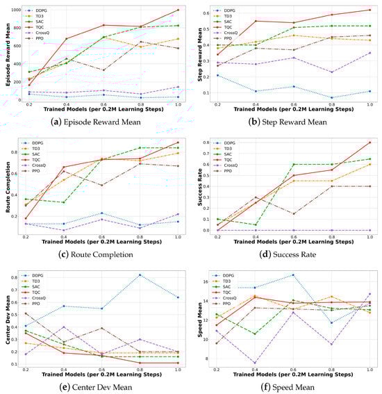
Figure 7.
Performance variation trends over 1M steps of learning.
In Section 6.1, Section 6.2 and Section 6.3, the model that achieved the best performance within the 200 K–1 M steps of learning for each algorithm is selected and compared across key evaluation metrics in tabular format. Furthermore, Section 6.4 provides a quantitative analysis of penalty occurrence rates, as defined in Section 3.4, for each algorithm and town. To ensure the statistical reliability of the penalty evaluation, five additional trials were conducted per route scenario. The average penalty ratio was then computed based on the aggregated results.
TQC exhibited the most outstanding performance across all evaluation metrics, achieving top values in Episode Reward Mean, Step Reward Mean, Route Completion, Success Rate, and Centerline Deviation Mean after 1 million training steps. SAC initially demonstrated a learning trajectory similar to TD3 but accelerated its performance improvements in the later stages and ultimately converged stably, securing the second-best performance after TQC. Both TQC and SAC are grounded in the Maximum Entropy reinforcement learning framework, which incorporates entropy terms into its policy and critic networks. This formulation promotes extensive exploration during the early stages of training by maintaining high entropy, while gradually reducing entropy to enable the precise estimation of the optimal action distribution as training progresses. TQC further enhances this approach by adopting Quantile-based Distributional Learning, which learns the return distribution for each state rather than a single Q-value. This enables more refined value estimation in complex environments. Although this additional optimization of return distributions occasionally caused TQC to underperform compared to SAC in certain intermediate metrics, it ultimately outperformed SAC at the final 1 M steps of learning.
TD3, developed to mitigate the Q-value overestimation issue inherent in DDPG using a Twin Q-Network structure, consistently outperformed DDPG throughout training. However, its performance remained at a mid-level relative to TQC and SAC. This suggests that TD3’s deterministic policy is less capable of effectively covering complex state–action spaces compared to the stochastic policies employed by SAC and TQC.
PPO also yielded a mid-range performance comparable to that of TD3. However, it exhibited relatively irregular reward trends during training, which can be attributed to its on-policy nature, which precludes replay buffer usage, resulting in low sample efficiency. Although PPO integrates entropy bonuses and policy clipping mechanisms to suppress abrupt policy shifts, repeated learning based on limited freshly sampled data introduced difficulties in consistent optimization, thereby exposing its limitations.
CrossQ achieved a moderately acceptable performance in the Step Reward Mean and Centerline Deviation Mean metrics but showed very low scores in Route Completion and Success Rate, indicating clear limitations in mission completion. The root causes of CrossQ’s performance degradation are analyzed in Section 6.4. Finally, DDPG recorded the lowest performance across all metrics and failed to demonstrate meaningful learning throughout the training period. This underperformance is attributed to a combination of persistent Q-value overestimation and inadequate exploration, which jointly hindered the agent’s ability to discover optimal behaviors.
The driving trajectories visualized in Figure 8 illustrate the performance of each DRL algorithm at three distinct intersections: a T-Intersection in Town01, a Cross-Intersection in Town05, and a Round-Intersection in Town03. Intersections are highly challenging scenarios due to abrupt changes in road geometry and the need for complex decision-making, including vehicle turning and stopping and the timing of its entry. These characteristics make intersections ideal benchmarks for evaluating the policy learning stability of DRL algorithms. The trajectories were plotted by marking the ego vehicle’s position every two steps throughout the episode. Overall, the driving paths frequently exhibited nonlinear and highly deviated behavior, particularly during intersection entry, often failing to establish a stable route. Numerous episodes also terminated prematurely due to violations of predefined penalty conditions.
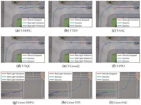
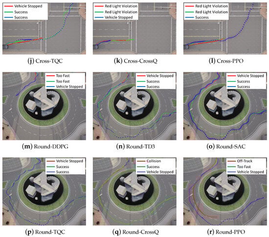
Figure 8.
Comparison of driving performance at T-, Cross-, and Round-Intersections for each algorithm. For each RL algorithm, its driving trajectories at different training stages are visualized (green for 200 k steps, red for 600 k steps, and blue for 1 M steps). The legend indicates the success or failure of each trajectory, and in cases of failure, the cause of failure is also specified.
The DDPG algorithm demonstrated a relatively stable driving performance on straight roads; however, it consistently failed across all intersection types, even as training progressed. This instability is attributed to the increasing difficulty of accurately estimating Q-values in more complex traffic scenarios, which amplifies Q-value overestimation and undermines policy reliability. While PPO mitigates Q-value overestimation to some extent and succeeded in the T- and Cross-Intersections as training advanced, it failed to navigate the Round-Intersection even after 1M training steps. CrossQ showed partial success in the Round-Intersection scenario but repeatedly failed at the T- and Cross-Intersections with traffic lights, displaying similar tendencies to those of DDPG.
In contrast, TD3, SAC, and TQC successfully completed all intersection tasks after approximately 600k training steps. This success is interpreted as being a result of their double critic structures, which suppress Q-value overestimation, and their entropy-based exploration strategies, which facilitate stable policy learning even in complex environments.
These results collectively suggest that successful intersection navigation in urban environments relies not only on expressive state representations but also, critically, on the exploration strategy and stability of Q-value estimation within the DRL algorithm.
6.1. Evaluation of Driving Performance
Table 8 presents a comparative analysis of each algorithm in terms of three key navigation metrics: Travel Distance, Route Completion, and Success Rate.
Table 8.
Metrics for evaluating driving performance after 1 M steps of learning (Bold text indicates the method that achieves the best performance for each metric).
TQC achieved the best performance across all three navigation metrics. Notably, its Success Rate reached 80%, indicating that the learned policy was capable of consistently completing routes under diverse road conditions.
SAC exhibited a comparable performance to TQC in terms of Travel Distance and Route Completion, but its Success Rate was slightly lower, at approximately 65%. This suggests that while SAC displayed robust route-following behavior, it may have encountered penalties that led to task failures. Similarly, TD3 showed a reasonably high Route Completion of 77%, yet its Success Rate dropped to 60%, highlighting limitations in its generalization or rule adherence.
In contrast, both CrossQ and DDPG demonstrated significantly lower values in Route Completion and Success Rate. In particular, both algorithms recorded a Success Rate of 0%, indicating a complete failure in mission completion.
Overall, the results suggest that a higher Travel Distance and Route Completion generally correlate to a higher Success Rate. Since the Success Rate reflects full Route Completion, while Travel Distance and Route Completion represent partial progress, the latter two can be seen as necessary, but not sufficient, conditions. Completing a full route successfully requires further policies that incorporate the robust handling of traffic regulations and lane-keeping across the entire route.
6.2. Evaluation of Reward-Based Performances
Table 9 presents a comparative analysis of the reward-based performance of each algorithm in terms of Episode Reward Mean, Step Reward Mean, and Reward Standard Deviation.
Table 9.
Performance comparison of reward-based metrics over 1 M steps of learning (Bold text indicates the method that achieves the best performance for each metric).
TQC consistently outperformed all other algorithms across these three metrics. It achieved the highest Episode Reward Mean of 977.7 and the highest Step Reward Mean of 0.62. Additionally, it recorded the lowest Reward Standard Deviation of 0.28, indicating that the learned policy was capable of acquiring rewards in a stable and consistent manner at each time step. This suggests that TQC’s distributional reinforcement learning framework effectively minimized reward volatility while maximizing reward gains, even under uncertain autonomous driving scenarios.
SAC ranked second in both Episode Reward Mean and Step Reward Mean, closely following TQC. It also maintained a relatively low Reward Standard Deviation of 0.33, demonstrating good stability in reward acquisition throughout each episode.
TD3 performed moderately well in the reward-related metrics. Although its Reward Standard Deviation (0.31) was slightly lower than SAC’s, it fell behind in terms of total reward accumulation, reflected in its lower values for Episode Reward Mean and Step Reward Mean. PPO produced a similar level of mean rewards to TD3 but exhibited a higher Reward Standard Deviation of 0.40, indicating greater variability and suggesting that PPO’s on-policy nature led to less stable policy updates during training.
CrossQ and DDPG recorded relatively poor performance across all reward-based metrics. However, CrossQ outperformed DDPG in all three indicators, Episode Reward Mean, Step Reward Mean, and Reward Standard Deviation, implying that CrossQ achieved relatively improved policy optimization over DDPG despite its overall low Route Completion performance.
6.3. Evaluation of Driving Stability, Efficiency, and Comfort
Table 10 compares the performance of various DRL algorithms in terms of Centerline Deviation Mean and Speed Mean, which represent their lane-keeping stability and driving efficiency, respectively.
Table 10.
Performance comparison of Centerline Deviation Mean and Speed Mean across DRL algorithms over 1 M steps of learning (Bold text indicates the method that achieves the best performance for each metric).
It is important to note that these two metrics often exhibit an inverse relationship. A higher Speed Mean may lead to an increased Centerline Deviation Mean due to the influence of vehicular inertia, particularly during curved driving. However, excessively reducing the speed to maintain center alignment can degrade driving efficiency. Therefore, an optimal trade-off between stability and efficiency must be maintained, as encouraged through reward function’s design.
TQC achieved the lowest Centerline Deviation Mean of 0.11, indicating its superior ability to maintain alignment with the lane center throughout the driving episodes. SAC followed closely with a deviation of 0.16, also demonstrating effective and stable lane-keeping behavior.
CrossQ, TD3, and PPO recorded deviations of 0.18, 0.19, and 0.20, respectively, reflecting their moderate performance in terms of lateral control. Notably, CrossQ exhibited relatively favorable lane-keeping stability despite its overall low Route Completion performance, which is a noteworthy observation.
In contrast, DDPG recorded the highest Centerline Deviation Mean of 0.41, suggesting significant deviation from the center of the lane. This outcome highlights a severe limitation in DDPG’s ability to maintain stable vehicle alignment.
Driving speed, represented by Speed Mean, encapsulates aspects of both driving efficiency and passenger comfort [78]. In terms of efficiency—and excluding DDPG—TD3, TQC, and CrossQ exhibited the highest performance. The fact that TQC simultaneously maintained excellent lane stability and a high average speed underscores its overall effectiveness in balancing safety and efficiency.
On the other hand, DDPG showed an abnormally high average speed combined with poor lateral control, implying a potentially uncomfortable and erratic driving experience for passengers. This suggests that DDPG may not be suitable for deployment in scenarios requiring both safety and ride comfort.
6.4. Analysis of Penalty and Failure Factors
Table 11 and Table 12 present a quantitative comparison of the occurrence rates of five penalty types—vehicle stopped, off-track, too fast, red light violation, and collision—across different DRL algorithms and simulated towns.
Table 11.
Results of analysis of penalty factors according to the DRL algorithm tested. (Bold text indicates the method that achieves the best performance for each metric).
Table 12.
Results of analysis of penalty factors across different towns. (Bold text indicates the town with the highest penalty for each metric).
Among all algorithms, the most frequently triggered penalty was vehicle stopped, followed by red light violation. The vehicle stopped penalty was typically induced when a vehicle failed to proceed after a green signal or unnecessarily halted upon detecting a traffic light despite it displaying a go signal. Additionally, in many cases, vehicles misinterpreted the road structure—particularly in complex or nonlinear layouts—and stopped inappropriately even when a red light was correctly detected.
Both TQC and SAC achieved the lowest penalty rates across all categories, indicating that these algorithms effectively learned driving policies that balance both road-rule compliance and trajectory stability.
In contrast, CrossQ recorded the highest overall penalty rates, with especially high frequencies in the vehicle stopped (0.69) and too fast (0.29) categories. These shortcomings can be attributed to CrossQ’s architectural design. Unlike standard actor–critic frameworks, CrossQ eliminates the use of a target network to enhance sampling efficiency and reduce computational cost, instead employing Batch Renormalization within the critic network. While this design promotes faster convergence and structural simplicity, it comes at the cost of omitting stabilizing mechanisms like target networks, making it vulnerable to Q-value overestimation and reduced policy robustness in challenging driving environments, such as signalized intersections. Previous research has also reported a tendency for CrossQ to exhibit a higher Q-function bias—including overestimation—than other algorithms [35], which aligns with the unstable performance and elevated penalty rates observed in our study.
Town03 yielded the highest penalty rates among all environments. Specifically, its roundabout sections posed challenges for directional perception, often leading to vehicle stopped penalties. Moreover, off-track and too fast penalties were also quite frequent in Town03, likely due to the increased difficulty of maintaining lane discipline and speed control while navigating complex circular intersections.
Town05, characterized by the largest number of signalized intersections, showed the highest incidence of red light violations. Meanwhile, although Town01 has a relatively simple urban layout, its longer routes increased the likelihood of encountering penalty events during extended navigation. In contrast, Town02, which served as the training environment, recorded the lowest penalty rates across all categories. This highlights the importance of focused pretraining in the target deployment domain to improve operational safety and compliance in autonomous driving systems.
In summary, the penalty analysis reveals that beyond overall Success Rate, significant variability exists in rule adherence and stability performance across both algorithmic designs and simulation environments. Notably, the presence of complex road structures and rule-based elements amplifies the differences among DRL models and underscores the critical impact of pretraining strategies in minimizing penalty risks.
7. Conclusions
To enable autonomous driving under a diverse range of real-world geographic variations and complex traffic regulations, this study conducted a comparative analysis of the best driving policy algorithms based on DRL within a closed-loop CARLA simulator framework. Six representative DRL algorithms—DDPG, SAC, TD3, PPO, TQC, and CrossQ—were selected as benchmark methods, and custom-designed reward and penalty functions were formulated and integrated into the experiment to reflect various situational factors. Our experimental results demonstrate that off-policy methods that maximize sample efficiency and employ stochastic policies, particularly TQC and SAC, achieve the most effective learning performance. It was also observed that geographically variant elements within the towns—such as traffic lights, intersections, and roundabouts—as well as their corresponding regulatory constraints, acted as degradation factors in metrics such as Route Completion, Success Rate, and Centerline Deviation Mean. For instance, Route Completion improved from 0.23 with DDPG to 0.91 with TQC, while the Success Rate increased from 0.0 with DDPG to 0.8 with TQC. These results highlight that the challenges introduced by environmental variation and rule compliance can be effectively addressed using DRL approaches like SAC and TQC, which mitigate the Q-value overestimation problem via statistical learning techniques. Nevertheless, despite the relative stability of TQC and SAC, certain limitations persist—especially in areas such as precise stop-point determination under various traffic light scenarios and the modulation of optimal speeds to prevent abrupt acceleration or deceleration.
8. Future Work
In future research, we plan to extend our study to more realistic autonomous driving scenarios that involve dynamic and heterogeneous traffic environments, including varying levels of vehicle density and the presence of pedestrian crossings. By incorporating such traffic conditions, we aim to assess the performance of the current DRL algorithms as well as develop improved versions capable of robust decision-making in complex real-world contexts.
Additionally, we will explore a Sim-to-Real transfer pipeline by adapting the DRL-based optimal policy network, which has been validated in the CARLA simulator, to real-world data. This will involve modeling data distribution shifts and conducting thorough performance evaluations to ensure the generalizability and applicability of the trained policies to physical driving platforms.
Furthermore, we intend to design a novel reward function that incorporates differentiated importance weights for each step and episode. This approach aims to better reflect the safety-critical nature of autonomous driving by assigning higher significance to decision points that have greater influence on safety during driving.
Finally, we will investigate the applicability of emerging reinforcement learning algorithms to autonomous driving. In particular, we aim to explore model-based methods such as DreamerV3 [79], off-policy methods with auxiliary tasks like SAC-X [80], generative policy learning using Diffusion Policy [81], and generalist transformer-based architectures such as Gato [82]. These advanced techniques offer the potential for improved sample efficiency, multi-modal decision modeling, and scalability across diverse driving tasks.
Author Contributions
Conceptualization, Y.P. and S.L.; methodology, Y.P.; software, Y.P.; validation, Y.P., W.J. and S.L.; formal analysis, S.L.; investigation, S.L.; resources, S.L.; data curation, Y.P. and W.J.; writing—original draft preparation, S.L.; writing—review and editing, S.L.; visualization, Y.P.; supervision, S.L.; project administration, S.L.; funding acquisition, S.L. All authors have read and agreed to the published version of the manuscript.
Funding
This work was supported by the Soonchunhyang University Research Fund (No. 20250561).
Institutional Review Board Statement
Not applicable.
Informed Consent Statement
Not applicable.
Data Availability Statement
The original contributions presented in this study are included in the article. Further inquiries can be directed to the corresponding author.
Conflicts of Interest
The authors declare no conflicts of interest.
References
- Krizhevsky, A.; Sutskever, I.; Hinton, G.E. ImageNet Classification with Deep Convolutional Neural Networks. In Proceedings of the 25th International Conference on Neural Information Processing Systems (NeurIPS), Lake Tahoe, NV, USA, 3–8 December 2012. [Google Scholar]
- He, K.; Zhang, X.; Ren, S.; Sun, J. Deep Residual Learning for Image Recognition. In Proceedings of the IEEE Conference on Computer Vision and Pattern Recognition (CVPR), Las Vegas, NV, USA, 27–30 June 2016. [Google Scholar]
- Vaswani, A.; Shazeer, N.; Parmar, N.; Uszkoreit, J.; Jones, L.; Gomez, A.N.; Kaiser, L.; Polosukhin, I. Attention Is All You Need. In Proceedings of the 30th International Conference on Neural Information Processing Systems (NeurIPS), Long Beach, CA, USA, 4–9 December 2017. [Google Scholar]
- Deng, J.; Dong, W.; Socher, R.; Li, L.-J.; Li, K.; Li, F.-F. ImageNet: A large-scale hierarchical image database. In Proceedings of the IEEE Conference on Computer Vision and Pattern Recognition (CVPR), Miami, FL, USA, 20–25 June 2009. [Google Scholar]
- Geiger, A.; Lenz, P.; Urtasun, R. Are we ready for Autonomous Driving? The KITTI Vision Benchmark Suite. In Proceedings of the IEEE Conference on Computer Vision and Pattern Recognition (CVPR), Providence, RI, USA, 16–21 June 2012. [Google Scholar]
- Caesar, H.; Bankiti, V.; Lang, A.H.; Vora, S.; Liong, V.E.; Xu, Q.; Krishnan, A.; Pan, Y.; Baldan, G.; Beijbom, O. nuScenes: A multimodal dataset for autonomous driving. In Proceedings of the Computer Vision and Pattern Recognition (CVPR), Seattle, WA, USA, 14–19 June 2020. [Google Scholar]
- Jun, W.; Lee, S. A Comparative Study and Optimization of Camera-Based BEV Segmentation for Real-Time Autonomous Driving. Sensors 2025, 25, 2300. [Google Scholar] [CrossRef] [PubMed]
- Kwak, D.; Yoo, J.; Son, M.; Park, M.; Choi, D.; Lee, S. Rethinking Real-Time Lane Detection Technology for Autonomous Driving. J. Korean Inst. Commun. Inf. Sci. 2023, 48, 589–599. [Google Scholar] [CrossRef]
- Cheong, Y.; Jun, W.; Lee, S. Study on Point Cloud Based 3D Object Detection for Autonomous Driving. J. Korean Inst. Commun. Inf. Sci. 2024, 49, 31–40. [Google Scholar] [CrossRef]
- Jun, W.; Yoo, J.; Lee, S. Synthetic Data Enhancement and Network Compression Technology of Monocular Depth Estimation for Real-Time Autonomous Driving System. Sensors 2024, 24, 4205. [Google Scholar] [CrossRef]
- Jun, W.; Lee, S. Optimal Configuration of Multi-Task Learning for Autonomous Driving. Sensors 2023, 23, 9729. [Google Scholar] [CrossRef]
- Son, M.; Won, Y.; Lee, S. Optimizing Large Language Models: A Deep Dive into Effective Prompt Engineering Techniques. Appl. Sci. 2025, 15, 1430. [Google Scholar] [CrossRef]
- Son, M.; Lee, S. Advancing Multimodal Large Language Models: Optimizing Prompt Engineering Strategies for Enhanced Performance. Appl. Sci. 2025, 15, 3992. [Google Scholar] [CrossRef]
- Yang, Z.; Jia, X.; Li, H.; Yan, J. LLM4Drive: A Survey of Large Language Models for Autonomous Driving. arXiv 2023, arXiv:2311.01043. [Google Scholar]
- Cui, C.; Ma, Y.; Cao, X.; Ye, W.; Zhou, Y.; Liang, K.; Chen, J.; Lu, J.; Yang, Z.; Liao, K.; et al. A Survey on Multimodal Large Language Models for Autonomous Driving. In Proceedings of the IEEE/CVF Winter Conference on Applications of Computer Vision (WACV), Waikoloa, HI, USA, 2–6 January 2024; pp. 958–979. [Google Scholar]
- Choi, J.; Park, Y.; Jun, W.; Lee, S. Research Trends Focused on End-to-End Learning Technologies for Autonomous Vehicles. J. Korean Inst. Commun. Inf. Sci. 2024, 49, 1614–1630. [Google Scholar] [CrossRef]
- Ye, F.; Zhang, S.; Wang, P.; Chan, C. A Survey of Deep Reinforcement Learning Algorithms for Motion Planning and Control of Autonomous Vehicles. In Proceedings of the 2021 IEEE Intelligent Vehicles Symposium (IV), Nagoya, Japan, 11–13 July 2021. [Google Scholar]
- Zhao, R.; Li, Y.; Fan, Y.; Gao, F.; Tsukada, M.; Gao, Z. A Survey on Recent Advancements in Autonomous Driving Using Deep Reinforcement Learning: Applications, Challenges, and Solutions. IEEE Trans. Intell. Transp. Syst. 2024, 25, 19365–19398. [Google Scholar] [CrossRef]
- Zhu, Z.; Zhao, H. A Survey of Deep RL and IL for Autonomous Driving Policy Learning. IEEE Trans. Intell. Transp. Syst. 2021, 23, 14043–14065. [Google Scholar] [CrossRef]
- Dinneweth, J.; Boubezoul, A.; Mandiau, R.; Espié, S. Multi-agent reinforcement learning for autonomous vehicles: A survey. Auton. Intell. Syst. 2022, 2, 27. [Google Scholar] [CrossRef]
- Wu, J.; Huang, C.; Huang, H.; Lv, C.; Wang, Y.; Wang, F. Recent advances in reinforcement learning-based autonomous driving behavior planning: A survey. Transp. Res. Part Emerg. Technol. 2024, 164, 104654. [Google Scholar] [CrossRef]
- Ross, S.; Gordon, G.J.; Bagnell, J.A. A Reduction of Imitation Learning and Structured Prediction to No-Regret Online Learning. In Proceedings of the 14th International Conference on Artificial Intelligence and Statistics (AISTATS 2011), Fort Lauderdale, FL, USA, 11–13 April 2011; Volume 15, pp. 627–635. [Google Scholar]
- Ross, S.; Bagnell, D. Efficient Reductions for Imitation Learning. In Proceedings of the 13th International Conference on Artificial Intelligence and Statistics (AISTATS 2010), Chia Laguna Resort, Italy, 13–15 May 2010; Volume 9, pp. 661–668. [Google Scholar]
- Wu, Y.-H.; Charoenphakdee, N.; Bao, H.; Tangkaratt, V.; Sugiyama, M. Imitation Learning from Imperfect Demonstration. In Proceedings of the 36th International Conference on Machine Learning (ICML 2019), Long Beach, CA, USA, 9–15 June 2019; PMLR: London, UK, 2019; Volume 97, pp. 6818–6827. [Google Scholar]
- Codevilla, F.; Muller, M.; Lopez, A.; Koltun, V.; Dosovitskiy, A. End-to-End Driving via Conditional Imitation Learning. In Proceedings of the International Conference on Robotics and Automation (ICRA), Brisbane, QLD, Australia, 21–25 May 2018; IEEE: Piscataway, NJ, USA, 2018; pp. 4693–4700. [Google Scholar]
- Ho, J.; Ermon, S. Generative Adversarial Imitation Learning (GAIL). In Proceedings of the 30th Conference on Neural Information Processing Systems (NeurIPS), Barcelona, Spain, 5–10 December 2016. [Google Scholar]
- Chen, L.; Wu, P.; Chitta, K.; Jaeger, B.; Geiger, A.; Li, H. End-to-end Autonomous Driving: Challenges and Frontiers. IEEE Trans. Pattern Anal. Mach. Intell. 2024, 46, 10164–10183. [Google Scholar] [CrossRef]
- Mnih, V.; Kavukcuoglu, K.; Silver, D.; Graves, A.; Antonoglou, I.; Wierstra, D.; Riedmiller, M. Playing Atari with Deep Reinforcement Learning. In Proceedings of the NIPS Deep Learning Workshop 2013, Lake Tahoe, NV, USA, 6–7 December 2013. [Google Scholar]
- Mnih, V.; Badia, A.P.; Mirza, M.; Graves, A.; Lillicrap, T.P.; Harley, T.; Silver, D.; Kavukcuoglu, K. Asynchronous Methods for Deep Reinforcement Learning. arXiv 2016, arXiv:1602.01783. [Google Scholar]
- Schulman, J.; Wolski, F.; Dhariwal, P.; Radford, A.; Klimov, O. Proximal Policy Optimization Algorithms. arXiv 2017, arXiv:1707.06347. [Google Scholar]
- Schulman, J.; Levine, S.; Moritz, P.; Jordan, M.I.; Abbeel, P. Trust Region Policy Optimization. In Proceedings of the 32nd International Conference on Machine Learning (ICML), Lille, France, 6–11 July 2015. [Google Scholar]
- Lillicrap, T.P.; Hunt, J.J.; Pritzel, A.; Heess, N.; Erez, T.; Tassa, Y.; Silver, D.; Wierstra, D. Continuous Control with Deep Reinforcement Learning. arXiv 2015, arXiv:1509.02971. [Google Scholar]
- Fujimoto, S.; Hoof, H.; Meger, D. Addressing Function Approximation Error in Actor-Critic Methods. In Proceedings of the 35th International Conference on Machine Learning (ICML), Stockholm, Sweden, 10–15 July 2018; PMLR: London, UK, 2018; pp. 1587–1596. [Google Scholar] [CrossRef]
- Haarnoja, T.; Zhou, A.; Abbeel, P.; Levine, S. Soft Actor-Critic: Off-Policy Maximum Entropy Deep Reinforcement Learning with a Stochastic Actor. In Proceedings of the 35th International Conference on Machine Learning (ICML), Stockholm, Sweden, 10–15 July 2018; PMLR: London, UK, 2018; pp. 1861–1870. [Google Scholar] [CrossRef]
- Bhatt, A.; Rhinehart, N.; Levine, S. CrossQ: Batch Normalization in Deep Reinforcement Learning for Greater Sample Efficiency and Simplicity. arXiv 2019, arXiv:1902.05605. [Google Scholar]
- Kuznetsov, A.; Laskin, M.; Kostrikov, I.; Abbeel, P. Controlling Overestimation Bias with Truncated Mixture of Continuous Distributional Quantile Critics. In Proceedings of the 37th International Conference on Machine Learning (ICML), Vienna, Austria, 12–18 July 2020; PMLR: London, UK, 2020. [Google Scholar] [CrossRef]
- Li, D.; Okhrin, O. Modified DDPG car-following model with a real-world human driving experience with CARLA simulator. Transp. Res. Part 2023, 147, 103987. [Google Scholar] [CrossRef]
- Jumman Hossain, Autonomous Driving with Deep Reinforcement Learning in CARLA Simulation. arXiv 2023, arXiv:2306.11217.
- Sharma, R.; Garg, P. Optimizing Autonomous Driving with Advanced Reinforcement Learning: Evaluating DQN and PPO. In Proceedings of the 5th International Conference on Smart Electronics and Communication (ICOSEC), Tiruchirappalli, India, 18–20 September 2024. [Google Scholar]
- Pérez-Gil, Ó.; Barea, R.; López-Guillén, E.; Bergasa, L.M.; Gómez-Huélamo, C.; Gutiérrez, R.; Díaz-Díaz, A. Deep reinforcement learning based control for Autonomous Vehicles in CARLA. Multimed. Tools Appl. 2022, 81, 3553–3576. [Google Scholar] [CrossRef]
- Dosovitskiy, A.; Ros, G.; Codevilla, F.; Lopez, A.; Koltun, V. CARLA: An Open Urban Driving Simulator. In Proceedings of the 1st Annual Conference on Robot Learning (CoRL), Mountain View, CA, USA, 13–15 November 2017; PMLR: London, UK, 2017; Volume 78, pp. 1–16. [Google Scholar] [CrossRef]
- Pomerleau, D.A. ALVINN: An Autonomous Land Vehicle in a Neural Network. In Proceedings of the 1st International Conference on Neural Information Processing Systems (NIPS), Denver, CO, USA, 27–30 December 1988; pp. 305–313. [Google Scholar]
- Bojarski, M.; Testa, D.D.; Dworakowski, D.; Firner, B.; Flepp, B.; Goyal, P.; Jackel, L.D.; Monfort, M.; Muller, U.; Zhang, J.; et al. End to End Learning for Self-Driving Cars. arXiv 2016, arXiv:1604.07316. [Google Scholar]
- Rhinehart, N.; McAllister, R.; Levine, S. Deep Imitative Models for Flexible Inference, Planning, and Control. In Proceedings of the IEEE/CVF Conference on Computer Vision and Pattern Recognition (CVPR), Salt Lake City, UT, USA, 18–22 June 2018; pp. 8001–8009. [Google Scholar]
- Kim, S.; Shin, J. Deep Imitation Learning for End-to-End Autonomous Driving: Integration of Carla and OpenAI Gym. In Proceedings of the 5th International Conference on Smart Electronics and Communication (ICOSEC), Tiruchirappalli, India, 18–20 September 2024. [Google Scholar]
- Shi, J.; Zhang, T.; Zhan, J.; Chen, S.; Xin, J.; Zheng, N. Efficient Lane-changing Behavior Planning via Reinforcement Learning with Imitation Learning Initialization. In Proceedings of the IEEE Intelligent Vehicles Symposium (IV), Anchorage, AK, USA, 4–7 June 2023. [Google Scholar]
- Lu, Y.; Fu, J.; Tucker, G.; Pan, X.; Bronstein, E.; Roelofs, R.; Sapp, B.; White, B.; Faust, A.; Whiteson, S.; et al. Imitation Is Not Enough: Robustifying Imitation with Reinforcement Learning for Challenging Driving Scenarios. arXiv 2022, arXiv:2212.11419. [Google Scholar]
- Nehme, G.; Deo, T.Y. Safe Navigation: Training Autonomous Vehicles using Deep Reinforcement Learning in CARLA. arXiv 2023, arXiv:2311.10735. [Google Scholar]
- Khlifi, A.; Othmani, M.; Kherallah, M. A Novel Approach to Autonomous Driving Using Double Deep Q-Network-Based Deep Reinforcement Learning. World Electr. Veh. J. 2025, 16, 138. [Google Scholar] [CrossRef]
- Terapaptommakol, W.; Phaoharuhansa, D.; Koowattanasuchat, P.; Rajruangrabin, J. Design of Obstacle Avoidance for Autonomous Vehicle Using Deep Q-Network and CARLA Simulator. World Electr. Veh. J. 2022, 13, 239. [Google Scholar] [CrossRef]
- Cai, P.; Wang, S.; Wang, H.; Liu, M. Carl-Lead: Lidar-based End-to-End Autonomous Driving with Contrastive Deep Reinforcement Learning. arXiv 2021, arXiv:2109.08473v1. [Google Scholar]
- Elallid, B.B.; Benamar, N.; Mrani, N.; Rachidi, T. DQN-based Reinforcement Learning for Vehicle Control of Autonomous Vehicles Interacting With Pedestrians. In Proceedings of the 2022 International Conference on Innovation and Intelligence for Informatics, Computing, and Technologies (3ICT), Sakhir, Bahrain, 22–23 November 2022. [Google Scholar]
- Li, G.; Yanga, Y.; Li, S.; Qu, X.; Lyuc, N.; Li, S.E. Decision making of autonomous vehicles in lane change scenarios: Deep reinforcement learning approaches with risk awareness. Transp. Res. Part C 2022, 134, 103452. [Google Scholar] [CrossRef]
- Liang, X.; Wang, T.; Yang, L.; Xing, E. CIRL: Controllable Imitative Reinforcement Learning for Vision-based Self-driving. In Proceedings of the 15th European Conference on Computer Vision (ECCV), Munich, Germany, 8–14 September 2018; Springer: Cham, Switzerland, 2018; Volume 11206, pp. 584–599. [Google Scholar]
- Činčurak, D.; Grbić, R.; Vranješ, M.; Vranješ, D. Autonomous Vehicle Control in CARLA Simulator using Reinforcement Learning. In Proceedings of the 66th International Symposium ELMAR-2024, Zadar, Croatia, 16–18 September 2024. [Google Scholar]
- Perez-Gil, O.; Barea, R.; Lopez-Guillen, E.; Bergasa, L.M.; Gomez-Huelamo, C.; Gutierrez, R.; Diaz, A. Deep Reinforcement Learning Based Control Algorithms: Training and Validation Using the ROS Framework in CARLA Simulator for Self-Driving Applications. In Proceedings of the 2021 IEEE Intelligent Vehicles Symposium (IV), Nagoya, Japan, 11–17 July 2021; IEEE: New York, NY, USA; pp. 958–963. [Google Scholar]
- Ahmed, M.; Abobakr, A.; Lim, C.P.; Nahavandi, S. Policy-Based Reinforcement Learning for Training Autonomous Driving Agents in Urban Areas With Affordance Learning. IEEE Trans. Intell. Transp. Syst. 2022, 23, 12562–12571. [Google Scholar] [CrossRef]
- Matsioris, G.; Theocharous, A.; Tsourveloudis, N.; Doitsidis, L. Towards developing a framework for autonomous electric vehicles using CARLA: A Validation using the Deep Deterministic Policy Gradient algorithm. In Proceedings of the 2024 32nd Mediterranean Conference on Control and Automation (MED), Chania, Greece, 11–14 June 2024. [Google Scholar]
- Huang, C.; Zhang, R.; Ouyang, M.; Wei, P.; Lin, J.; Su, J.; Lin, L. Deductive Reinforcement Learning for Visual Autonomous Urban Driving Navigation. IEEE Trans. Neural Netw. Learn. Syst. 2021, 32, 5379–5391. [Google Scholar] [CrossRef] [PubMed]
- Anzalone, L.; Barra, S.; Nappi, M. Reinforced Curriculum Learning for Autonomous Driving in CARLA. In Proceedings of the 2021 IEEE International Conference on Image Processing (ICIP), Anchorage, AK, USA, 19–22 September 2021; IEEE: Piscataway, NJ, USA, 2021. [Google Scholar]
- Gutiérrez-Moreno, R.; Barea, R.; López-Guillén, E.; Araluce, J.; Bergasa, L.M. Reinforcement Learning-Based Autonomous Driving at Intersections in CARLA Simulator. Sensors 2022, 22, 8373. [Google Scholar] [CrossRef]
- Wang, L.; Liu, J.; Shao, H.; Wang, W.; Chen, R.; Liu, Y.; Waslander, S.L. Efficient Reinforcement Learning for Autonomous Driving with Parameterized Skills and Priors. In Proceedings of the Robotics: Science and Systems (RSS), Daegu, Republic of Korea, 10–14 July 2023; PMLR: Cambridge, MA, USA, 2023. [Google Scholar]
- Siboo, S.; Bhattacharyya, A.; Raj, R.N.; Ashwin, S.H. An Empirical Study of DDPG and PPO-Based Reinforcement Learning Algorithms for Autonomous Driving. IEEE Access 2023, 11, 125094–125108. [Google Scholar] [CrossRef]
- Pei, X.; Mo, S.; Chen, Z.; Yang, B. Lane Changing of Autonomous Vehicle Based on TD3 algorithm in Human-machine Hybrid Driving Environment. China J. Highw. Transp. 2021, 34, 246–254. [Google Scholar]
- Elallid, B.B.; Alaoui, H.E.; Benamar, N. Deep Reinforcement Learning for Autonomous Vehicle Intersection Navigation. In Proceedings of the 2023 International Conference on Innovation and Intelligence for Informatics, Computing, and Technologies (3ICT), Sakhir, Bahrain, 20–23 November 2023; IEEE: New York, NY, USA, 2023. [Google Scholar]
- Liua, Y.; Gaoc, Y.; Zhanga, Q.; Dingc, D.; Zhao, D. Multi-task Safe Reinforcement Learning for Navigating Intersections in Dense Traffic. J. Frankl. Inst. 2023, 360, 13737–13760. [Google Scholar] [CrossRef]
- Wang, K.; She, C.; Li, Z.; Yu, T.; Li, Y.; Sakaguchi, K. Roadside Units Assisted Localized Automated Vehicle Maneuvering: An Offline Reinforcement Learning Approach. arXiv 2024, arXiv:2405.03935. [Google Scholar]
- Liu, Q.; Dang, F.; Wang, X.; Ren, X. Autonomous Highway Merging in Mixed Traffic Using Reinforcement Learning and Motion Predictive Safety Controller. In Proceedings of the 2022 IEEE 25th International Conference on Intelligent Transportation Systems (ITSC), Macau, China, 8–12 October 2022; pp. 1063–1069. [Google Scholar]
- Elallid, B.B.; Benamar, N.; Bagaa, M.; Hadjadj-Aoul, Y. Enhancing Autonomous Driving Navigation Using Soft Actor-Critic. Future Internet 2024, 16, 238. [Google Scholar] [CrossRef]
- Aghdasian, A.J.; Ardakani, A.H.; Aqabakee, K.; Abdollahi, F. Autonomous Driving using Residual Sensor Fusion and Deep Reinforcement Learning. In Proceedings of the 2023 11th RSI International Conference on Robotics and Mechatronics (ICRoM), Tehran, Iran, 13–15 December 2023; pp. 265–270. [Google Scholar]
- Abdollahian, S.A.; Fazel, S.; Hadadi, M.R.; Aghdasian, A.J. Enhancing Autonomous Vehicle Control through Sensor Fusion, NARX-based Reinforcement Learning with Soft Actor-Critic (SAC) in CARLA Simulator. In Proceedings of the RoboCup 2024: Robot World Cup XXVII, Cham, Switzerland, 15–22 July 2024; pp. 224–235. [Google Scholar]
- Yao, F.; Sun, C.; Lu, B.; Wang, B.; Yu, H. Mixture of Experts Framework Based on Soft Actor-Critic algorithm for Highway Decision-Making of Connected and Automated Vehicles. Chin. J. Mech. Eng. 2025, 38, 1. [Google Scholar] [CrossRef]
- Hart, P.E.; Nilsson, N.J.; Raphael, B. A formal basis for the heuristic determination of minimum cost paths. IEEE Trans. Syst. Sci. Cybern. 1968, 4, 100–107. [Google Scholar] [CrossRef]
- Feng, Y.; Zhang, W.; Zhu, J. Application of an improved A* algorithm for the path analysis of urban multi-type transportation systems. Appl. Sci. 2023, 13, 13090. [Google Scholar] [CrossRef]
- Wang, S.; Wang, Z.; Wang, X.; Liang, Q.; Meng, L. Intelligent vehicle driving decision-making model based on variational AutoEncoder network and deep reinforcement learning. Expert Syst. Appl. 2025, 268, 126319. [Google Scholar] [CrossRef]
- Azizpour, M.; da Roza, F.; Bajcinca, N. End-to-end autonomous driving controller using semantic segmentation and variational autoencoder. In Proceedings of the 2020 7th International Conference on Control, Decision and Information Technologies (CoDIT), Prague, Czech Republic, 29 June–2 July 2020; IEEE: New York, NY, USA, 2020; Volume 1, pp. 1075–1080. [Google Scholar]
- Diaz-Diaz, A.; Aranda, M.; Barea, R.; Bergasa, L.M.; Arroyo, R. HD Maps: Exploiting OpenDRIVE Potential for Path Planning and Map Monitoring. In Proceedings of the 2022 IEEE Intelligent Vehicles Symposium (IV), Aachen, Germany, 5–9 June 2022; IEEE: New York, NY, USA, 2022; pp. 1211–1217. [Google Scholar] [CrossRef]
- Jung, S.; Jun, W.; Oh, T.; Lee, S. Performance Analysis of Motion Planning for Outdoor Autonomous Delivery Robot. In Proceedings of the 2024 IEEE International Conference on Consumer Electronics (ICCE), Las Vegas, NV, USA, 6–8 January 2024; IEEE: New York, NY, USA, 2024; pp. 1–6. [Google Scholar]
- Hafner, D.; Lillicrap, T.; Ba, J.; Norouzi, M. Mastering Diverse Domains through World Models. arXiv 2023, arXiv:2301.04104. [Google Scholar]
- Riedmiller, M.; Hafner, R.; Lampe, T.; Neunert, M.; Degrave, J.; de Wiele, T.V.; Mnih, V.; Heess, N.; Springenberg, T. Learning by Playing: Solving Sparse Reward Tasks from Scratch. In Proceedings of the 35th International Conference on Machine Learning (ICML), Stockholm, Sweden, 10–15 July 2018; PMLR: Cambridge, MA, USA, 2018; Volume 80, pp. 4344–4353. [Google Scholar]
- Chi, C.; Xu, Z.; Feng, S.; Cousineau, E.; Du, Y.; Burchfiel, B.; Tedrake, R.; Song, S. Diffusion Policy: Visuomotor Policy Learning via Action Diffusion. Int. J. Robot. Res. 2024; Online First. [Google Scholar] [CrossRef]
- Reed, S.; Żołna, K.; Parisotto, E.; Colmenarejo, S.G.; Novikov, A.; Barth-Maron, G.; Giménez, M.; Sulsky, Y.; Kay, J.; Springenberg, J.T.; et al. A Generalist Agent. arXiv 2022, arXiv:2205.06175. [Google Scholar]
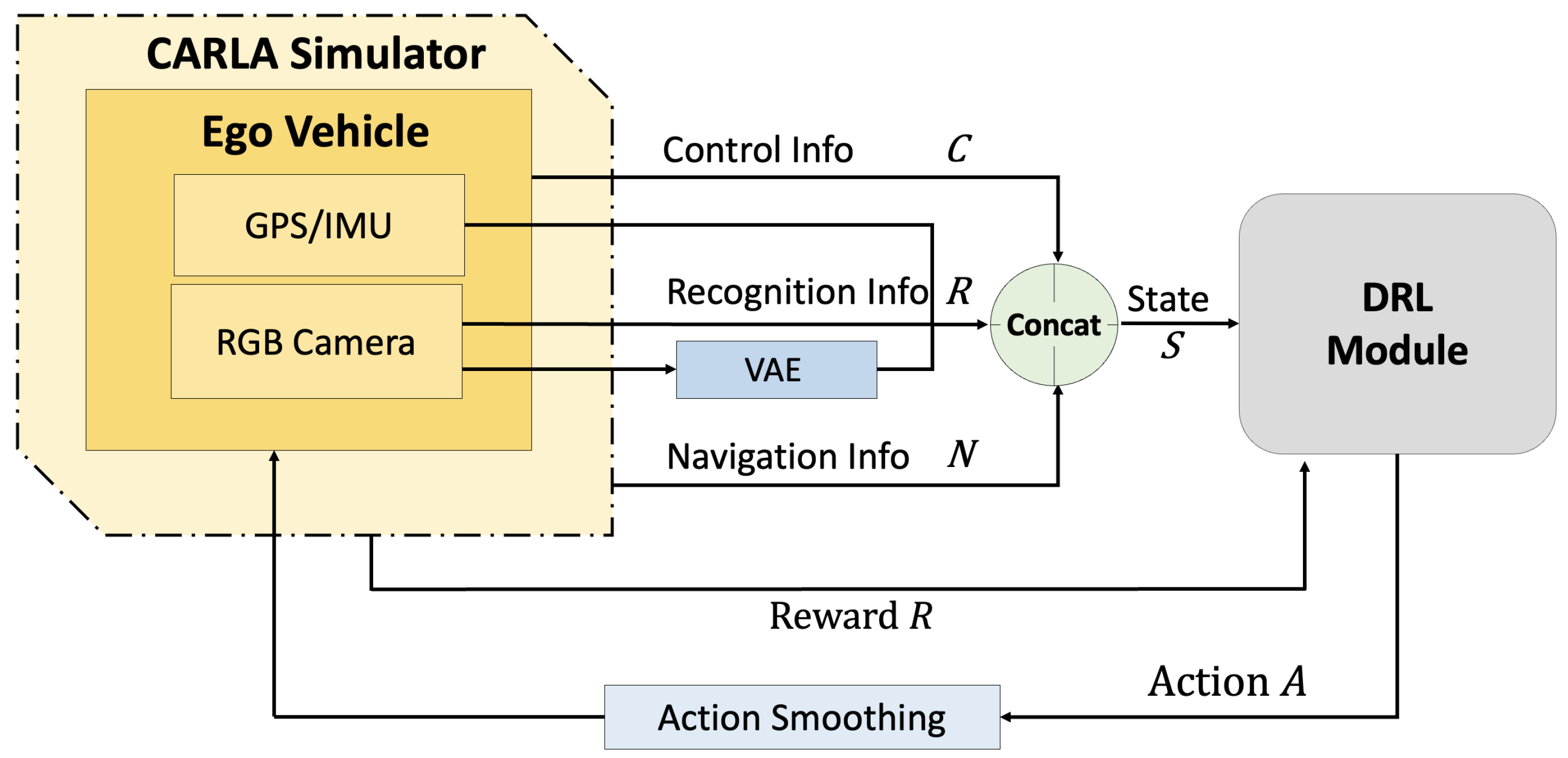

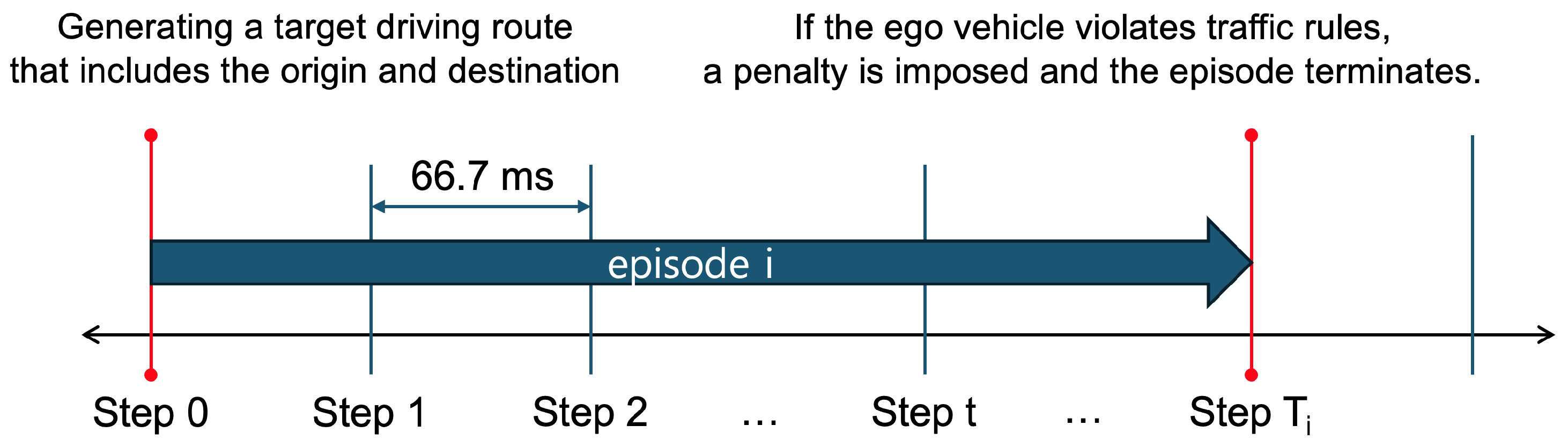
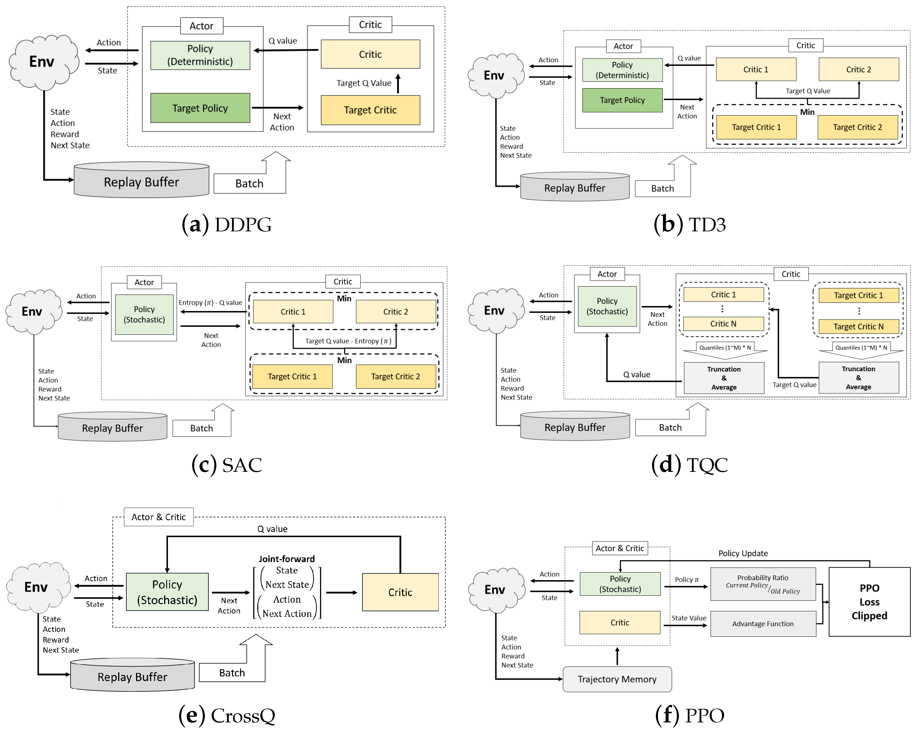
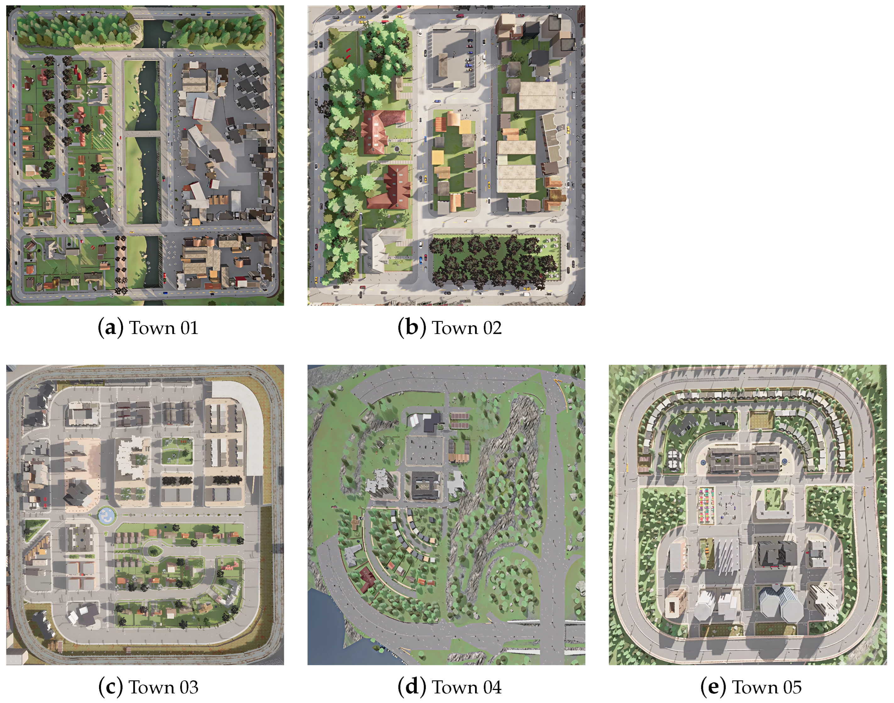
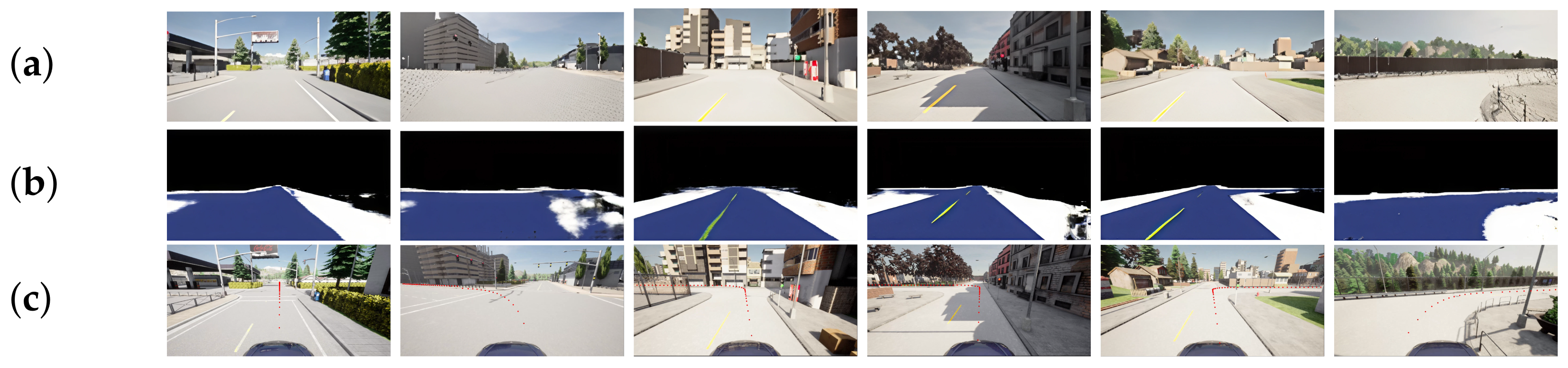
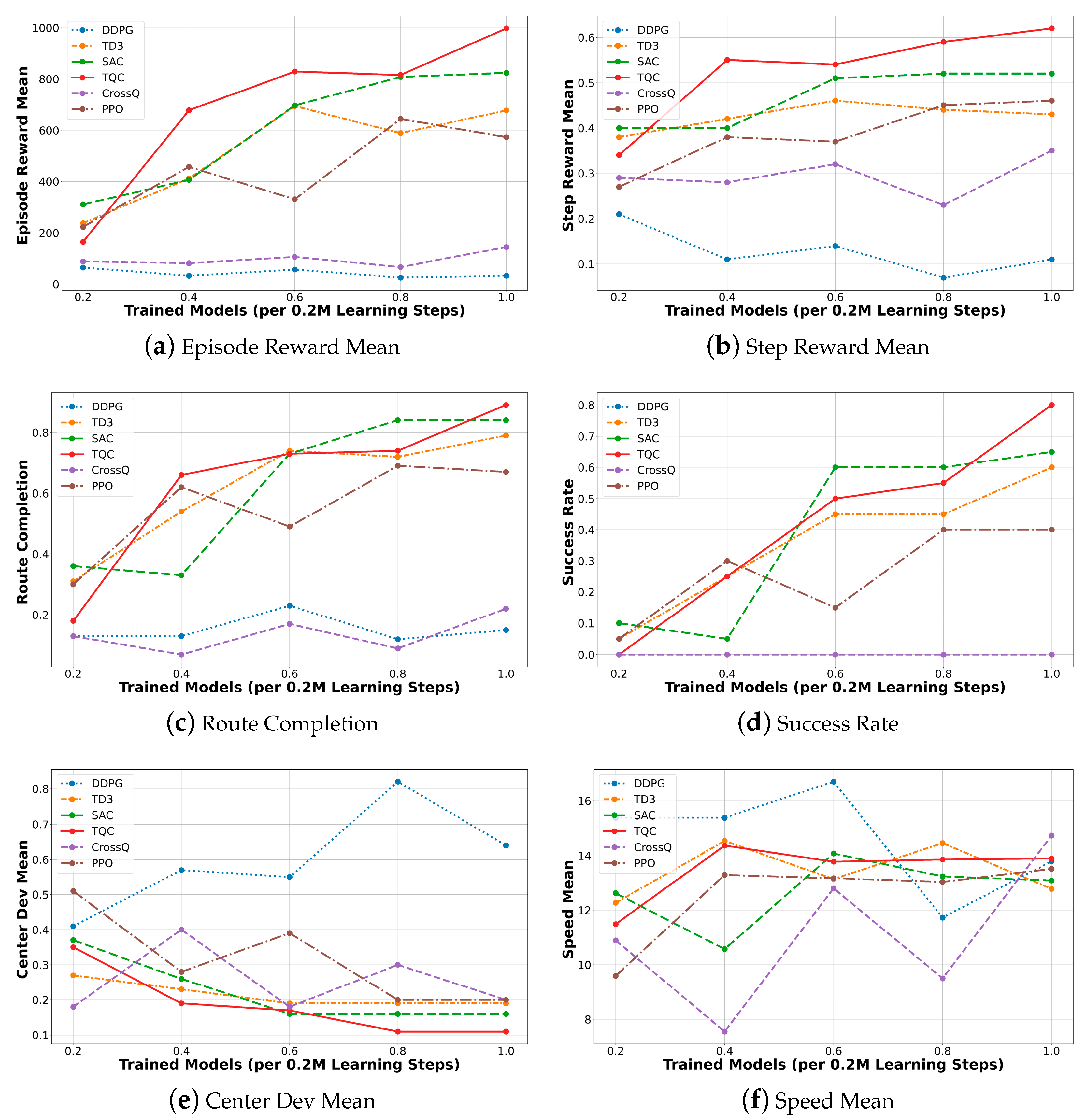
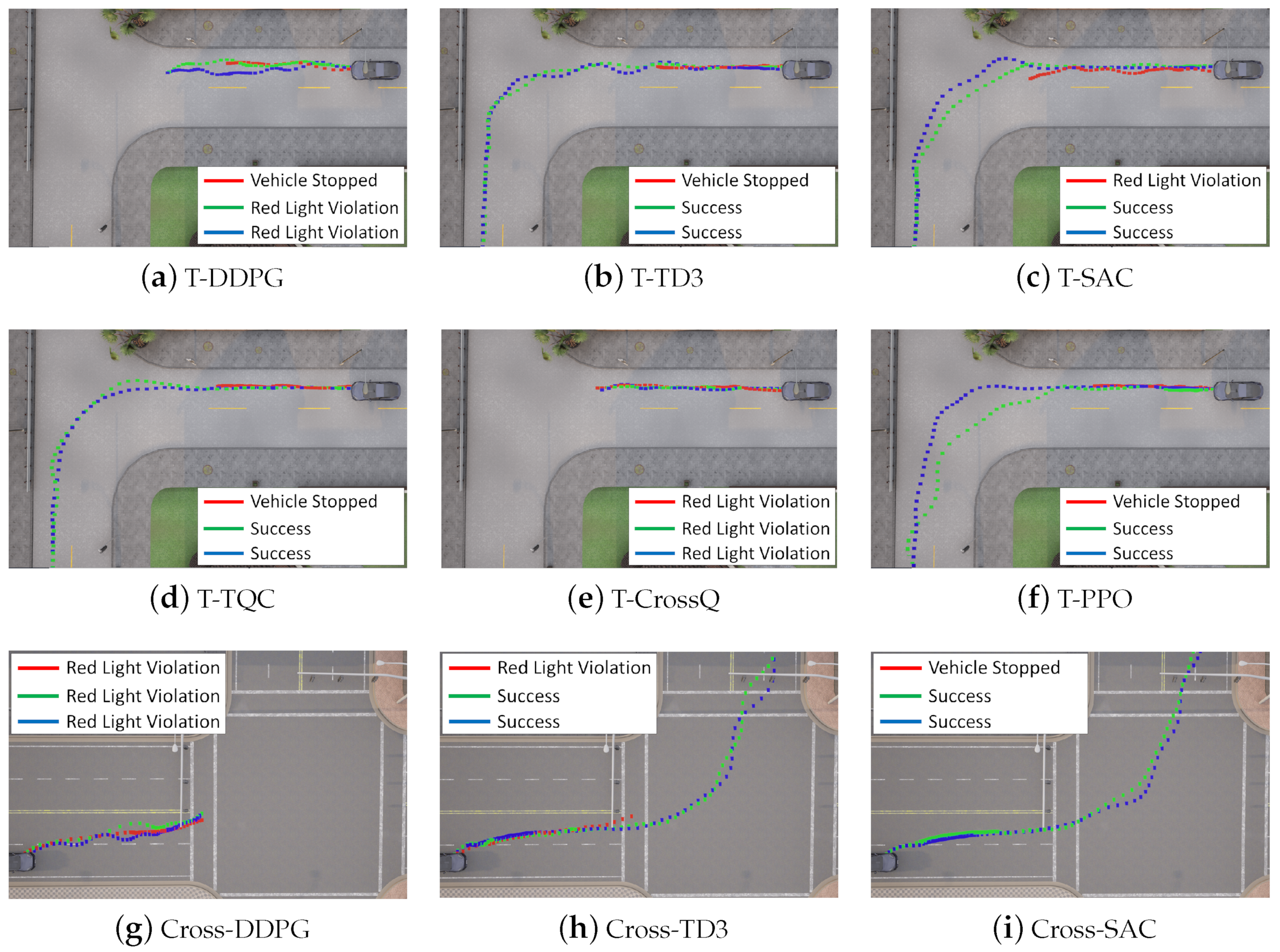
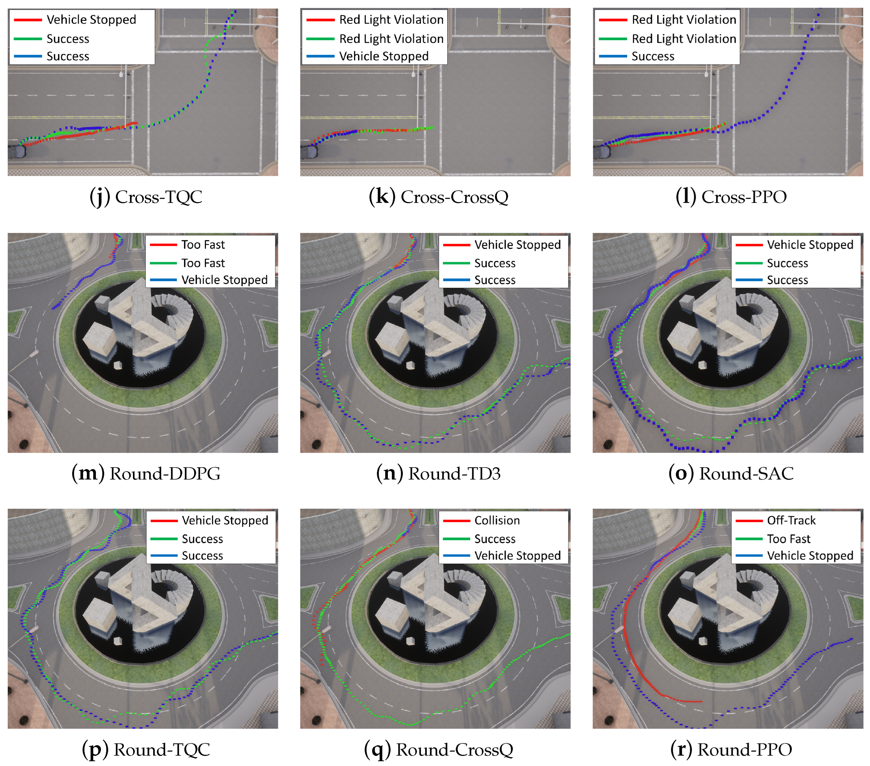
Disclaimer/Publisher’s Note: The statements, opinions and data contained in all publications are solely those of the individual author(s) and contributor(s) and not of MDPI and/or the editor(s). MDPI and/or the editor(s) disclaim responsibility for any injury to people or property resulting from any ideas, methods, instructions or products referred to in the content. |
© 2025 by the authors. Licensee MDPI, Basel, Switzerland. This article is an open access article distributed under the terms and conditions of the Creative Commons Attribution (CC BY) license (https://creativecommons.org/licenses/by/4.0/).