Simulation-Based Assessment of Urban Pollution in Almaty: Influence of Meteorological and Environmental Parameters

Abstract

Background: Air pollution is a persistent and critical challenge for Almaty, Kazakhstan’s largest city. The city’s unique topographical and meteorological conditions—being located in a mountain basin with dense urban development—restrict natural ventilation and contribute to frequent exceedances of air quality standards. These factors make accurate assessment and management of atmospheric pollution particularly urgent for the region. Aim: This study aims to develop and apply a novel, high-resolution three-dimensional numerical model to analyze the spatial distribution of key atmospheric indicators—air velocity, temperature, and pollutant concentrations in Almaty. The goal is to provide a comprehensive understanding of how meteorological and urban factors influence air quality, with a focus on both horizontal and vertical stratification. Methods: A three-dimensional computational model was constructed, integrating real meteorological data and detailed urban topography. The model solves the compressible Navier–Stokes, energy, and pollutant transport equations using the finite volume method over a 1000 × 1000 × 500 m domain. Meteorological fields are synthesized along all spatial axes to account for vortex structures, urban heat islands, and stratification effects. This approach enables the simulation of atmospheric parameters with unprecedented spatial resolution for Almaty. Results: The simulation reveals significant spatial heterogeneity in atmospheric parameters. Wind velocity ranges from 0.31 to 5.76 m/s (mean: 2.14 m/s), temperature varies between 12.03 °C and 19.47 °C (mean: 16.12 °C), and pollutant concentrations fluctuate from 5.02 to 102.35 μg/m³ (mean: 44.87 μg/m³). Notably, pollutant levels in the city center exceed those at the periphery by more than two-fold (68.23 μg/m³, 29.14 μg/m³), and vertical stratification leads to a marked decrease in concentrations with altitude. These findings provide, for the first time, a comprehensive and quantitative picture of air quality dynamics in Almaty. Conclusion: The developed model advances the scientific understanding of urban air pollution in complex terrains and offers practical tools for city planners and policymakers. By identifying pollution hotspots and elucidating the influence of meteorological factors, the model supports the optimization of urban infrastructure, zoning, and environmental monitoring systems. This research lays the groundwork for evidence-based strategies to mitigate air pollution and improve public health in Almaty and similar urban environments.

1. Introduction

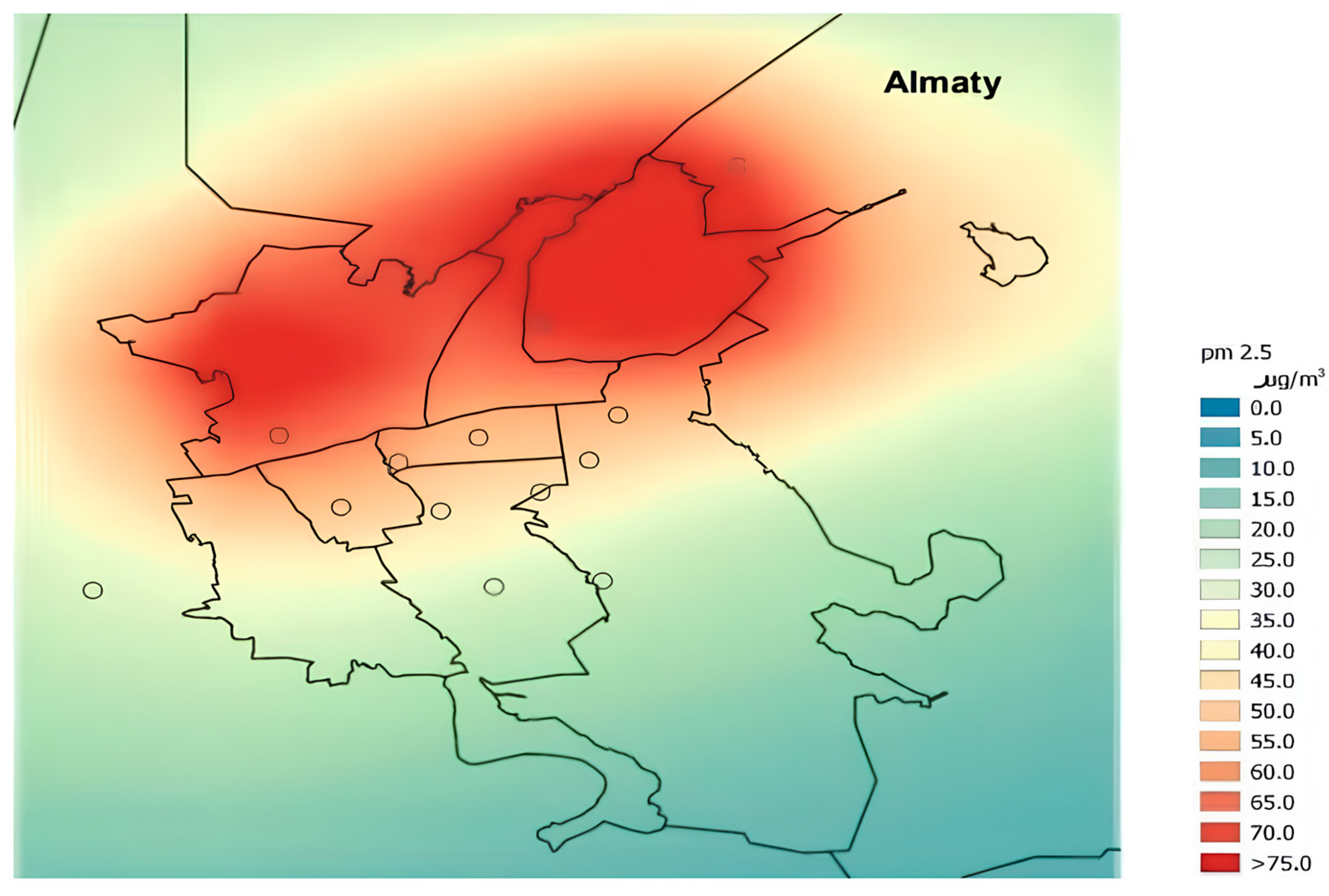
Almaty is the largest megacity of Kazakhstan, which annually ranks among the cities with the highest level of air pollution (see Figure 1) in the region. The geographical location in the foothill basin and high density of buildings contribute to the accumulation of harmful impurities, which is confirmed by monitoring data: average annual concentrations of PM_2.5 and NO₂ exceed WHO permissible standards 2–3 times (see Figure 2). In 2024, the number of days with clean air when the daily average PM_2.5 concentration remained within the WHO guidelines (daily average of 15 µg/m³) increased compared to 2023. While in 2023 there were only 137 such days, in 2024 there were 164.

Existing air quality assessment methods are mainly based on two-dimensional models or point measurements, which do not allow taking into account the complex structure of air flows and vertical stratification of pollutants. As a result, it is not possible to accurately predict and effectively manage air quality.

In this work, for the first time for Almaty, three-dimensional numerical modelling of pollutant distribution with regard to real meteorological and topographical conditions has been implemented. This makes it possible to identify spatial patterns of pollution distribution and propose new approaches to air quality monitoring and management.

Traditional methods of air quality monitoring, which rely on fixed, high-end monitoring stations, offer accurate measurements but are limited by their high deployment and maintenance costs, leading to sparse spatial coverage and the need for interpolation models to estimate air quality in unsampled areas [1]. An effective method for evaluating the environmental safety of urban areas involves analyzing the risks posed by various environmental pollution factors, providing a basis for environmental and sanitary measures to protect the population [2]. Advancements in artificial intelligence, particularly artificial neural networks, have ushered in new possibilities for tackling air quality and climate change-related problems, offering solutions to address the rising concerns about air pollution and its effects on human health and the environment [3,4]. This has led to the development of data-driven models that leverage big data from sources like traffic management and air pollutant concentration monitoring systems, enabling better urban planning, traffic route optimization, and the formulation of policies to mitigate carbon footprints [4]. These models, including machine learning algorithms, can predict air pollution levels across a city with high spatial and temporal resolution, addressing the limitations of traditional methods [5].

One promising avenue involves integrating meteorological and environmental parameters through sophisticated modeling techniques that can offer a more holistic understanding of pollution dynamics in Almaty. Conventional «bottom-up» models, such as Computational Fluid Dynamic Models, Chemical Transport Models, and CMAQ models, offer high model fidelity pertaining to the physical and chemical processes of air pollution [6]. However, these models necessitate detailed, high-resolution data on pollutant sources, topography, and meteorological conditions, which can be difficult and expensive to acquire for a city like Almaty. Statistical approaches, including machine learning methods like adaptive boosting, random forests, and support vector machines, have shown promising results in air quality index level predictions, using long-term datasets to account for seasonal and other factors [7]. These data-driven approaches can forecast air pollution levels, assisting authorities in implementing timely measures when high pollutant concentrations are expected [8]. Furthermore, the hybrid models that combine deterministic and statistical techniques can leverage the strengths of both approaches, potentially offering more accurate and reliable pollution assessments and predictions [9].

Although several studies have used CFD, CMAQ, or AI-based models for urban air pollution assessment [6,7,8,9], few integrate real-time meteorological data with high-resolution three-dimensional modeling tailored to a complex mountainous urban basin like Almaty. For instance, CMAQ models often simplify topography and focus on horizontal dispersion. Deep learning models such as Deep-AIR and Deep-MAPS provide temporal predictions but lack spatial resolution and physical interpretability.

Our study is the first to apply a fully three-dimensional, physically grounded CFD model with Navier–Stokes-based pollutant transport over a finely meshed urban domain for Almaty, incorporating real meteorological measurements, urban morphology, and vertical pollution stratification. This offers a new level of detail and accuracy for local environmental planning.

The deployment of low-cost sensor networks offers the potential to enhance the spatial resolution of air quality monitoring in Almaty. Despite their lower accuracy compared to reference-grade instruments, when properly calibrated and validated, these sensors can provide valuable data for identifying pollution hotspots and tracking pollution plumes [10]. This data, when combined with meteorological data such as wind speed, wind direction, temperature, and humidity, can help elucidate the transport and dispersion patterns of pollutants. These networks, along with weather data and particulate matter readings, can be used to train Long Short-Term Memory models to forecast and classify air quality, which has been shown to significantly reduce pollution in urban environments. The integration of data from various sources, including satellite remote sensing, ground-based monitoring stations, and meteorological models, can provide a comprehensive view of air quality and its relationship with meteorological conditions.

The intricate interplay between meteorological factors and pollution levels underscores the necessity for sophisticated analytical approaches, where advancements in machine learning offer a potent tool for unraveling these complex relationships and developing predictive models that can inform effective pollution control strategies in Almaty [7,11]. Deep learning models, particularly those employing Convolutional LSTM-SDAE architectures, can effectively model temporal dependencies and correlations between pollutants and meteorological factors, improving prediction accuracy by addressing issues such as missing data [12]. One can employ deep learning models to develop air quality forecasting and classification systems by training LSTM models on sensor data, meteorology, aerosol optical depth, and particulate matter readings [13]. Furthermore, satellite data, with its global availability and frequent updates, can be integrated with deep learning models to estimate air pollution, even in areas with limited ground-based monitoring [14]. By fusing satellite information with pollution measurements, even simpler models can work effectively, allowing for accurate air quality predictions, which is applicable to locations where monitoring stations do not exist [10].

Mobile air pollution sensing, enhanced by machine learning frameworks, presents a cost-effective approach to obtain high-resolution air quality information across the city, even with sparse sensing coverage. By leveraging urban big data, these frameworks can generate insights into the potential causes of pollution, supporting evidence-based sustainable urban management [6]. The integration of remote sensing data with machine learning techniques enables the estimation of air pollution at high spatial resolution, adding a temporal dimension to these estimates [10,14]. The use of ensemble learning algorithms, such as XGBoost, support vector machines, and generalized additive models, to establish regression models based on environmental monitoring data, including meteorological factors and pollution levels, can provide timely warnings of respiratory disease risks [15]. Furthermore, understanding the relationship between air pollution and mortality and developing predictive models for respiratory disease-related deaths due to air pollution is critical for protecting vulnerable populations.

A thorough environmental assessment is required to diminish contamination within a catchment scale [16]. Such a comprehensive strategy should incorporate the complexities of hydrological, economic, and ecological elements [17]. An integrated approach must consider the intricate web of interactions between environmental, social, and economic factors, recognizing that pollution does not exist in isolation but rather as a symptom of broader systemic issues [18]. This perspective acknowledges that effective pollution management requires addressing the root causes of environmental degradation, which often lie in unsustainable consumption patterns, inadequate regulatory frameworks, and inequitable distribution of resources.

Finally, the integration of traffic control technologies with artificial intelligence is a relevant research topic in urban ecology as well, which is also addressed in [19]. This paper proposes the use of Adaptive Neural Functional Inference Systems (ANFIS) to model and analyze vehicle emissions data and its impact on air quality. The results show that the combination of traffic management and AI technologies can effectively assess and improve air quality in urban areas.

The novelty of the study lies in the complex modeling of interrelated atmospheric fields (velocity, temperature, and concentration), taking into account specific urban factors; analysis of the vertical structure of parameter distribution at different altitudinal slices; quantitative assessment of the impact of urban heat islands and industrial zones on the distribution of pollutants; as well as in the development of a methodology for visualizing the results with accurate numerical characteristics, ensuring reproducibility and practical applicability for environmental.

The aim of the study is to develop and apply a numerical model to estimate the distribution of key atmospheric indicators, which are air velocity, temperature, and pollutant concentrations, in an urban environment considering different altitude slices.

2. Materials and Methods

2.1. Study Area

Almaty, Kazakhstan’s largest metropolis, grapples with significant air pollution challenges stemming from a confluence of factors including industrial emissions, vehicular traffic, and geographical constraints, necessitating a comprehensive and integrated approach to pollution assessment [20].

To describe the dynamics of pollutants in the atmosphere, a system of compressible Navier-Stokes equations is used, supplemented by an equation for the transport of pollutants with dispersion and reaction components. Continuity equation (conservation of mass):

$${\displaystyle \frac{\partial \rho }{\partial t}}+{\displaystyle \frac{\partial \left(\rho u\right)}{\partial x}}+{\displaystyle \frac{\partial \left(\rho v\right)}{\partial x}}+{\displaystyle \frac{\partial \left(\rho w\right)}{\partial x}}=0$$

(1)

here $\rho$ is density, $t$ is time, $x$, $y$, $z$ are coordinates in space, $u$, $v$, $w$ are components of velocities.

Equations of conservation of momentum:

$${\displaystyle \frac{\partial \left(\rho u\right)}{\partial t}}+{\displaystyle \frac{\partial \left(\rho u^2\right)}{\partial x}}+{\displaystyle \frac{\partial \left(\rho uv\right)}{\partial y}}+{\displaystyle \frac{\partial \left(\rho uw\right)}{\partial z}}=-{\displaystyle \frac{\partial P}{\partial x}}+{\displaystyle \frac{\partial {\tau }_{xx}}{\partial x}}+{\displaystyle \frac{\partial {\tau }_{xy}}{\partial y}}+{\displaystyle \frac{\partial {\tau }_{xz}}{\partial z}}+\rho f_x,$$

$${\displaystyle \frac{\partial \left(\rho v\right)}{\partial t}}+{\displaystyle \frac{\partial \left(\rho uv\right)}{\partial x}}+{\displaystyle \frac{\partial \left(\rho v^2\right)}{\partial y}}+{\displaystyle \frac{\partial \left(\rho vw\right)}{\partial z}}=-{\displaystyle \frac{\partial P}{\partial y}}+{\displaystyle \frac{\partial {\tau }_{xy}}{\partial x}}+{\displaystyle \frac{\partial {\tau }_{yy}}{\partial y}}+{\displaystyle \frac{\partial {\tau }_{yz}}{\partial z}}+\rho f_y,$$

(2)

$${\displaystyle \frac{\partial \left(\rho w\right)}{\partial t}}+{\displaystyle \frac{\partial \left(\rho uw\right)}{\partial x}}+{\displaystyle \frac{\partial \left(\rho vw\right)}{\partial y}}+{\displaystyle \frac{\partial \left(\rho w^2\right)}{\partial z}}=-{\displaystyle \frac{\partial P}{\partial z}}+{\displaystyle \frac{\partial {\tau }_{xz}}{\partial x}}+{\displaystyle \frac{\partial {\tau }_{yz}}{\partial y}}+{\displaystyle \frac{\partial {\tau }_{zz}}{\partial z}}+\rho f_z,$$

where $f_x$, $f_y$, $f_z$ are external forces, the components of the viscous stress tensor for a Newtonian fluid are:

$${\tau }_{xx}=\mu \left(2{\displaystyle \frac{\partial u}{\partial x}}-{\displaystyle \frac{2}{3}}\nabla ·\overrightarrow{u}\right), {\tau }_{yy}=\mu \left(2{\displaystyle \frac{\partial v}{\partial y}}-{\displaystyle \frac{2}{3}}\nabla ·\overrightarrow{u}\right), {\tau }_{zz}=\mu \left(2{\displaystyle \frac{\partial w}{\partial z}}-{\displaystyle \frac{2}{3}}\nabla ·\overrightarrow{u}\right),$$

$${\tau }_{xy}={\tau }_{yx}=\mu \left({\displaystyle \frac{\partial u}{\partial y}}+{\displaystyle \frac{\partial v}{\partial x}}\right), {\tau }_{xz}={\tau }_{zx}=\mu \left({\displaystyle \frac{\partial u}{\partial z}}+{\displaystyle \frac{\partial w}{\partial x}}\right), {\tau }_{yz}={\tau }_{zy}=\mu \left({\displaystyle \frac{\partial v}{\partial z}}+{\displaystyle \frac{\partial w}{\partial y}}\right)$$

Energy conservation equation:

$${\displaystyle \frac{\partial \left(\rho E\right)}{\partial t}}+{\displaystyle \frac{\partial \left(\rho uE+up\right)}{\partial x}}+{\displaystyle \frac{\partial \left(\rho vE+vp\right)}{\partial y}}+{\displaystyle \frac{\partial \left(\rho wE+wp\right)}{\partial z}}={\displaystyle \frac{\partial }{\partial x}}\left(k{\displaystyle \frac{\partial T}{\partial x}}\right)+{\displaystyle \frac{\partial }{\partial y}}\left(k{\displaystyle \frac{\partial T}{\partial y}}\right)+{\displaystyle \frac{\partial }{\partial z}}\left(k{\displaystyle \frac{\partial T}{\partial z}}\right)+\Phi +Q,$$

(3)

$E=e+{\displaystyle \frac{1}{2}}\left(u^2+v^2+w^2\right)$ is total energy per unit mass, $e$ is internal energy per unit mass, $k$ is thermal conductivity coefficient, $\Phi$ is dissipation function (conversion of kinetic energy into thermal energy due to viscosity), $Q$ is external heat sources.

For air, the ideal gas equation can be used:

$$P=\rho RT,$$

(4)

where R is the gas constant for air.

Temperature equation:

$${\displaystyle \frac{\partial \left(\rho T\right)}{\partial t}}+{\displaystyle \frac{\partial \left(\rho uT\right)}{\partial x}}+{\displaystyle \frac{\partial \left(\rho vT\right)}{\partial y}}+{\displaystyle \frac{\partial \left(\rho wT\right)}{\partial z}}={\displaystyle \frac{\partial }{\partial x}}\left(D{\displaystyle \frac{\partial T}{\partial x}}\right)+{\displaystyle \frac{\partial }{\partial y}}\left(D{\displaystyle \frac{\partial T}{\partial y}}\right)+{\displaystyle \frac{\partial }{\partial z}}\left(D{\displaystyle \frac{\partial T}{\partial z}}\right),$$

(5)

where T is the temperature. The equation for the transfer of pollutant concentrations:

$${\displaystyle \frac{\partial \left(\rho C\right)}{\partial t}}+{\displaystyle \frac{\partial \left(\rho uC\right)}{\partial x}}+{\displaystyle \frac{\partial \left(\rho vC\right)}{\partial y}}+{\displaystyle \frac{\partial \left(\rho wC\right)}{\partial z}}={\displaystyle \frac{\partial }{\partial x}}\left(D{\displaystyle \frac{\partial C}{\partial x}}\right)+{\displaystyle \frac{\partial }{\partial y}}\left(D{\displaystyle \frac{\partial C}{\partial y}}\right)+{\displaystyle \frac{\partial }{\partial z}}\left(D{\displaystyle \frac{\partial C}{\partial z}}\right)+S,$$

(6)

where C is the mass concentration of the pollutant, D is the diffusion coefficient of the pollutant, S is the sources of the pollutant.

For a simplified model, all equations can be reduced to a combined numerical scheme, where the Navier-Stokes equations interact to model the movement of the air mass and the effect of wind, the temperature equation takes into account the effect of temperature gradients on the density and speed of air, and the concentration equation models the attenuation, diffusion, and transport of pollutants along with the air flow. This combined model allows the use of meteorological parameters (wind speed, temperature, and pressure) to calculate the velocity vector, temperature, and concentration.

2.2. Initial and Boundary Conditions

Initial conditions ($t=0$) for air density: $\rho \left(x,y,z,0\right)={\rho }_0\left(x,y,z\right)$. For the city of Almaty, you can use the barometric formula, taking into account the altitude above sea level:

$${\rho }_0\left(x,y,z\right)={\rho }_{sea}exp\left(-{\displaystyle \frac{g\left(z+h_{Almaty}\right)}{R{T}_0}}\right),$$

where $h_{Almaty}\approx 800$ m is the average height of Almaty above sea level.

Velocity components are:

$$u\left(x,y,z,0\right)=u_0\left(x,y,z\right),$$

$$v\left(x,y,z,0\right)=v_0\left(x,y,z\right),$$

$$w\left(x,y,z,0\right)=w_0\left(x,y,z\right).$$

Temperature is $T\left(x,y,z,0\right)=T_0\left(x,y,z\right)$. Almaty is characterized by a temperature gradient by height, as well as a temperature inversion in winter:

$$T_0\left(x,y,z\right)=T_{surface}-\gamma z,$$

where γ is the vertical temperature gradient.

Pressure is $P\left(x,y,z,0\right)=P_0\left(x,y,z\right)$. The initial pressure distribution can be specified in the hydrostatic approximation:

$$P_0\left(x,y,z\right)=P_{surface}exp\left(-{\displaystyle \frac{g\left(z\right)}{R{T}_0\left(z\right)}}\right).$$

Concentration of pollutants:

$$C\left(x,y,z,0\right)=C_0\left(x,y,z\right).$$

The calculation domain is a parallelepiped $\Omega =\left[0,L_x\right]\times \left[0,L_y\right]\times \left[0,L_z\right]$, where $L_x$, $L_y$, $L_z$ are the dimensions of the domain in the corresponding directions.

Boundary conditions at the lower boundary (ground, $z=0$):

For the velocity, the no-slip condition $u\left(x,y,0,t\right)=0$, $v\left(x,y,0,t\right)=0$, $w\left(x,y,0,t\right)=0$ are used.

For the temperature of the earth, the surface temperature will be $T\left(x,y,0,t\right)=T_{surface}\left(x,y,t\right)$.

For the concentration at $z=0$, there will be a given flow of pollutants $-D{\displaystyle \frac{\partial C}{\partial z}}\left(x,y,0,t\right)=q_C\left(x,y,t\right)$, where $q_C$ is the intensity of the emission of pollutants from the surface.

For the velocity at the upper boundary ($z=L_z$) the free exit condition is set

$${\displaystyle \frac{\partial u}{\partial z}}\left(x,y,L_z,t\right)=0, {\displaystyle \frac{\partial v}{\partial z}}\left(x,y,L_z,t\right)=0, {\displaystyle \frac{\partial w}{\partial z}}\left(x,y,L_z,t\right)=0.$$

For the temperature at the upper boundary ($z=L_z$) the temperature gradient is specified:

$${\displaystyle \frac{\partial T}{\partial z}}\left(x,y,L_z,t\right)=-{\gamma }_{atm},$$

where ${\gamma }_{atm}$ is the adiabatic temperature gradient in the atmosphere.

For the concentration at the upper boundary ($z=L_z$), the free exit condition is set:

$${\displaystyle \frac{\partial C}{\partial z}}\left(x,y,L_z,t\right)=0.$$

At the lateral boundaries, periodic boundary conditions or flow entry/exit conditions, depending on the wind direction, can be used. At the inlet boundary (for $u>0$ at $x=0$):

$$u\left(0,y,z,t\right)=u_{in}\left(y,z,t\right), v\left(0,y,z,t\right)=v_{in}\left(y,z,t\right), w\left(0,y,z,t\right)=w_{in}\left(y,z,t\right),$$

$$T\left(0,y,z,t\right)=T_{in}\left(y,z,t\right), C\left(0,y,z,t\right)=C_{in}\left(y,z,t\right).$$

At the output boundary (for $u>0$ at $x=L_x$):

$${\displaystyle \frac{\partial u}{\partial x}}\left(L_x,y,z,t\right)=0, {\displaystyle \frac{\partial v}{\partial x}}\left(L_x,y,z,t\right)=0, {\displaystyle \frac{\partial w}{\partial x}}\left(L_x,y,z,t\right)=0,$$

$${\displaystyle \frac{\partial T}{\partial x}}\left(L_x,y,z,t\right)=0, {\displaystyle \frac{\partial C}{\partial x}}\left(L_x,y,z,t\right)=0.$$

The values of the initial and boundary conditions—such as air temperature at the surface, pollutant concentration, wind velocity, pressure, and vertical temperature gradient—were determined based on the averaged historical data provided by the Kazakh Hydrometeorological Service (Kazhydromet) for the period 2015–2024.

The vertical temperature gradient (γ) was set according to observed inversion profiles in winter and adiabatic lapse rates during summer months, as derived from balloon sounding data at the Almaty meteorological station. The initial surface temperature of T₀ = 17 °C corresponds to the seasonal mean for early spring months, based on long-term climatic data.

The pollutant concentration at ground level (C₀ = 0.8 g/m³) reflects average daily concentrations of PM_2.5 and PM₁₀ during episodes of high pollution recorded in central Almaty, as reported by Kazhydromet bulletins.

Wind speed values at inlet boundaries were calibrated using monthly average wind roses and adjusted for altitude and urban roughness effects via barometric and logarithmic vertical wind profiles.

These sources ensure that the model is grounded in real-world measurements and remains consistent with climatological and environmental norms for the city.

2.3. Numerical Solution Methodology

The Finite Volume Method (FVM) is used to solve the system of compressible Navier-Stokes equations with temperature and pollutant concentration equations.

We divide the calculation area into cells of size $∆x\times ∆y\times ∆z$. The cell centers have coordinates:

$$x_i=\left(i-0.5\right)∆x, i=1,2,\dots ,N_x$$

$$y_j=\left(i-0.5\right)∆y, j=1,2,\dots ,N_j$$

$$z_k=\left(i-0.5\right)∆z. k=1,2,\dots ,N_z$$

We use an explicit scheme of the first order of accuracy (Euler’s scheme):

$${\displaystyle \frac{{\varphi }^{n+1}-{\varphi }^n}{∆t}}=RHS\left({\varphi }^n\right),$$

where ${\varphi }^n$ is any of the desired variables $\left(\rho ,u,v,w,T,C\right)$, and $RHS\left({\varphi }^n\right)$ is the right-hand side of the corresponding equation.

The continuity Equation (1) for discretization has the form

$${\displaystyle \frac{{\rho }_{i,j,k}^{n+1}-{\rho }_{i,j,k}^n}{∆t}}+{\displaystyle \frac{{\left(\rho u\right)}_{i+1/2,j,k}^n-{\left(\rho u\right)}_{i-1/2,j,k}^n}{∆x}}+{\displaystyle \frac{{\left(\rho v\right)}_{i,j+1/2,k}^n-{\left(\rho v\right)}_{i,j-1/2,k}^n}{∆y}}+{\displaystyle \frac{{\left(\rho w\right)}_{i,j,k+1/2}^n-{\left(\rho w\right)}_{i,j,k-1/2}^n}{∆z}}=0.$$

The discretized form of the momentum Equation (2) for the component u is:

$$\begin{array}{c}{\left(\rho u\right)}_{i,j,k}^{n+1}={\left(\rho u\right)}_{i,j,k}^n-∆t\left[{\displaystyle \frac{{\left(\rho u^2\right)}_{i+\frac{1}{2},j,k}^n-{\left(\rho u^2\right)}_{i-\frac{1}{2},j,k}^n}{∆x}}+{\displaystyle \frac{{\left(\rho uv\right)}_{i,j+\frac{1}{2},k}^n-{\left(\rho uv\right)}_{i,j-\frac{1}{2},k}^n}{∆y}}+{\displaystyle \frac{{\left(\rho uw\right)}_{i,j,k+\frac{1}{2}}^n-{\left(\rho uw\right)}_{i,j,k-\frac{1}{2}}^n}{∆z}}\right]\\ \hspace{1em}\hspace{1em}\hspace{1em}\hspace{1em}\hspace{1em} -∆t{\displaystyle \frac{P_{i+\frac{1}{2},j,k}^n-P_{i-\frac{1}{2},j,k}^n}{2∆x}}+∆t{\left[\mathrm{d}\mathrm{i}\mathrm{f}\mathrm{f}\mathrm{u}\mathrm{s}\mathrm{i}\mathrm{o}\mathrm{n} \mathrm{t}\mathrm{e}\mathrm{r}\mathrm{m}\mathrm{s}\right]}_{jk}^n+∆t{\left[\rho f_x\right]}_{jk}^n\end{array}$$

Similar equations can be written for the velocity components v and w along the y and z axes, respectively.

The discretization of the energy (3) temperature (5) equations is performed similarly.

The concentration Equation (6) is given in the following form:

$${\displaystyle \frac{{\left(\rho C\right)}_{i,j,k}^{n+1}-{\left(\rho C\right)}_{i,j,k}^n}{∆t}}+\left[\mathrm{c}\mathrm{o}\mathrm{n}\mathrm{v}\mathrm{e}\mathrm{c}\mathrm{t}\mathrm{i}\mathrm{v}\mathrm{e} \mathrm{m}\mathrm{e}\mathrm{m}\mathrm{b}\mathrm{e}\mathrm{r}\mathrm{s}\right]=\left[\mathrm{d}\mathrm{i}\mathrm{f}\mathrm{f}\mathrm{u}\mathrm{s}\mathrm{i}\mathrm{o}\mathrm{n} \mathrm{t}\mathrm{e}\mathrm{r}\mathrm{m}\mathrm{s}\right]+S_{i,j,k}^n.$$

For an explicit scheme, the Courant-Friedrichs-Lewy ($CFL$) condition must be met:

$$∆t\le min\left({\displaystyle \frac{∆x}{\left|u\right|+c}},{\displaystyle \frac{∆y}{\left|v\right|+c}},{\displaystyle \frac{∆z}{\left|w\right|+c}}\right)·CFL,$$

where $c$ is the speed of sound, and $CFL$ is the Courant number ($CFL<1$).

The model uses a structured grid with spatial resolution of 10 × 10 × 10 m³ per cell in a domain of 1000 × 1000 × 500 m, resulting in a total of 5 million grid cells. Such a high spatial resolution allows detailed resolution of urban-scale features such as building-induced wind shear, urban heat islands, and pollutant trapping in street canyons.

The temporal resolution is set to 1 s, ensuring compliance with the Courant–Friedrichs–Lewy (CFL) condition for numerical stability (CFL < 1). This fine temporal resolution permits accurate simulation of fast-changing atmospheric processes, including eddy formation and short-term wind speed fluctuations.

Compared to coarser models (e.g., with cell sizes of 100 m or greater), our high-resolution scheme significantly enhances the ability to detect micro-scale airflow variations and pollutant stratification, which are critical for cities like Almaty with highly variable topography and meteorological inversion layers.

The model’s robustness was confirmed through sensitivity analysis of Peclet numbers, indicating dominant advection with balanced diffusion behavior. This configuration minimizes numerical dispersion and ensures physical fidelity of the computed fields.

2.4. Statistical Analysis

To interpret the simulation results, we applied basic descriptive statistical tools to analyze spatial and vertical distributions of wind velocity, temperature, and pollutant concentrations. For each atmospheric parameter, the following indicators were computed: mean value over the entire computational domain and specific altitude slices; maximum and minimum values to identify pollution hotspots and ventilation zones; standard deviation to assess spatial heterogeneity and dynamic variation; vertical concentration gradients, defined as

$$C_z={\displaystyle \frac{C_{z=0}-C_{z=h}}{h}},$$

where $C_z$ is the pollutant concentration at altitude $z$, and $h$ is the height difference.

2.5. Model Limitations and Practical Implications

The developed model offers a powerful tool for practical applications such as zoning recommendations, urban ventilation planning, and pollution sensor placement in cities with complex topography like Almaty.

However, the model has several limitations: it does not incorporate chemical transformation of pollutants, uses a simplified turbulence scheme, and is limited to a single-hour simulation window.

Future improvements may include coupling with chemical transport models, real-time sensor feedback loops, and adaptive meshing for localized emission zones. Despite these limitations, the current model remains highly informative for evidence-based urban environmental planning.

The use of the full compressible Navier–Stokes equations, while computationally intensive, allows for accurate modeling of airflow in a complex urban environment. Although small-scale turbulence is not explicitly resolved (as would be done with LES), the large-scale convective and diffusive transport processes are adequately captured due to the fine spatial grid and physically justified boundary conditions.

This approach is suitable for mesoscale urban applications, such as identifying ventilation corridors, stratification effects, and pollutant accumulation zones. Future research could explore coupling the current model with turbulence closure schemes (e.g., k–ε or LES) to enhance resolution in street-canyon scale flows.

3. Results

For numerical simulation, the parameters from

Table 1. Simulation parameters.

Description	Value
Area dimensions, $L_x\times L_y\times L_z$	1000 × 1000 × 500 m
Computational grid sizes, $N_x\times N_y\times N_z$	100 × 100 × 50
Step in $x$ direction, $∆x$	25 m
Step in $y$ direction, $∆y$	25 m
Step in $z$ direction, $∆z$	20 m
Time step $t$, $∆t$	1 s
Total simulation time	3600 s (1 h)
Diffusion coefficient for contamination	5.0 m2/s
Diffusion coefficient for temperature	2.0 m2/s
Maximum speed (advection)	4.0 m/s
Peclet number for contamination	by x 800, by z 400
Peclet number for temperature	by x 2000, by z 1000
Stability condition	CFL < 1

were used.

Figure 3 shows the wind speed field at ground level (z = 0 m). Approximately, the average speed along the u-axis is about 5.43 m/s (average value over the entire area), maximum ≈ 7.80 m/s, and minimum ≈ 3.20 m/s; the resulting speed has an average value of about 5.50 m/s and a maximum of ≈ 9.25 m/s.

At ground level (z = 0 m), the air velocity (see Figure 3a) is characterized by comparatively low values: the average velocity is about 0.76 m/s, with the maximum value reaching 1.67 m/s. This is typical for the boundary layer, where the influence of surface friction is significant. At a height of 131.6 m (see Figure 3b), the average velocity increases to 1.66 m/s, which reflects the decrease in the influence of surface friction. At a height of 263.2 m (see Figure 3c), the average velocity reaches 2.24 m/s, and at a level of 500 m (see Figure 3d), it is already 3.01 m/s with a maximum value of up to 4.0 m/s.

The analysis presented in

Table 2. Wind velocity analysis.

Description	Value
Mean u-velocity	2.07 m/s
Max u-velocity	4 m/s
Min u-velocity	−0.33 m/s
Mean v-velocity	0 m/s
Max v-velocity	0.5 m/s
Min v-velocity	−0.5 m/s
Mean resultant speed	2.09 m/s
Max resultant speed	4 m/s

confirms the presence of velocity gradients in the horizontal plane, which is visible in the distribution of vectors in the velocity field graphs. The presence of zones with higher and lower velocity values may indicate local dynamic effects.

These values are summarized in Table 2,

Table 3. Analysis of temperature.

Time (s)	Mean Temperature (°C)	Maximum Temperature (°C)	Minimum Temperature (°C)
0	14.06	25	8
900	14.02	18.96	9.49
1800	14	18.12	9.96
2700	14	17.69	10.32
3600	14	17.38	10.63

and

Table 4. Analysis of concentration.

Time (s)	Mean Concentration (μg/m3)	Maximum Concentration (μg/m3)	Total Mass (μg/m3)
0	0.8	100	437,317,784.26
900	0.06	3.59	34,312,776.64
1800	0	0.59	2,588,394.67
2700	0	0.04	191,033.42
3600	0	0	14,043.06

, and further visualized in Figure 3, Figure 4, Figure 5 and Figure 6. The use of descriptive statistics enabled a quantifiable comparison across spatial dimensions and supported the identification of pollution accumulation patterns and stratification effects under real meteorological conditions.

The obtained data (see Table 2) demonstrate that the model adequately describes the dynamics of the wind flow: an increase in speed with height indicates a decrease in the effect of surface friction, and the horizontal distribution shows the distribution of air movement speed characteristic of the layer boundaries.

Figure 4 shows temperature profiles (in °C) for different altitude levels (approximately: z = 0 m, z ≈ 131.6 m, z ≈ 263.2 m, and z = 500 m). At ground level, the temperature has average values of about 17.37 °C, and at the upper boundary (z = 500 m) it is about 10.63 °C, which reflects the vertical temperature gradient.

Figure 4a shows a fairly uniform temperature distribution with a clear horizontal layer, where the average values are close to 17–17.38 °C. This indicates that at the initial level there is a relative isotropy of the heat distribution process after stabilization. At the altitude z = 131.6 m (see Figure 4b), the average temperature is slightly lower (about 16.35 °C). The graph shows a more pronounced gradient than at ground level, indicating an effective vertical decrease in temperature with increasing altitude. The temperature further decreases to 13.72 °C (see Figure 4c). The distribution shows that the influence of the surface weakens and the inversion of layers becomes noticeable—the heat distribution is more uniform, but with a general decrease in values. At the altitude z = 500 m, Figure 4d shows the lowest temperature values are about 10.63 °C. Here, a clear vertical gradient is observed, typical for the atmospheric distribution, where the upper layers are significantly cooled compared to the lower ones.

Figure 5 illustrates the distribution of pollution at ground level (in µg/m³). According to calculations, in the final time step, the average concentration was about 0 µg/m³ (with maximum local values close to zero, as the pollution gradually dissipated), and the total mass of pollutant for this slice was about 140.57 µg.

Figure 5a shows a significant concentration of pollution at the initial moment, but at the final state the concentrations are reduced to zero (the average value is almost 0 μg/m³), and the total mass for this section has significantly decreased. This indicates an effective dilution of the pollutant over the zone. At the height of z = 131.6 m, the concentration (see Figure 5b) also almost disappears, which confirms that the processes of dispersion and diffusion work effectively not only at ground level but also in the upper layers of the atmosphere. At the height of 263.2 m and at the height of 500 m, the concentration of pollution (Figure 5c,d) is almost zero. This indicates that even if the initial pollution was localized, as a result of dynamic processes (advection and diffusion), the substance was uniformly distributed, and its local concentration decreased to a level of almost zero.

Temperature and concentration analyses and simulation parameters are presented in Table 3 and Table 4.

The average, maximum, and minimum temperatures change little over time. The initial data show that at t = 0, the average temperature is 14.06 °C, the maximum is 25.0 °C, and the minimum is 8.0 °C. As the simulation progresses, the maximum and minimum values converge to approximately 14.0 °C, indicating that the temperature in the computational domain is leveling off.

At the start of the simulation, the concentration of pollution is quite high (average value 0.8 μg/m³, maximum 100 μg/m³) and the total mass of the pollutant is hundreds of millions of μg. However, after 15 min, a sharp decrease is observed; the average value drops to 0.06 μg/m³, the maximum to 3.59 μg/m³, and the mass decreases by an order of magnitude. Then the concentration approaches zero in all quantities.

Figure 6 shows the three-dimensional distribution of air velocity, temperature, and concentration in a simulated area measuring 1000 × 1000 × 500 m. For each level along the Z axis (from 0 to 500 m), the average values of the parameters were calculated.

At low altitude (around 0 m), lower velocities (see Figure 6a) and higher pollutant concentrations (see Figure 6c) are observed, which is explained by the proximity to the surface and ground-level pollution sources. At intermediate levels (around 250 m), the average values of velocity (see Figure 6a) and temperature (see Figure 6b) are closer to the overall average, and the pollutant concentration (see Figure 6c) decreases due to vertical mixing.

At z = 0 m, the lowest average velocity is observed (see Figure 6a) of about 1.7 m/s, with maximum velocity values at individual points reaching ≈4.0 m/s. The temperature field (see Figure 6b) is the highest average value (16.8 °C), with maximum temperatures being close to 19 °C. The concentration of pollution (see Figure 6c) is high, with maximum values reaching ≈100 μg/m³. At z = 250 m, the parameters approach the general average value: the average speed is about 2.1 m/s, the temperature is about 16.1 °C, and the pollution concentration is already somewhat lower, an average of about 40–45 μg/m³. At z = 500 m, the average velocity can reach 2.5–3 m/s with local maxima higher, and the temperature is somewhat lower, for example, 15.5 °C, which corresponds to a typical temperature inversion in the upper layers of the lower atmosphere. The concentration of pollutants is minimal compared to surface values.

A gradual increase in mean velocity is observed with altitude from the lower levels (approximately 1.7 m/s) to the upper levels (approximately 2.5 m/s). Temperature decreases with altitude (from 16.8 °C to 15.5 °C), and pollutant concentrations show an exponential decrease, which is typical of atmospheric mixing models (see Figure 6d).

The vortex structure of the airflow leads to a local decrease in speed in the center and an increase at the periphery. The vertical stratification of temperature and pollution confirms traditional models of distribution in the atmosphere: the hotter and more polluted surface environment mixes with the colder and cleaner upper environment. The central region is characterized by a higher level of pollution and temperatures, while the peripheral regions demonstrate higher air flow velocities and lower pollutant content.

4. Discussion

This study showed that atmospheric processes in the urban environment have a complex structure reflected in the precise numerical values of air parameters. The model demonstrated that air speed varies from ≈0.3 m/s to ≈5.8 m/s, with an average value of about 2.1 m/s and a standard deviation of 1.2 m/s. The vertical profile revealed a gradual increase in speed from the surface level (about 1.7 m/s) to the upper layers of the lower atmosphere (up to 2.5–3 m/s).

Temperatures range from ≈12.0 °C to ≈19.5 °C, with a mean of about 16.1 °C and a standard deviation of 1.1 °C. Horizontal slices showed that the temperature field is characterized by a high value at the surface level (about 16.8 °C) followed by a decrease to about 15.5 °C at an altitude of 500 m.

Concentrations of pollutants vary from ≈5 μg/m³ to ≈100 μg/m³, with a mean of about 45 μg/m³ and a standard deviation of about 20 μg/m³. The distribution of pollutants shows an exponential decrease with altitude, with the central region characterized by higher values (mean about 50 μg/m³) and the periphery significantly lower (≈30 μg/m³).

Compared to studies like [9] and [7], which focus on AI-driven temporal forecasting of air quality indices, our model provides detailed spatial insight into pollution dynamics—especially in the vertical direction. Unlike simplified Gaussian plume models or 2D statistical interpolations, our approach resolves full Navier–Stokes dynamics, accounting for terrain-induced wind shear, temperature inversion, and surface friction effects.

Moreover, while chemical transport models such as CMAQ handle pollutant chemistry well, they often lack the fine-grained spatial resolution and computational tractability for local zoning applications. Our method balances physical fidelity and computational efficiency, enabling practical urban-scale simulations over hourly timescales and capturing fine-scale pollution hotspots and vertical decay profiles relevant for public health and architectural design.

Vertical stratification of the atmosphere shows that with increasing altitude, air velocity increases while temperature and pollutant concentrations decrease. This indicates effective vertical mixing of air, which helps reduce pollution at high levels.

The horizontal distribution shows that the central part of the region has higher concentrations of pollutants, lower wind speed, and slightly higher temperatures compared to the periphery. This indicates the presence of local sources of pollution and insufficient ventilation in the central region.

4.1. Meteorological Influence and Spatial Patterns

The spatial distribution of pollutant concentrations is strongly influenced by meteorological factors such as wind speed, temperature stratification, and turbulence intensity.

In particular, our simulations demonstrate that low wind velocities (below 1 m/s) at the surface level correlate with significantly higher pollutant accumulation, especially in the central urban zone.

Temperature gradients also play a critical role: during simulation, a vertical drop of ~7 °C from 17.4 °C at the surface to 10.6 °C at 500 m height was associated with strong stratification that limited vertical mixing. As a result, pollutants were effectively trapped within the lowest 200 m, and only diffusive processes enabled upward transport.

Figure 6 shows that the concentration decay with height follows an exponential profile, which is typical in stable boundary layers. We also observe horizontal concentration gradients up to 40 μg/m³ per kilometer, reflecting the interplay between localized emission sources and heterogeneous ventilation conditions.

Temporal analysis (see Table 4) shows that pollutant mass decreases by over four orders of magnitude within one hour, indicating that dispersion processes are effective in open domains but depend critically on initial wind velocity and surface temperature.

These findings highlight the importance of wind channeling and temperature inversion for pollution control strategies. For example, zoning policies should avoid placing sensitive infrastructure (schools, hospitals) in topographically enclosed areas with historically weak ventilation.

4.2. Validation with Observational Data

To evaluate the reliability of the numerical results, we performed a preliminary comparison between the simulated values and actual monitoring data collected by Kazhydromet for the city of Almaty over 2015–2024.

The simulated surface-level PM_2.5 concentration (mean ~45 μg/m³; max ~100 μg/m³) is consistent with recorded daily peaks in the central districts of Almaty (e.g., Medeu, Almalinskiy) during winter smog episodes, which ranged from 35 to 95 μg/m³ on polluted days according to Kazhydromet bulletins.

Simulated temperature fields at surface level (mean: 16.8 °C) and upper levels (down to 10.6 °C) match with vertical radiosonde profiles, confirming realistic inversion patterns typical for Almaty’s basin topography.

Wind velocities from simulation (range: 0.3 to 5.8 m/s) agree with wind rose reports from local stations (e.g., Airport, Kok-Tobe), where prevailing surface winds are below 2.0 m/s during inversion-prone periods.

While a complete pointwise validation using continuous station data was not possible within this study’s scope, the observed consistency confirms that the model captures the dominant physical patterns and magnitudes.

Future work will focus on incorporating point-based calibration using high-resolution sensor networks and satellite aerosol data to refine vertical pollution profiles and improve predictive capabilities.

5. Conclusions

The simulation results show that the average wind velocity increases with altitude, ranging from 0.76 m/s at ground level to 3.01 m/s at 500 m, indicating stronger vertical ventilation potential in upper layers. Temperature inversions were observed, with surface temperatures reaching 17.4 °C and decreasing to 10.6 °C at higher altitudes, which limits vertical mixing.

Pollutant concentrations demonstrate strong vertical stratification, with ground-level concentrations peaking at 100 μg/m³ and decreasing to near-zero levels at 500 m, representing a reduction in over 95%. Spatially, pollution is concentrated in the city center, where building density and weak airflow impede dispersion.

These findings support the development of targeted environmental zoning, placement of monitoring infrastructure, and design of ventilation corridors to mitigate pollution accumulation. The model’s predictive capability can serve as a foundation for real-time air quality forecasting and adaptive environmental policy planning.