Predicting Urban Rail Transit Network Origin–Destination Matrix Under Operational Incidents with Deep Counterfactual Inference

Featured Application

This research introduces an innovative framework for predicting passenger origin–destination (OD) matrices during operational disruptions in urban rail transit (URT) systems. By leveraging a dual-channel deep counterfactual inference model, the framework integrates factual predictions with counterfactual estimations, enabling the prediction of passenger flows under both normal and disrupted conditions. This approach has practical applications in optimizing emergency response strategies and managing the impact of disruptions on urban rail networks. The model can be used to construct a multi-level incident classification system, categorizing disruptions into varying severities from high-impact incidents such as power equipment incidents to less severe ones like door malfunctions. Based on these classifications, tailored emergency plans can be developed, outlining specific measures for passenger flow management, including crowd control, station-level passenger redirection, and the activation of bus shuttle services. The model’s ability to predict delay propagation throughout the network allows transit operators to predict which stations will likely be affected and take preemptive actions. By analyzing the spatial and temporal effects of incidents, the framework helps minimize congestion and improve overall system resilience during emergencies.

Abstract

The rapid expansion of urban rail networks has resulted in increasingly complex passenger flow patterns, presenting significant challenges for operational management, especially during incidents and emergencies. Disruptions such as power equipment failures, trackside faults, and train malfunctions can severely impact transit efficiency and reliability, leading to congestion and cascading network effects. Existing models for predicting passenger origin–destination (OD) matrices struggle to provide accurate and timely predictions under these disrupted conditions. This study proposes a deep counterfactual inference model that improves both the prediction accuracy and interpretability of OD matrices during incidents. The model uses a dual-channel framework based on multi-task learning, where the factual channel predicts OD matrices under normal conditions and the counterfactual channel estimates OD matrices during incidents, enabling the quantification of the spatiotemporal impacts of disruptions. Our approach which incorporates KL divergence-based propensity matching enhances prediction accuracy by 4.761% to 12.982% compared to baseline models, while also providing interpretable insights into disruption mechanisms. The model reveals that incident types vary in delay magnitude, with power equipment incidents causing the largest delays, and shows that incidents have time-lag effects on OD flows, with immediate impacts on origin stations and progressively delayed effects on destination and neighboring stations. This research offers practical tools for urban rail transit operators to estimate incident-affected passenger volumes and implement more efficient emergency response strategies, advancing emergency response capabilities in smart transit systems.

1. Introduction

With the rapid growth of urban rail networks, the volume and complexity of passenger flows have substantially increased, posing significant management challenges, especially under unplanned incidents and emergencies. 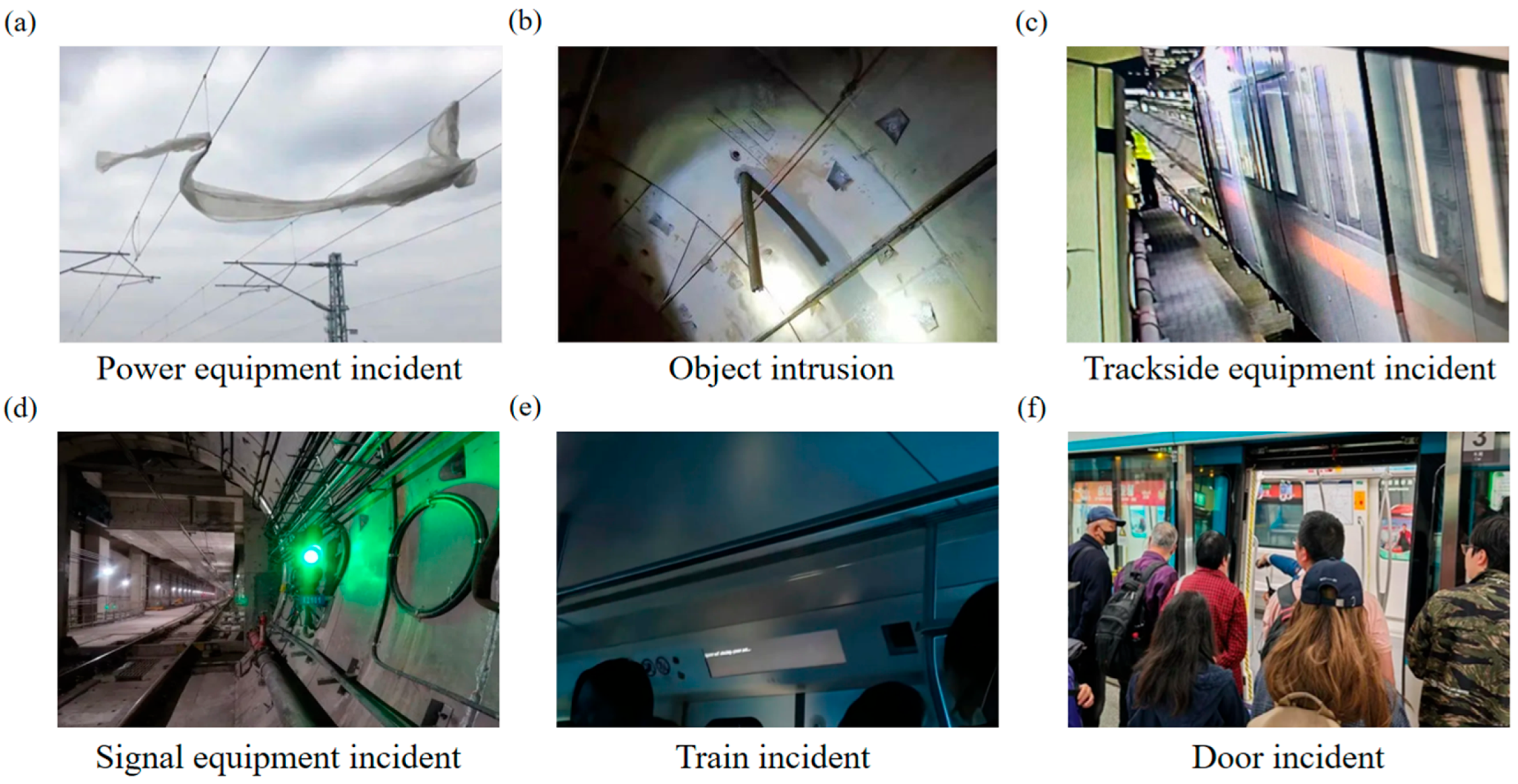Incident-induced disruptions, including equipment incidents, infrastructure damage, natural disasters, and human-related incidents, severely impact urban rail efficiency and reliability [1]. Common subway incidents, such as power equipment failures, trackside equipment faults, signal disruptions, and train malfunctions (see Figure 1), result in varying degrees of service interruption, thereby affecting passenger flow. However, existing research lacks timely and accurate predictions of passenger origin–destination (OD) flows specifically under disrupted conditions, exacerbating congestion and causing cascading impacts across transit networks [2]. Addressing this gap by accurately predicting OD matrices during incidents is critical for enhancing operational resilience and proactive incident management [3,4].

Recently, advanced deep learning (DL) techniques have demonstrated promising results in enhancing passenger OD matrix predictions due to their capability to model complex nonlinear relationships and high-dimensional spatiotemporal data [5,6]. Techniques such as convolutional neural networks (CNNs), recurrent neural networks (RNNs), and even Transformers have shown substantial improvements over traditional models [5,7,8]. However, despite prediction methodological advancements, conventional DL models often struggle with interpretability issues, providing limited insights into the underlying mechanisms driving passenger flow variations during incidents. The lack of interpretability hampers their practical application in operational decision-making scenarios, where understanding the causal relationships and spatiotemporal impacts of disruptions is crucial [9]. Furthermore, due to the scarcity of incident-specific data, it is challenging to simultaneously observe changes in OD matrices under both incident and normal conditions, complicating accurate predictions and causal analysis.

Therefore, to address these research gaps, the objective of this study was to develop an interpretable deep counterfactual inference framework to accurately predict passenger OD matrices under operational disruptions in urban rail systems. Counterfactual inference offers a robust analytical approach for capturing causal relationships and providing interpretable predictions through “what-if” scenario estimation [10,11]. Specifically, we first designed a tensor decomposition model coupled with the Kullback–Leibler (KL) divergence measure to effectively represent and quantify passenger flow dynamics, facilitating robust propensity matching between normal and disrupted conditions. Then, we develop a dual-channel deep counterfactual prediction model based on multi-task learning paradigms, which simultaneously estimates passenger OD matrices under normal operational conditions and counterfactually predicts passenger OD flows under incident-induced disruptions. By quantifying the divergence between the normal-condition and incident-related passenger flows using tensor-based metrics, the proposed framework explicitly models the spatiotemporal dynamics and causal impacts of disruptions, providing interpretable predictions and actionable insights. Empirical analyses conducted using real-world data from Shanghai’s extensive urban rail network demonstrate significant improvements in prediction accuracy under incident conditions compared to baseline models, with Mean Absolute Percentage Error (MAPE) reductions ranging from 40% to 70%, thereby confirming the practical effectiveness of the proposed approach.

Our study contributes to the existing knowledge in three aspects. First, from a theoretical perspective, the proposed dual-channel counterfactual inference model integrates factual predictions with counterfactual estimations, explicitly capturing causal effects and improving predictive robustness during emergency conditions. Second, the interpretability is significantly enhanced by offering quantifiable spatiotemporal differences between factual and counterfactual scenarios. Third, from a practical perspective, this study offers transit operators actionable insights into the real-time impacts of operational disruptions by employing our tools, enabling subway operators to estimate disrupted passenger volumes and swiftly implement emergency operational strategies.

The remainder of this paper is structured as follows. Section 2 reviews related work on urban rail transit passenger flow prediction. Section 3 presents the methodological framework, illustrating the KL divergence metrics and the architecture of our dual-channel deep counterfactual prediction model, respectively. Section 4 presents our case study dataset, empirical results, and comparative analyses. Section 5 discusses implications, operational insights, and potential limitations of our study and concludes the entire study.

2. Literature Review

Research on passenger OD matrix estimation in urban rail transit spans three main methodological paradigms. Classical and data-driven approaches for modeling spatiotemporal flow patterns under normal operations are first reviewed, followed by an examination of recent developments in deep learning and causal inference that enhance both prediction accuracy and interpretability, thereby laying the groundwork for the proposed counterfactual framework.

2.1. Origin–Destination Matrix Estimation and Prediction

Predicting the passenger OD matrices within urban rail transit systems remains challenging primarily due to the spatiotemporally high dimensionality of the problem [12,13]. Existing research approaches can be broadly categorized into three distinct groups: classical models, deep learning (DL) models, and causal inference-based methods.

Classical models primarily rely on dimensionality reduction and assumptions of structural regularity. Huang, et al. [7] and Zheng, et al. [5] have proposed that the OD matrices exhibit low-rank properties, thus reducing the matrices to smaller manageable sizes amenable to traditional autoregressive modeling techniques. Similarly, Xiong, et al. [13] and Zhu, et al. [12] introduced a simplifying assumption that the ratio between station-to-station passenger flows and the total inflow at stations remains relatively constant, thereby significantly simplifying OD estimation once inflow data are known. Additionally, station-level embedding methods have also been applied to overcome dimensionality constraints [14], enhancing prediction effectiveness.

In contrast, deep learning (DL) models have recently garnered substantial attention due to their capability to model high-dimensional and nonlinear spatiotemporal interactions. Temporal modeling typically leverages recurrent architectures, such as Long Short-Term Memory (LSTM) networks, to capture inherent temporal dependencies [15,16]. Other innovative approaches have involved transforms and incorporating periodic characteristics of passenger flows across daily and weekly as different views [17]. Moreover, attention mechanisms have been increasingly integrated into these frameworks to dynamically emphasize significant temporal features [18]. In terms of spatial modeling, convolutional neural networks (CNNs) have been applied to uncover intricate spatial correlations embedded within historical OD matrices [19]. Graph neural networks (GNNs), exemplified by studies [20,21], represent another prevalent approach, effectively modeling relationships among urban rail transit stations. Other research has implemented multi-resolution analysis through wavelet transforms to derive spatial features at varying granularities [22].

Lastly, causal inference-based methods, although less common, offer interpretability through explicit modeling of causal relationships in passenger flows. Such approaches quantify how specific disruptions or external factors influence transit dynamics, enhancing the understanding of system resilience under disruptions. Dual-transformer architectures have also emerged, simultaneously capturing spatial-temporal relationships to improve OD flow predictions [23]. Nevertheless, despite numerous advancements, existing research predominantly emphasizes general operational scenarios, with insufficient exploration of incident and emergency conditions.

2.2. Evaluating Incident Effects on Urban Rail Transit Systems

Silva, et al. [24] developed a predictive model originally for regular operational scenarios that has been adapted as counterfactual tools. These models predict expected passenger flows under normal conditions, providing a baseline against which actual passenger flows during incidents and emergencies are compared, effectively quantifying incidents’ impacts [25]. Additionally, Zou, et al. [9] developed an OD prediction framework explicitly incorporating incidents as variables, enabling comparisons between normal and disrupted conditions and effectively quantifying passenger flow deviations attributable to disruptions. Other targeted models directly predict passenger flow during incidents and emergencies, contrasting them against baseline scenarios to determine impacts [26,27]. Simulation methods further support these analyses, providing estimates of passenger flows at stations experiencing disruptions, thus illuminating detailed incident impacts [28]. Causal inference methods have also been applied to operational data to systematically evaluate subway disruption effects on passenger flows, notably highlighting spillover phenomena [29].

In practical applications, several urban rail systems have implemented real-time OD prediction models to enhance operational resilience during incidents. For instance, the Hong Kong Mass Transit Railway (MTR) has adopted a multi-resolution spatiotemporal deep learning model to forecast OD demand, facilitating dynamic control strategies and passenger information dissemination during unexpected events [30]. These implementations underscore the practical utility of advanced OD prediction models in real-world urban rail operations.

Although significant progress has been made in the prediction of passenger origin–destination (OD) matrices, existing methods ranging from classical models to deep learning (DL) and causal inference-based approaches still face substantial limitations, particularly in the context of operational incidents. Classical methods often simplify the problem by assuming structural regularity or low-rank properties, but these approaches struggle to handle the high-dimensional and dynamic nature of the data. DL models have made strides in capturing nonlinear spatiotemporal dependencies, yet they often lack interpretability, hindering their practical application in emergency scenarios. While causal inference-based methods offer valuable insights into system resilience, they are limited by a focus on general operational conditions, with insufficient exploration of real-time incident impacts. The proposed framework in this study bridges these gaps by integrating deep counterfactual inference, which enhances both prediction accuracy and interpretability. The motivation behind our approach stems from the need to predict OD matrices in real-time during incidents, a scenario largely unexplored by existing methods. By using KL divergence-based propensity matching and a dual-channel architecture, our model captures the spatiotemporal impacts of disruptions and provides interpretable insights into the underlying mechanisms.

3. Methods

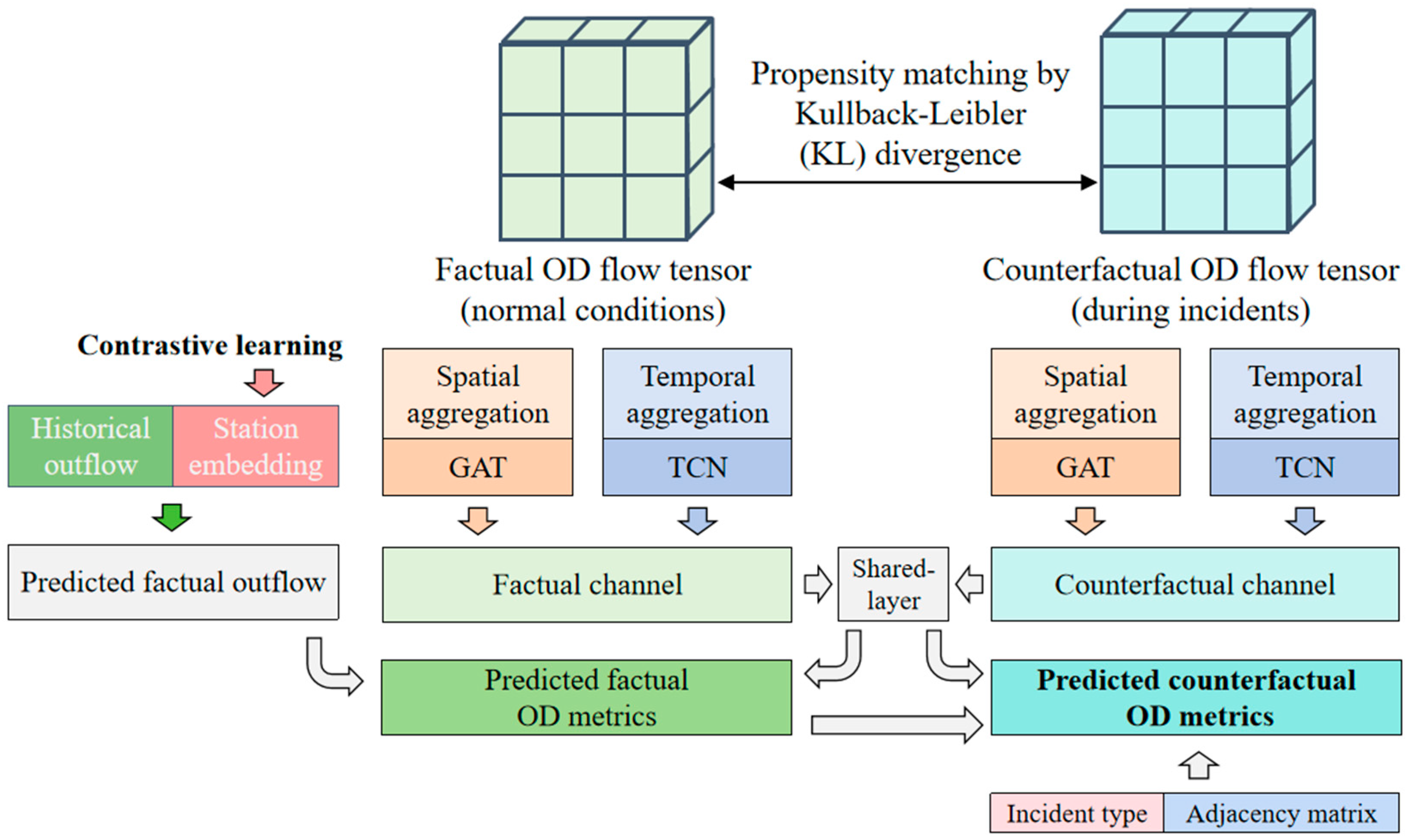
The methodology comprises three integrated stages: propensity matching based on tensor KL-divergence to align each incident scenario with a statistically comparable normal condition and thus isolate causal effects; training a dual-channel deep counterfactual model that fuses shared station embeddings, graph attention, temporal convolutions and incident-type embeddings to capture both baseline and disruption-driven OD flow dynamics; and applying the trained model to generate spatiotemporal passenger-flow predictions under varied incident types while quantitatively assessing how disruptions propagate through the network over time. This framework combines robust predictive accuracy with causal interpretability to support real-time operational decision-making in urban rail systems.

3.1. Research Framework

The proposed framework follows a three-stage process: (1) propensity matching between factual (normal) and counterfactual (incident) scenarios, forming paired input data capturing both normal and disrupted conditions; (2) training of a dual-channel deep counterfactual prediction model; and, (3) once trained, this model allows predictions of spatiotemporal passenger flow dynamics and quantifies causal impacts of operational incidents on passenger distribution across the network. The entire framework is presented as in Figure 2.

To clearly illustrate the method principle of the proposed framework, we define the following terms first.

Definition 1.

Prediction Time Interval: The day is segmented into $T$ intervals of length $\Delta \tau$, typically equals to 10, 20, 30, or 60 min. Let $t\in \{1,2,\dots ,T\}$ index each discrete interval.

Definition 2.

Urban rail transit network graph: The URT network is defined as an undirected graph $G=(V,E)$, where $V$ is the set of URT stations and $E$ is the set of edges representing direct operational connections between stations. An edge $(v_i,v_j)$ exists if there is a direct connection between stations $v_i$ and $v_j$.

Definition 3.

Urban rail transit passenger trip: A passenger trip $\xi$ is characterized by origin station $o$, departure time interval $t_o$, destination station $d$, and arrival interval $t_d$. Individual-level trips are recorded via Automatic Fare Collection (AFC) systems [26].

Definition 4.

Station-level passenger flow: The inflow $I_s^t$ for station $s$ at interval $t$ is the count of passengers entering station $s$ during time interval $t$. Similarly, outflow $O_s^t$ denotes the passengers exiting at station $s$ during time interval $t$. Mathematically, we have:

$$I_s^t={\displaystyle \sum _{\xi }𝕀\left(o=s,t_o=t\right)}$$

(1)

$$O_s^t={\displaystyle \sum _{\xi }𝕀\left(d=s,t_d=t\right)}$$

(2)

Definition 5.

OD flow matrix: The OD passenger flow matrix $F^t\in {\mathit{ℝ}}^{S\times S}$ for interval $t$ captures passengers traveling between each OD pair:

$$F_{ij}^t={\displaystyle \sum _{\xi }𝕀\left(o=v_i,d=v_j,t_o=t\right)}$$

(3)

3.2. Propensity Matching Between Factual and Counterfactual

To accurately quantify the causal effects of operational incidents on passenger origin–destination (OD) flows, it is essential to establish a match between factual scenarios (normal operating conditions) and counterfactual scenarios (conditions under operational disruptions) since we cannot observe the OD passenger flows under factual and counterfactual conditions simultaneously. Specifically, assume a tensor $\mathcal{F}\in {\mathbb{R}}^{S\times S\times T}$ to represent the dynamic evolution of OD passenger flows under factual conditions (normal condition), where $S$ denotes the total number of stations, and $T$ represents the number of discrete prediction intervals within the study period. Each element ${\mathcal{F}}_{ij}^t$ in this tensor reflects the number of passengers traveling from station $i$ to station $j$ during interval $t$ under normal operation.

Similarly, the OD flow dynamics under counterfactual conditions (incident and emergency conditions) are captured by another tensor $\mathcal{C}\in {\mathbb{R}}^{S\times S\times T}$, where each element ${\mathcal{C}}_{ij}^t$ denotes the number of passengers traveling from station $i$ to station $j$ during interval $t$ when an operational incident occurs.

To ensure matched scenarios represent equivalent underlying conditions with minimal confounding differences apart from the operational incident, we adopt propensity matching based on tensor Kullback–Leibler (KL) divergence. KL divergence is an appropriate measure to quantify the dissimilarity between two probability distributions represented by tensors. Formally, the KL divergence between factual tensor $\mathcal{F}$ and counterfactual tensor $\mathcal{C}$ is defined as Equation (4):

$$\mathrm{KL}\left(\mathcal{F}‖\mathcal{C}\right)={\displaystyle \sum _{t=1}^T{\displaystyle \sum _{i=1}^N{\displaystyle \sum _{j=1}^N{\mathcal{F}}_{ij}^t\ln \frac{{\mathcal{F}}_{ij}^t+\epsilon }{{\mathcal{C}}_{ij}^t+\epsilon }}}}$$

(4)

where $\epsilon$ is a small positive constant introduced to avoid division by zero, and $N$ represents the number of stations. A smaller KL divergence indicates a higher similarity between the two tensors, suggesting these scenarios are suitable for pairing.

Paired datasets are constructed by selecting factual scenarios from historical OD flow data that most closely match each counterfactual incident scenario based on the minimum tensor KL divergence criterion. Formally, given an incident scenario tensor ${\mathcal{C}}^{(m)}$, the matched factual tensor ${\mathcal{F}}^{(m)}$ is selected from a candidate set $\{{\mathcal{F}}^{(1)},{\mathcal{F}}^{(2)},\dots ,{\mathcal{F}}^{(N)}\}$ as:

$${\mathcal{F}}^{(m)}=\underset{{\mathcal{F}}^{(n)}}{\arg \min }\mathrm{KL}\left({\mathcal{F}}^{(n)}‖{\mathcal{C}}^{(m)}\right)$$

(5)

Therefore, each incident scenario ${\mathcal{C}}^{(m)}$ is paired with the most similar factual scenario ${\mathcal{F}}^{(m)}$ with the sample index $m$ and $n$. Matched datasets allow deep learning models to distinguish between normal fluctuations and incident-induced deviations in passenger flows. These paired data then serve as input for training the dual-channel deep counterfactual prediction model, effectively capturing and quantifying the causal impact of incidents on passenger OD flows. It should be noted that the matching between factual and counterfactual scenarios does not imply a temporal “before-and-after” implementation; rather, it involves identifying operationally comparable but separate historical conditions. Thus, our methodological design differs from conventional before-and-after comparative analyses.

3.3. Dual-Channel Deep Counterfactual Prediction Model for OD Matrix Prediction

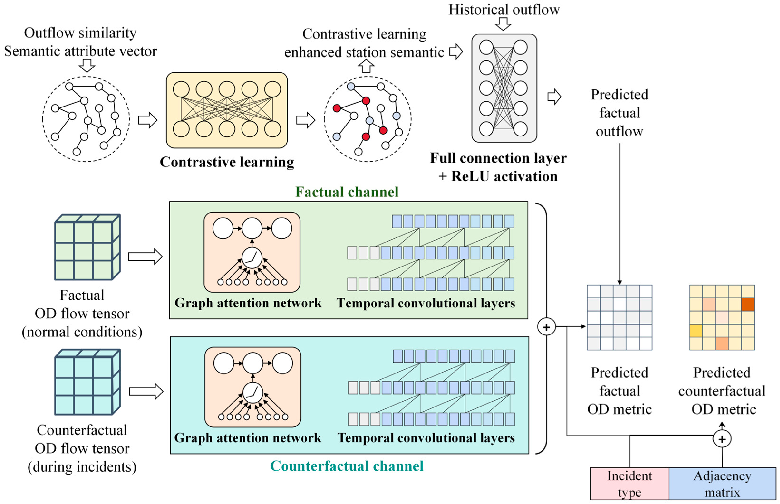
The proposed dual-channel deep counterfactual (DC-DCF) prediction model consists of several core components based on the multi-task learning architectures: (1) the contrastive learning-enhanced URT station semantic extraction as shared layers, (2) the graph attention and temporal convolution for spatiotemporal OD knowledge utilization, (3) the shared layers for factual and counterfactual (incident and emergency conditions) OD matrices prediction, and (4) the incident type embedding module. The network structure is presented as Figure 3.

3.3.1. Shared Contrastive Learning-Enhanced URT Station Semantic Extraction

In the proposed framework, contrastive learning is employed to learn robust URT station embeddings that can capture spatiotemporal interactions between stations. Given that this module serves as a shared layer, its embeddings are used as inputs for both the factual and counterfactual task-specific towers, making it essential for generating consistent, high-quality features for downstream tasks. The semantic attribute vector $S_i$ for each station $i$ is defined by the POI features and location semantics $S=[S_1,S_2,\dots ,S_{l_p}]$, where $l_p$ denotes the largest semantics for URT station. The contrastive learning method is then used to project these semantic attributes into a higher-dimensional embedding space ${\mathcal{S}}_{\mathrm{embedd}}$, where each station is represented by its embedding vector $s_i$. The model then identifies positive and negative station pairs based on the daily outflows sequence, denoted as $O_t=[O_1,O_2,\dots ,O_{l_p}]$, where $O_i$ represents the outflow at station $i$ during time interval $t$. The cosine similarity between the outflow sequences of two stations $i$ and $j$ is defined as Equation (6):

$$\mathrm{Sim}\left(O_i,O_j\right)={\displaystyle \frac{O_i·O_j}{‖O_i‖‖O_j‖}}$$

(6)

Based on the pre-defined similarity thresholds ${\theta }^{+}$ and ${\theta }^{-}$, station pairs are classified into positive or negative pairs. The contrastive loss is defined as Equation (7):

$${\mathcal{L}}_{\mathrm{contractive}}=-{\displaystyle \sum _{i\in S}\ln \frac{e^{s_i·s_{pos}}}{e^{s_i·s_{pos}}+{\displaystyle {\sum }_{j\in S_{neg}}{e}^{s_i·s_j}}}}$$

(7)

where $s_{pos}$ is the embedding of the positive station, $s_j$ are the embeddings of the negative stations, and $S_{\mathrm{neg}}$ is the negative set for each anchor-positive pair. After training, the high-dimensional semantic embeddings $\mathit{E}$ for each station $s_i$ are obtained, which serve as the station-level input features for downstream station-level and OD-level passenger flow prediction tasks.

The semantic embedding vector used in the shared contrastive learning-enhanced URT station semantic extraction process primarily includes static features, such as land use characteristics (e.g., the proportion of different POI types within a 500 m radius around each station) and the presence of transport hubs, central business districts, universities, and public transport stations. Dynamic features such as incident type (dummy variable), peak hours, workday status, and adverse weather conditions, are also considered but are not station-specific and are not part of the shared contrastive learning process.

3.3.2. Factual and Counterfactual OD Passenger Flow Prediction

Define $N$ as the total number of urban rail transit (URT) stations, $T$ as the prediction time window length, $M$ as the station semantic embedding dimension, $H$ as the hidden layer dimension and $K$ as the number of incident types. To explicitly model the spatiotemporal deviations induced by operational incidents, our prediction framework simultaneously integrates factual and counterfactual OD passenger flow tensors, leveraging multiple data sources including shared station semantic embeddings, historical station outflow sequences, incident occurrence indicators, incident type information, and network topology.

Specifically, denote $\mathcal{F}\in {\mathbb{R}}^{N\times N\times T}$ and $\mathcal{C}\in {\mathbb{R}}^{N\times N\times T}$ as factual and counterfactual OD tensors, respectively. Additionally, denote $\mathit{E}\in {\mathbb{R}}^{N\times M}$ as the station semantic embedding obtained via contrastive learning, $\mathit{O}\in {\mathbb{R}}^{N\times T}$ as historical outflow sequences, $\psi \in \{0,1\}$ as the incident indicator (1 for incident scenarios, 0 for normal operations), $\gamma \in {\left\{0,1\right\}}^K$ as the incident-type one-hot encoding vector, and $\mathit{A}\in {\left\{0,1\right\}}^{N\times N}$ as the binary adjacency matrix representing network topology. To capture temporal dynamics and station heterogeneity, the semantic embeddings and historical outflow data for each station are firstly concatenated as follows:

$${\mathit{z}}_i={\mathit{O}}_i\oplus {\mathit{E}}_i\in {\mathbb{R}}^{T+M}$$

(8)

This integrated tensor ${\mathit{z}}_{\mathit{i}}$ is subsequently processed by a two-layer fully connected neural network with ReLU activation to predict station-level passenger outflows at the subsequent time interval:

$${\widehat{\mathit{o}}}_{\mathit{i}}={\mathit{W}}_{\mathit{2}}^{\top }\mathrm{ReLU}\left({\mathit{W}}_{\mathit{1}}{\mathit{z}}_i+{\mathit{b}}_{\mathit{1}}\right)+{\mathit{b}}_{\mathit{2}}$$

(9)

where ${\mathit{W}}_1\in {\mathbb{R}}^{H\times \left(T+M\right)}, {\mathit{W}}_2\in {\mathbb{R}}^H, {\mathit{b}}_1\in {\mathbb{R}}^H$ and ${\mathit{b}}_2\in \mathbb{R}$ denote trainable weight and bias parameters. The resulting outflow predictions inform subsequent OD matrix decomposition by providing station-level passenger volume constraints. For capturing OD-specific spatiotemporal correlations, spatial and temporal features are derived from historical OD tensors as follows:

$${\mathit{U}}^F={\displaystyle {\sum }_{t=1}^T{\mathcal{F}}_{i,j,t}},\forall i,j\in I\wedge i\ne j$$

(10)

$${\mathit{U}}^{CF}={\displaystyle {\sum }_{t=1}^T{\mathcal{C}}_{i,j,t}},\forall i,j\in I\wedge i\ne j$$

(11)

$${\mathit{V}}^F={\displaystyle {\sum }_{j=1}^N{\mathcal{F}}_{i,j,t}},\forall i\in I\wedge t\in T\wedge i\ne j$$

(12)

$${\mathit{V}}^{CF}={\displaystyle {\sum }_{j=1}^N{\mathcal{C}}_{i,j,t}},\forall i\in I\wedge t\in T\wedge i\ne j$$

(13)

Here, ${\mathit{U}}^F$ and ${\mathit{U}}^{CF}$ represent spatial aggregation, while ${\mathit{V}}^F$ and ${\mathit{V}}^{CF}$ represent temporal aggregation under factual and counterfactual conditions, respectively. To dynamically model shifts in spatial dependencies due to operational disruptions, a graph-attention layer re-weights station adjacency relation:

$${\mathit{\alpha }}_{\mathit{i},\mathit{j}}^F={\displaystyle \frac{exp\left({\left({\mathit{W}}_{GAT}{\mathit{U}}_i^F\right)}^{\top }\left({\mathit{W}}_{GAT}{\mathit{U}}_j^F\right)\right)}{{\displaystyle {\sum }_{k=1}^{N}exp\left({\left({\mathit{W}}_{GAT}{\mathit{U}}_i^F\right)}^{\top }\left({\mathit{W}}_{GAT}{\mathit{U}}_k^F\right)\right)}}},{\mathit{U}}^F={\displaystyle {\sum }_{j=1}^N{\mathit{\alpha }}_{\mathit{i},\mathit{j}}^F\left({\mathit{W}}_{GAT}^{\prime }{\mathit{U}}_j^F\right)}$$

(14)

$${\mathit{\alpha }}_{\mathit{i},\mathit{j}}^{CF}={\displaystyle \frac{exp\left({\left({\mathit{W}}_{GAT}{\mathit{U}}_i^{CF}\right)}^{\top }\left({\mathit{W}}_{GAT}{\mathit{U}}_j^{CF}\right)\right)}{{\displaystyle {\sum }_{k=1}^{N}exp\left({\left({\mathit{W}}_{GAT}{\mathit{U}}_i^{CF}\right)}^{\top }\left({\mathit{W}}_{GAT}{\mathit{U}}_k^{CF}\right)\right)}}},{\mathit{U}}^{CF}={\displaystyle {\sum }_{j=1}^N{\mathit{\alpha }}_{\mathit{i},\mathit{j}}^{CF}\left({\mathit{W}}_{GAT}^{\prime }{\mathit{U}}_j^{CF}\right)}$$

(15)

where ${\mathit{W}}_{GAT}$ and ${\mathit{W}}_{GAT}^{\prime }$ denote trainable parameters. Simultaneously, temporal convolutional layers capture periodic patterns:

$${\mathit{V}}^F=ReLU\left(Convld({\mathit{V}}^F)\right)\in {\mathbb{R}}^{N\times T}$$

(16)

$${\mathit{V}}^{CF}=ReLU\left(Convld({\mathit{V}}^{CF})\right)\in {\mathbb{R}}^{N\times T}$$

(17)

The extracted spatiotemporal embeddings from both factual and counterfactual channels are concatenated:

$$\mathit{H}=\left({\mathit{U}}^F\oplus {\mathit{U}}^{CF}\right)\oplus \left({\mathit{V}}^F\oplus {\mathit{V}}^{CF}\right)\in {\mathbb{R}}^{2N+2T}$$

(18)

These embeddings are projected linearly to obtain OD flow estimations:

$${\mathit{H}}^{\prime }={\mathit{W}}_{proj}\mathit{H}+{\mathit{b}}_{proj}\in {\mathbb{R}}^{N\times N}$$

(19)

$${\widehat{\mathit{X}}}^F=\mathrm{ReLU}\left({\mathit{W}}^F\left({\mathit{H}}^{\prime }\odot \widehat{\mathit{o}}\right)+{\mathit{b}}_f\right)$$

(20)

For the counterfactual scenario, the embedding vector $\mathit{\delta }={\widehat{\mathit{X}}}^F\oplus {\mathit{A}}_{ij}\oplus \left(\psi \oplus \gamma \right)\in {\mathbb{R}}^{K+3}$ is similarly processed through a dedicated two-layer neural network to yield OD predictions conditioned explicitly on incident characteristics:

$${\widehat{\mathit{X}}}^{CF}=\mathrm{ReLU}\left({\mathit{W}}_2^{CF}\mathrm{ReLU}\left({\mathit{W}}_1^{CF}\mathit{\delta }+{\mathit{b}}_1^{CF}\right)+{\mathit{b}}_2^{CF}\right)$$

(21)

This modeling approach explicitly incorporates incident conditions, facilitating precise “what-if” scenario reasoning for proactive incident management.

3.3.3. Loss Function and Prediction Accuracy Evaluation Metrics

The dual-channel deep counterfactual prediction model is trained using a two-stage training strategy to effectively handle data sparsity and the distribution shifts between factual (normal) and counterfactual (incident-induced) scenarios. Both stages utilize Mean Squared Error (MSE) loss functions with added regularization terms to prevent overfitting and enhance model generalization.

In the initial training stage, only factual data are employed to optimize the shared embedding parameters and the factual prediction branch parameters. The loss function is formulated as follows:

$${\mathcal{L}}_1={\displaystyle \frac{1}{\left|{\mathcal{D}}^F\right|}}{\displaystyle \sum _{\left({\widehat{\mathit{X}}}^F,{\mathit{X}}^F\right)\in {\mathcal{D}}^F}{‖{\widehat{\mathit{X}}}^F-{\mathit{X}}^F‖}_2^2}+\lambda {‖\mathrm{\Theta }‖}_2^2$$

(22)

where ${\stackrel{⌢}{\mathit{X}}}^F$ represents the predicted OD passenger flow under factual conditions, ${\mathit{X}}^F$ is the ground-truth OD flow matrix in normal operating scenarios, ${\mathcal{D}}^F$ denotes the set of factual training samples, $\mathrm{\Theta }$ denotes the trainable model parameters for regulation term, and $\lambda$ is the regularization coefficient.

In the subsequent training stage, counterfactual data are incorporated to jointly optimize both factual and counterfactual branches. The loss function is expanded to simultaneously minimize prediction errors under both conditions, defined as:

$${\mathcal{L}}_2={\displaystyle \frac{1}{\left|{\mathcal{D}}^F\right|}}{\displaystyle \sum _{\left({\widehat{\mathit{X}}}^F,{\mathit{X}}^F\right)\in {\mathcal{D}}^F}{‖{\widehat{\mathit{X}}}^{CF}-{\mathit{X}}^{CF}‖}_2^2}+{\displaystyle \frac{1}{\left|{\mathcal{D}}^{CF}\right|}}{\displaystyle \sum _{\left({\widehat{\mathit{X}}}^F,{\mathit{X}}^F\right)\in {\mathcal{D}}^{CF}}{‖{\widehat{\mathit{X}}}^{CF}-{\mathit{X}}^{CF}‖}_2^2}+\lambda \left({‖{\mathrm{\Theta }}^F‖}_2^2+{‖{\mathrm{\Theta }}^{CF}‖}_2^2\right)$$

(23)

where ${\stackrel{⌢}{\mathit{X}}}^{CF}$ is the counterfactual prediction, ${\mathit{X}}^{CF}$ represents the observed OD flows under incident scenarios, ${\mathcal{D}}^{CF}$ is the set of counterfactual samples, and $\mathrm{\Theta }$ denote trainable parameters specific to factual and counterfactual prediction branches.

To evaluate the model’s predictive accuracy specifically under counterfactual (incident) scenarios, three metrics are adopted: Mean Absolute Error (MAE), Mean Absolute Percentage Error (MAPE), and Root Mean Square Error (RMSE). The corresponding formulas are defined as follows:

$$\mathbf{M}\mathbf{A}\mathbf{E}={\displaystyle \frac{1}{\left|{\mathcal{D}}^{CF}\right|}}{\displaystyle \sum _{\left({\widehat{\mathit{X}}}^F,{\mathit{X}}^F\right)\in {\mathcal{D}}^{CF}}\left|{\widehat{\mathit{X}}}^{CF}-{\mathit{X}}^{CF}\right|}$$

(24)

$$\mathbf{M}\mathbf{A}\mathbf{P}\mathbf{E}={\displaystyle \frac{1}{\left|{\mathcal{D}}^{CF}\right|}}{\displaystyle \sum _{\left({\widehat{\mathit{X}}}^F,{\mathit{X}}^F\right)\in {\mathcal{D}}^{CF}}\left|\frac{{\widehat{\mathit{X}}}^{CF}-{\mathit{X}}^{CF}}{{\mathit{X}}^{CF}}\right|}\times 100\%$$

(25)

$$\mathbf{R}\mathbf{M}\mathbf{S}\mathbf{E}=\sqrt{ }{\displaystyle \frac{1}{\left|{\mathcal{D}}^{CF}\right|}}{\displaystyle \sum _{\left({\widehat{\mathit{X}}}^F,{\mathit{X}}^F\right)\in {\mathcal{D}}^{CF}}{\left({\widehat{\mathit{X}}}^{CF}-{\mathit{X}}^{CF}\right)}^2}$$

(26)

These metrics provide comprehensive assessments of prediction errors in magnitude, proportional accuracy, and sensitivity to large deviations. The pseudocode for model training algorithm is provided in Algorithm 1.

Algorithm 1: Dual-channel deep counterfactual prediction model
Input:
	Factual data $\mathcal{F}\in {\mathbb{R}}^{N\times N\times T}$ (OD flows under normal conditions)
	Counterfactual data $\mathcal{C}\in {\mathbb{R}}^{N\times N\times T}$ (OD flows during incidents)
	Model architecture $\mathrm{\Theta }$ with dual channels (factual and counterfactual)
	Regularization coefficient $\lambda$ for model optimization
Output:
	Trained DC-DCF model weights
Stage 1: Factual condition training
01.	Initialize model parameters: weights $\mathit{W}$, biases $\mathit{b}$, embeddings $\mathit{E}$
02.	Prepare factual OD flow tensor (passenger flows under normal conditions)
03.	Define factual loss function ${\mathcal{L}}_1$(MSE) with regularization
04.	For each training iteration do:
05.	Input factual data: station semantics, historical outflows, OD tensors
06.	Concatenate input features
07.	Pass through factual channel:
08.	(a) Predict station-level outflows via fully connected layers
09.	(b) Aggregate spatial features via GAT
20.	(c) Extract temporal patterns via TCN
21.	(d) Concatenate spatiotemporal embeddings
22.	(e) Predict OD matrix
23.	Calculate factual loss: MSE(factual prediction, ground truth)
24.	Backpropagate error and update model parameters
25.	Repeat until convergence
Stage 2: Factual-counterfactual joint training
21.	Prepare factual and counterfactual OD flow tensor
22.	Define loss function ${\mathcal{L}}_2$ for both channel (MSE)
23.	For each training iteration do:
24.	Input factual data: station embeddings, OD tensor, outflows
25.	Input counterfactual data: OD tensor, incident indicators, incident types
26.	Process both channels:
27.	(a) Factual prediction (repeat steps 10–17)
28.	(b) Counterfactual prediction
29.	i. Combine inputs
30.	ii. Pass through counterfactual network layers
31.	iii. Predict OD matrix:
32.	- Spatial aggregation
33.	- Temporal modeling
34.	- Concatenation
35.	- Output via two-layer MLP
36.	Calculate factual loss: MSE(factual prediction, factual ground truth)
37.	Calculate counterfactual loss: MSE(counterfactual prediction, counterfactual ground truth)
38.	Calculate total loss: total_loss = factual_loss + counterfactual_loss
39.	Backpropagate error and update model parameters
40.	Repeat until convergence
41.	Evaluate performance using MAE, MAPE, and RMSE on counterfactual validation/test set
Return The trained DC-DCF model weights and evaluation metrics

4. Results

The analysis describes the study area and dataset and then presents a systematic evaluation of model performance. Prediction accuracy is assessed across multiple temporal granularities and passenger-flow conditions using MAE MAPE and RMSE. Ablation experiments quantify the impact of key methodological components including KL divergence-based propensity matching graph contrastive embeddings and incident-type features. A detailed analysis of incident categories uncovers heterogeneous delay characteristics and spatiotemporal propagation phenomena that underscore the model’s operational relevance.

4.1. Study Area and Dataset

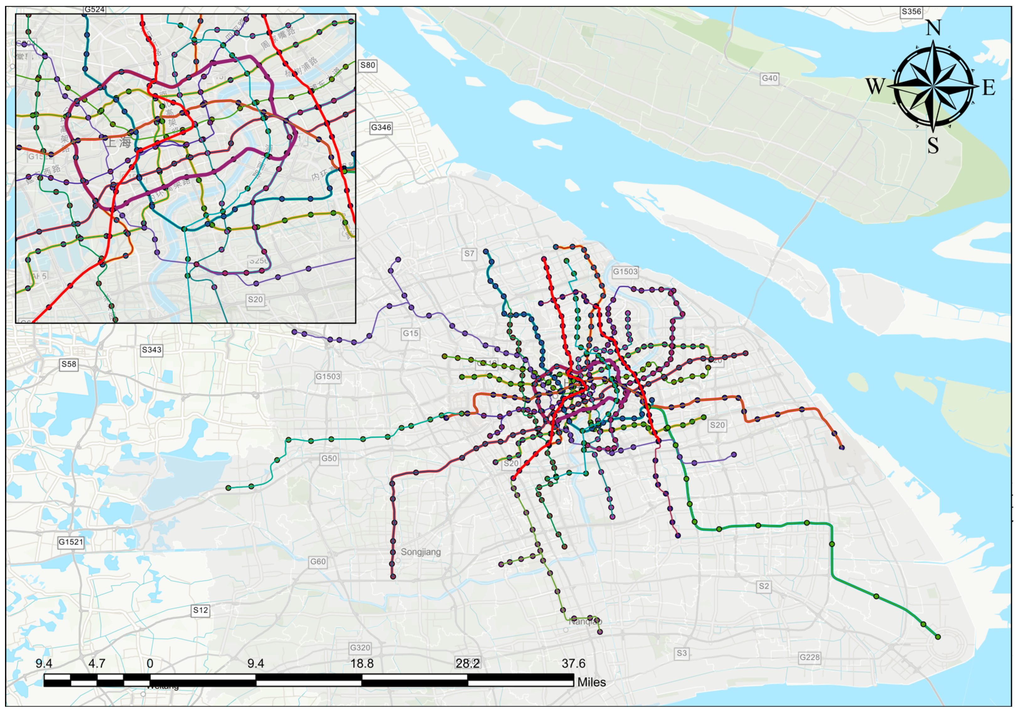
This research focuses on the Shanghai URT system, comprising 20 lines and 409 stations. With an average daily ridership of approximately 11.41 million passengers on weekdays, the system faces significant challenges in optimizing operational resources and improving service quality. This study integrates multiple datasets to model passenger flow patterns and the effects of operational disruptions, including the Shanghai URT smartcard dataset, land use data, and multimodal public transport network data. The lines and stations distribution of Shanghai urban rail transit network are presented as Figure 4.

The Shanghai URT smartcard dataset covers weekdays and weekends from 6:00 AM to 10:00 PM, spanning the period from 1 September to 28 September 2023. For the temporal analysis, the dataset is divided into four time intervals per day: 96 intervals for 10 min segments, 48 intervals for 20 min segments, 32 intervals for 30 min segments, and 16 intervals for 60 min segments. The dataset is split into training, validation, and testing sets with a ratio of 70%, 20%, and 10%, respectively, for both factual and counterfactual samples. This study divides sub-networks from the complex Shanghai URT system. These sub-networks are selected based on different passenger flow conditions: high passenger flow, medium passenger flow, and low passenger flow. The specific composition, mileage, and station number for each sub-network are outlined in

Table 1. Network composition, mileage, and station number of the study cases.

Study Case	Network Composition	Network Mileage	Number of Stations
High passenger flow	Line-1, Line-2, Line-9	163.14 km	90
Medium passenger flow	Line-3, Line-12, Line-13	119.59 km	88
Low passenger flow	Line-6, Line-7, Line-16	136.42 km	72

.

Figure 5 illustrates the weekly variation in passenger flow under normal conditions for each sub-network. The flow patterns exhibit clear cyclical behavior, with significant peaks during weekdays and more irregular, lower-level distributions on weekends. The high passenger flow group consistently shows notably higher ridership levels on weekends compared to the medium and low passenger flow groups.

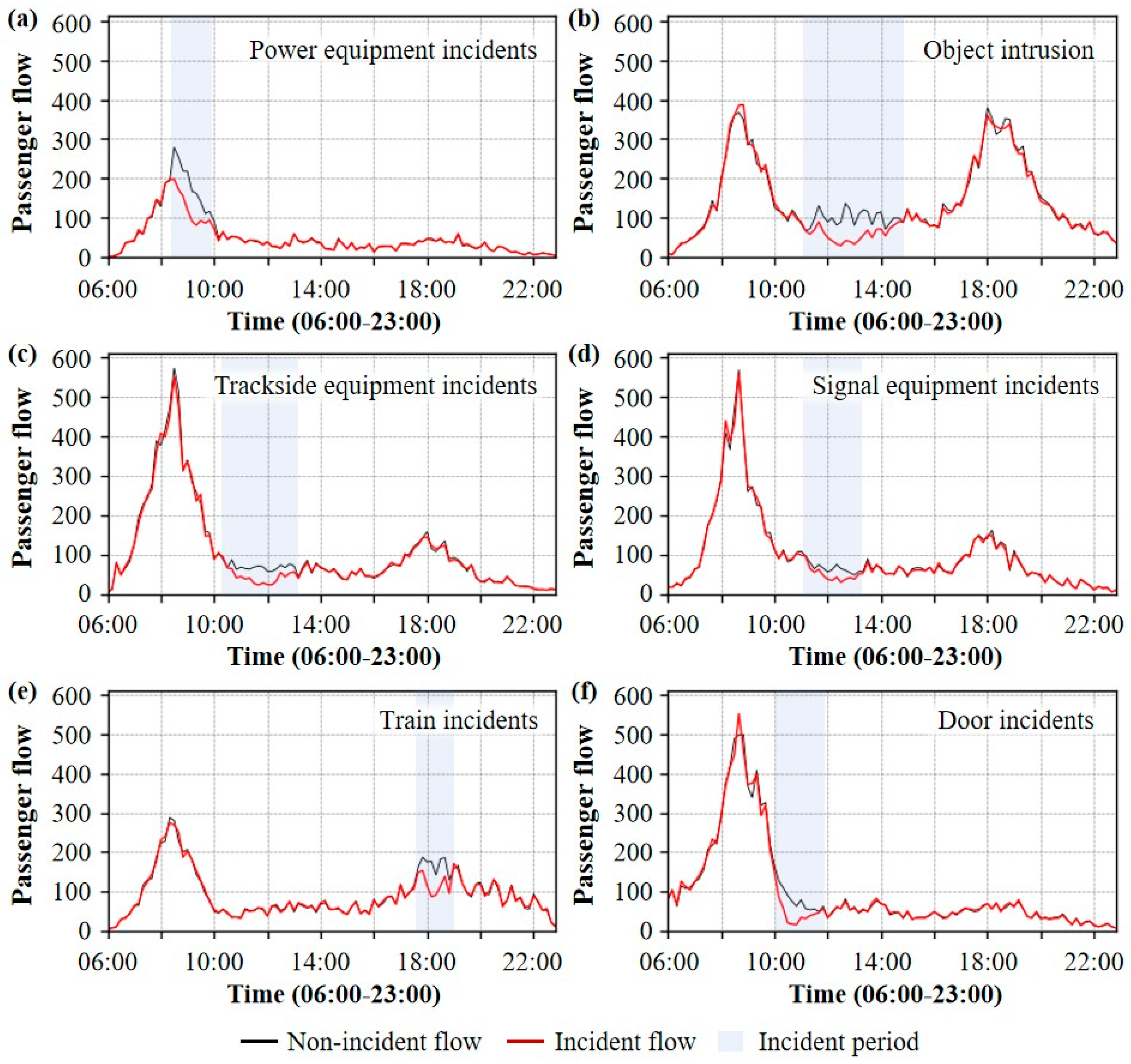
Specifically, incidents included in the datasets are categorized as follows: Power equipment incidents (5.4%), Object intrusion (3.8%), Trackside equipment incidents (6.6%), Signal equipment incidents (25.8%), Train incidents (30.2%), and Door incidents (28.2%). The incident datasets were randomly divided into training, validation, and testing subsets with proportions of 70%, 20%, and 10%, respectively. A descriptive analysis of passenger flow patterns under various incident conditions was included to clearly demonstrate the real-world relevance and potential applicability of our model, as in Figure 6.

In terms of land use semantics, this study incorporates Points of Interest (POI) data within a 500 m radius around each OD pair’s origin and destination stations. These POIs are categorized into work, residential, education, healthcare, and commercial entertainment. Additionally, proximity to key land use features, such as universities, central business districts (CBDs), transport hubs, and bus stations, is considered. The corresponding data, shown in Figure 7, reveals significant differences in land use patterns across the three passenger flow groups. The high flow group tends to be located closer to densely populated areas such as CBDs and transport hubs, whereas the medium and low flow groups exhibit more varied land use characteristics. Commercial and entertainment POIs are the most common across all sub-networks, though the high flow group demonstrates a stronger concentration of these POIs near transport hubs and central business districts.

It should be noted that this study employs a two-stage training approach. The first stage uses a dataset of OD flows from a continuous week of normal operations, representing factual conditions (non-incident). The second stage incorporates data on URT incidents and passenger flow disruptions collected over the past five years. This integration of incident data enables the prediction of passenger flows during operational disruptions.

4.2. Hyperparameter Configuration and Computational Setup

The hyperparameter configuration of the proposed dual-channel deep counterfactual model is presented as

Table 2. Hyperparameter configuration of the dual-channel deep counterfactual model.

Parameter Name	Description	Value
Embedding Dimension	Dimension of station semantic embeddings	64
Hidden Layer Dimension	Dimension of hidden layers in neural networks	128
Number of GAT Heads	Number of attention heads in the Graph Attention Network (GAT)	8
GAT Output Dimension per Head	Output dimension of each GAT head	16
TCN Kernel Size	Kernel size of the temporal convolution layers	3
Number of TCN Layers	Number of layers in the temporal convolution network	2
First MLP Layer Dimension	Dimension of the first layer in the final MLP decoder	128
Second MLP Layer Dimension	Dimension of the second layer in the final MLP decoder	64
Dropout Rate	Dropout rate applied to avoid overfitting	0.3
Activation Function	Activation function used in all hidden layers	ReLU
Learning Rate	Initial learning rate for the optimizer	0.001
Optimizer Type	Optimization algorithm used for training	Adam
Batch Size	Number of samples per batch	64
Number of Training Epochs	Number of training epochs	100
Weight Decay Coefficient	Weight decay (L2 regularization coefficient)	0.0001
Early Stopping Patience	Number of epochs to wait before early stopping	10
Gradient Clipping Threshold	Gradient clipping threshold to prevent explosion	5
Shuffle Training Data	Whether to shuffle training data each epoch	True
Validation Split Ratio	Proportion of training data used for validation	0.1
Random Seed	Random seed for reproducibility	42

. The model’s architectural design includes a station embedding dimension of 64, which is sufficient to capture semantic and locational attributes without incurring excessive parameterization. The hidden layers within the network are set to a dimension of 128, ensuring adequate capacity to model complex nonlinear relationships among features. The graph attention mechanism utilizes eight attention heads, each producing an output dimension of 16, which collectively enhances the model’s ability to capture diverse spatial dependencies across the transit network. Temporal dependencies are extracted through a two-layer temporal convolutional network with a kernel size of three, enabling the model to learn sequential patterns across adjacent time intervals effectively.

To support the transformation of high-dimensional spatiotemporal representations into OD flow predictions, a two-layer multilayer perceptron is employed in the decoder. The first and second layers of the MLP are set to 128 and 64 dimensions respectively, enabling a gradual reduction in feature space complexity prior to output. A dropout rate of 0.3 is applied across hidden layers as a regularization strategy to mitigate overfitting, especially given the potential sparsity in counterfactual observations. The rectified linear unit is used as the activation function throughout the architecture, given its widespread success in deep learning applications due to non-saturating gradients and computational efficiency.

Training procedures were conducted using the Adam optimizer with a learning rate of 0.001, a setting commonly adopted for stable and efficient convergence in temporal graph-based networks. A mini-batch size of 64 was selected to balance computational tractability with variance reduction in gradient estimates. The model was trained for up to 100 epochs, with early stopping applied if validation loss fails to improve over 10 consecutive epochs, thereby reducing the risk of overfitting. To further regularize the model, weight decay was implemented with a coefficient of 0.0001, penalizing large weights and encouraging smoother solutions. Gradient clipping with a threshold of 5.0 was used to prevent exploding gradients during backpropagation, ensuring numerical stability during optimization. Training data were shuffled at the start of each epoch, and a validation split of 10 percent was reserved to monitor generalization performance. A fixed random seed of 42 was used to ensure the reproducibility of experimental results across runs and environments.

4.3. Prediction Results

Experiments were conducted to evaluate prediction accuracy across different time scales and passenger flow conditions using MAE, MAPE, and RMSE metrics. Computational time and accuracy with marginal changes in network size are presented in Appendix A 

Table A1. Computational time and accuracy with marginal changes in network size.

Network Scale	Computational Time (h)	10 min MAPE	20 min MAPE	30 min MAPE	60 min MAPE
3 lines	12.165	6.437	8.905	10.587	13.849
4 lines	22.601	6.587	9.937	11.305	14.590
5 lines	34.576	7.591	10.036	12.399	15.601
6 lines	49.140	8.205	10.846	13.581	18.064
7 lines	63.953	9.076	12.660	14.532	19.739

. The core observation is that prediction errors in the high passenger flow scenario are consistently larger than those in the medium and low flow scenarios. This is primarily due to the higher fluctuation and wider variation in passenger flows under high flow conditions, which makes accurate predictions more challenging. Larger time scales tend to result in higher prediction errors compared to smaller time scales. However, the increase in MAE and RMSE is proportional to the time scale, suggesting that the error mainly reflects the impact of time granularity on the model’s performance. In contrast, the MAPE metric does not increase proportionally. The reason for this discrepancy is that as the base value for comparison grows with the time scale, the relative prediction error becomes less significant.

For instance, as illustrated in

Table 3. Prediction accuracy of counterfactual OD passenger flow in different cases and time scales.

Time Scale	High Passenger Flow Case			Medium Passenger Flow Case			Low Passenger Flow Case
	MAE	MAPE	RMSE	MAE	MAPE	RMSE	MAE	MAPE	RMSE
10 min	0.773 **	6.437 **	4.518 **	0.210 **	2.105 ***	1.887 **	0.176 ***	1.850 ***	1.504 ***
20 min	1.559 **	8.905 *	8.981 **	0.421 **	3.167 **	3.522 **	0.358 ***	2.801 **	2.811 **
30 min	2.347 *	10.587 *	13.368 **	0.648 *	4.013 **	5.347 **	0.526 **	3.995 **	3.437 **
60 min	4.655 *	13.849 *	25.642 *	1.268 *	5.654 **	9.821 *	1.036 **	4.907 **	7.201 **

To evaluate the concentration and statistical significance of the prediction results, we assess the proportion of predicted samples that fall within three times the standard deviation (±3σ) of the prediction errors for each evaluation metric, namely Mean Absolute Error (MAE), Mean Absolute Percentage Error (MAPE), and Root Mean Square Error (RMSE). Based on the coverage ratio within this interval, significance levels are categorized as follows: a coverage of 99% or higher is marked with ***, 95% to 99% with **, and 90% to 95% with *.

, the MAE for the high passenger flow case increases from 0.773 at the 10 min scale to 4.655 at the 60 min scale. At the same time, the MAPE increases from 6.437% at the 10 min scale to 13.849% at the 60 min scale, which demonstrates that the relative error increases less dramatically. Similarly, the RMSE increases from 4.518 at the 10 min scale to 25.642 at the 60 min scale, confirming the trend that larger time scales tend to amplify prediction errors, particularly in high flow scenarios. Statistical significance tests were also conducted to assess the concentration of prediction errors for MAE, MAPE, and RMSE by calculating the percentage of samples within ±3σ of each error distribution. Across all passenger flow cases and time scales, the coverage ratios consistently exceed 90%, indicating robust performance. The low passenger flow case exhibits the highest significance levels, followed by the medium and high flow cases, suggesting that reduced flow variability yields more concentrated predictions. Shorter time intervals (10 min and 20 min) demonstrate higher coverage proportions than longer intervals (30 min and 60 min), reflecting the greater absolute variation inherent in larger time scales.

A comparison of the proposed dual-channel deep counterfactual (DC-DCF) model with several baseline models was also performed under the 10 min time scale. These baseline models included LSTM+GCN, LSTM+GAT, and TCN, along with a Transformer model that encodes incident features but lacks the dual-channel counterfactual component. In addition, Deep Twin Networks for counterfactuals estimation [11] which incorporates counterfactual structure but uses a different data matching approach, was included for comparison. The results, presented in

Table 4. Comparison of prediction accuracy across different algorithms under 10 min scale.

Algorithms	High Passenger Flow Case			Medium Passenger Flow Case			Low Passenger Flow Case
	MAE	MAPE	RMSE	MAE	MAPE	RMSE	MAE	MAPE	RMSE
LSTM+GCN	2.193	19.419	13.361	0.655 *	7.142 *	5.483	0.551 *	5.335 **	4.645 *
LSTM+GAT	2.218	20.824	13.273	0.692 *	5.987 *	5.569 *	0.510 **	6.198 **	4.462 *
TCN	2.370 *	19.514 **	12.051 *	0.557 *	6.592 *	5.519 *	0.529 **	5.260 *	4.466 **
Transformer	1.600 *	13.682 *	11.334 *	0.490 **	4.914 **	4.183 **	0.400 **	3.831 **	3.626 *
Deep Twins	1.367 ***	11.197 ***	8.467 ***	0.372 ***	3.729 ***	3.531 ***	0.343 ***	3.589 ***	2.566 ***
DC-DCF	0.773 **	6.437 **	4.518 **	0.210 **	2.105 ***	1.887 **	0.176 ***	1.850 ***	1.504 ***

Note: LSTM stands for Long Short-Term Memory network, GCN stands for Graph Convolutional Network, GAT stands for Graph Attention Network, TCN stands for temporal convolutional network, Transformer is based on attention mechanisms for OD passenger flow prediction, and Deep Twins represents Deep Twin Networks for Categorical Counterfactuals Estimation. DC-DCF stands for the dual-channel deep counterfactual OD passenger flow prediction model proposed in this study. Coverage of 99% or higher is marked with ***, 95% to 99% with **, and 90% to 95% with *.

, reveal that the baseline models like LSTM+GCN and LSTM+GAT exhibit higher errors across all passenger flow conditions compared to DC-DCF, particularly in high passenger flow scenarios. LSTM-based models (LSTM+GCN, LSTM+GAT) show the poorest performance. This is attributable to their reliance on consistent temporal patterns, which are disrupted during incidents, causing significant prediction bias. Although the Transformer model improves over the baseline models due to its encoding of incident features, it still underperforms compared to DC-DCF. The Deep Twins and DC-DCF models, both of which integrate factual and counterfactual data, perform significantly better. Among these, the DC-DCF model, which leverages KL divergence-based propensity matching, outperforms Deep Twins, demonstrating the effectiveness of the fact-counterfactual data matching mechanism developed in this study.

The ablation experiments further support the importance of the components within the DC-DCF framework. The results shown in

Table 5. Ablation experiment of dual-channel deep counterfactual OD passenger flow prediction model under 10 min scale.

Ablation Combination	High Passenger Flow Case			Medium Passenger Flow Case			Low Passenger Flow Case
	MAE	MAPE	RMSE	MAE	MAPE	RMSE	MAE	MAPE	RMSE
Condition 1	2.155 ***	17.922 ***	11.393 ***	0.494 ***	5.481 ***	4.535 ***	0.491 ***	5.133 ***	3.756 ***
Condition 2	1.501 ***	11.577 ***	7.936 ***	0.364 ***	3.560 ***	3.453 ***	0.303 ***	3.377 ***	2.792 ***
Condition 3	1.186 ***	11.002 ***	7.812 ***	0.366 ***	3.410 ***	3.285 ***	0.301 ***	2.907 ***	2.208 ***
Condition 4	1.383 ***	10.064 ***	7.242 ***	0.367 ***	3.847 ***	2.986 ***	0.285 ***	2.938 ***	2.544 ***
Condition 5	2.116 ***	16.596 ***	12.305 ***	0.512 ***	4.857 ***	4.932 ***	0.455 ***	4.746 ***	3.709 ***
Condition 6	2.391 ***	20.133 ***	13.118 ***	0.661 ***	5.932 ***	6.057 ***	0.546 ***	5.426 ***	4.383 ***
DC-DCF	0.773 **	6.437 **	4.518 **	0.210 **	2.105 ***	1.887 **	0.176 ***	1.850 ***	1.504 ***

Note: condition 1 is the experiment with no matching and paired datasets; condition 2 is the experiment with no contrastive learning-enhanced URT station semantic extraction; condition 3 is the experiment with no graph-attention layer for spatial knowledge utilization; condition 4 is the experiment with no convolutional layer for temporal knowledge utilization; condition 5 is the experiment with no shared layer for factual and counterfactual knowledge learning; condition 6 is the experiment with no incident type knowledge embedded. Coverage of 99% or higher is marked with ***, 95% to 99% with **.

validate the necessity of several key components, such as the fact–counterfactual passenger flow tensor matching, graph-based contrastive learning for station semantics, the GAT layer for spatial knowledge updating, the temporal convolutional layers for time-based learning, the shared layer for collaborative learning of factual and counterfactual information, and the incident type embedding feature. The experiments emphasize that the inclusion of incident type knowledge embedding, fact-counterfactual tensor matching, and the shared layer are the most critical elements for optimal model performance. The removal of fact–counterfactual propensity matching produces the largest performance drop. Without matched factual reference samples, the counterfactual channel lacks a reliable baseline for estimating passenger flow deviations and results in greater prediction errors. To assess the statistical significance of the differences between Condition 2 and Condition 3, we calculated the sample coverage within the ±3 standard deviation range. The results showed that Condition 2 (no contrastive learning-enhanced URT station semantic extraction) yielded a higher coverage of 94.265%, 96.291%, and 98.373% for the high, medium, and low passenger flow cases, respectively, compared to Condition 3 (no graph-attention layer for spatial knowledge utilization), which had a coverage of 90.117%, 93.772%, and 95.165% across the same cases. These results indicate that the removal of contrastive learning has a more differentiated impact on prediction accuracy compared to the removal of the graph-attention layer.

4.4. Incident’s Impact on OD Flows Analysis

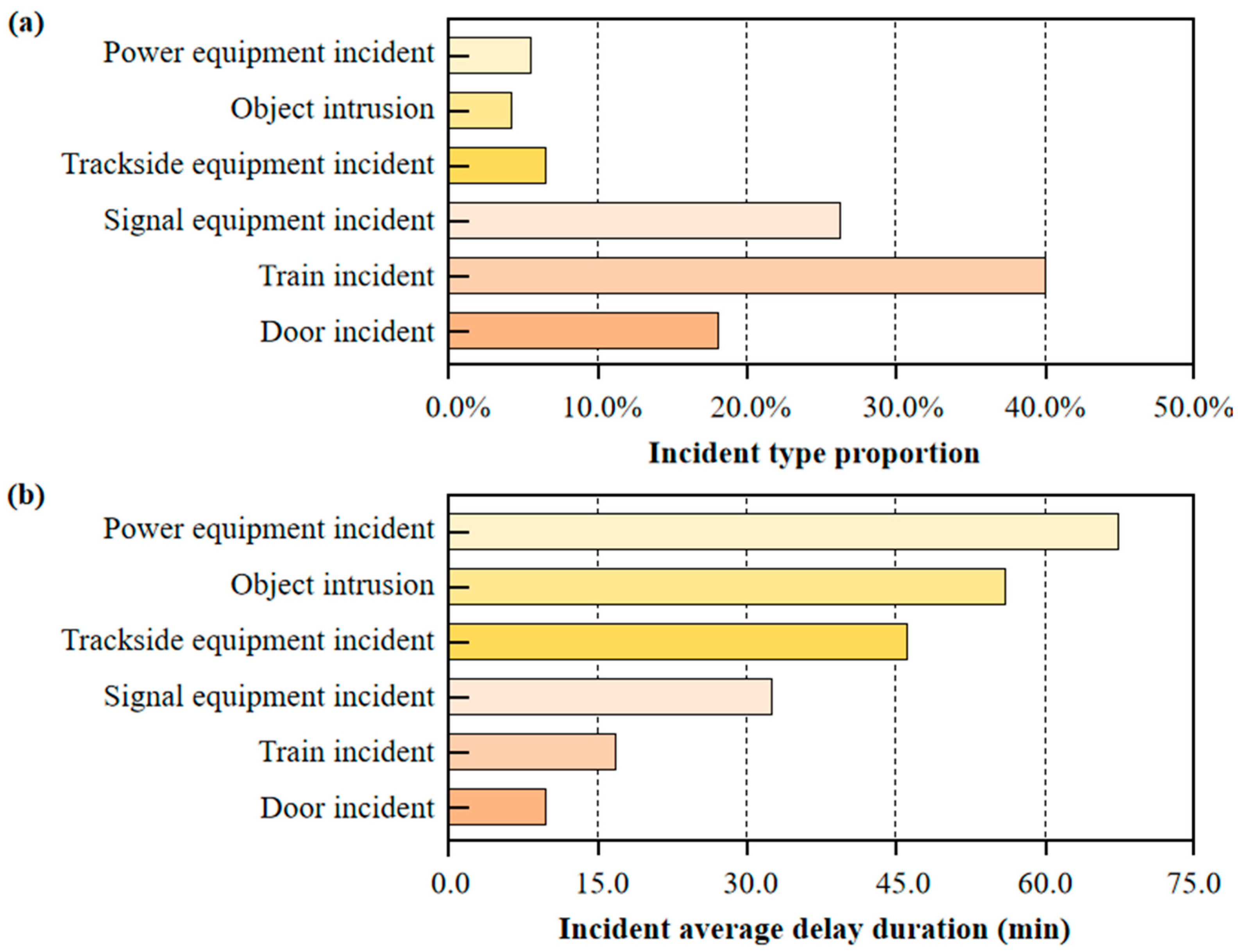
The effectiveness of the DC-DCF model is further confirmed through a detailed analysis of the impact of various incident types on short-term OD passenger flow trends. Six primary incident types are considered in this study: power equipment incidents, object intrusion, trackside equipment incidents, signal equipment incidents, train incidents, and door incidents. The proportion of each incident type and its associated average delay duration are computed and displayed in Figure 8. The analysis reveals an inverse relationship between the incident frequency and the average delay duration caused by each type. Train incidents, the most common incident type, accounts for nearly 40% of all incidents but results in an average delay of only 16 min. In contrast, power equipment incidents, which occurs in fewer than 5% of cases, causes an average delay of approximately 70 min. These findings highlight the significant heterogeneity between incident occurrence probabilities and the consequences of each incident type.

The trained DC-DCF model is applied to predict the average impact of each incident type on OD flows, both for OD pairs involving the incident station as the origin and destination and for those involving neighboring stations. The results, presented in

Table 6. Short-term passenger flow impacts of different incident types on OD passenger flow of incident stations.

Incident Type	Post-Incident Period	Incident-Station Origin OD Pairs	Incident-Station Destination OD Pairs
Power equipment incidents	30 min	−67.392%	−42.685%
	60 min	−75.579%	−59.530%
Object intrusion	30 min	−62.040%	−34.822%
	60 min	−60.483%	−51.499%
Trackside equipment incidents	30 min	−48.330%	−29.020%
	60 min	−48.804%	−39.874%
Signal equipment incidents	30 min	−32.218%	−19.929%
	60 min	−34.935%	−29.420%
Train incidents	30 min	−17.654%	−9.399%
	60 min	−17.154%	−13.676%
Door incidents	30 min	−10.340%	−6.016%
	60 min	−11.638%	−8.461%

and

Table 7. Short-term passenger flow impacts of different incident types on the OD passenger flow of neighboring stations.

Incident Type	Post-Incident Period	OD Pairs of Adjacent Stations as the Origin	OD Pairs of Adjacent Stations as the Destination
Power equipment incidents	30 min	−22.934%	−12.888%
	60 min	−26.623%	−18.349%
Object intrusion	30 min	−17.539%	−11.355%
	60 min	−19.622%	−15.373%
Trackside equipment incidents	30 min	−12.836%	−9.096%
	60 min	−16.433%	−10.580%
Signal equipment incidents	30 min	−10.308%	−4.853%
	60 min	−11.004%	−8.022%
Train incidents	30 min	−5.128%	−2.721%
	60 min	−4.750%	−5.682%
Door incidents	30 min	−2.889%	−1.695%
	60 min	−3.363%	−2.462%

The percentages presented in Table 6 and Table 7 were calculated based on the following distribution of incident types: Power equipment incidents (5.4%), Object intrusion (3.8%), Trackside equipment incidents (6.6%), Signal equipment incidents (25.8%), Train incidents (30.2%), and Door incidents (28.2%).

, confirm the heterogeneous nature of the impact of different incidents on OD flows, as well as the spatial propagation of these effects. The findings show that incidents significantly reduce passenger flow for OD pairs associated with the affected station and its neighboring stations. For OD pairs where the affected station serves as the origin, the impact is almost instantaneous, as the disruption directly affects the current time period. Conversely, when the affected station serves as the destination, the impact is delayed due to the time required for the negative effects of delays to propagate across the network.

The influence of incidents on neighboring stations is also significant but lower in magnitude compared to the affected station, and this effect is subject to a time-lag. The study further establishes a clear positive correlation between the duration of the negative impact on passenger flow and the time required for the incident to be resolved. For example, power equipment incidents, which takes the longest to resolve, results in the most substantial decrease in OD passenger flows, with a reduction of −93.729%. On the other hand, door incidents, which is easier to repair, leads to a smaller decrease in OD passenger flows, with a loss of only −14.120%. These results emphasize the critical role of the time required to address each incident in determining the extent of its impact on the overall network performance. The longer the resolution time, the more severe the disruption to passenger flow, highlighting the need for efficient and timely incident management.

5. Discussion

Given these findings, several policy implications emerge. It is crucial for subway systems to develop a tiered emergency response system for different incident types. Incidents such as power equipment incidents and object intrusion, which cause significant delays, should be classified as first-level incidents, while trackside equipment incidents and signal equipment incidents should be second-level, and train incidents and door incidents should be third-level incidents. These tiers would enable the implementation of tailored emergency measures, such as directing passengers to waiting areas for repair, implementing flow diversion to prevent overcrowding, or initiating bus connections. Additionally, modeling the spatiotemporal changes in passenger flow at neighboring stations can help identify stations likely to be impacted by the incident, allowing for early warnings and preemptive safety measures to prevent the escalation of the disruption’s effects.

Transit agencies worldwide are beginning to explore AI-driven decision support tools, and a model like this could be integrated into their operations control centers for live scenario evaluation. For instance, one recent framework combining deep learning and incident information demonstrated substantially improved detection of ridership drops during disruptions [9]. By deploying similar predictive systems, a metro operator could automatically anticipate the magnitude of passenger displacement caused by an incident and initiate timely interventions. Another advantage of our counterfactual approach is its transparency: because the model separately estimates what would have happened in the absence of the incident, staff can directly compare the predicted “normal” versus “incident-affected” OD matrices. Such comparisons make the impact of the disruption immediately interpretable to planners and controllers, and they can see which origin–destination flows are most affected and by how much, rather than just receiving a single opaque forecast. This interpretability builds trust in the model’s suggestions and aligns with the goal of improving situational awareness during crises [21].

The predictive capabilities of our model can be instrumental in real-time operational decision-making. For example, if the model forecasts a significant increase in passenger flow at a particular station due to an incident, transit operators can proactively add train runs or deploy shuttle buses to alleviate congestion. Similarly, if a station is predicted to become a bottleneck, temporary closure or controlled access measures can be implemented to ensure passenger safety and maintain service reliability.

In practical terms, the enhanced interpretability and modular design (each channel serving a distinct role) mean the tool could function as a reliable “advisor” to human decision-makers, who remain accountable for service adjustments. Real-world use cases could include scenario analysis (e.g., “If a certain station must close for 30 min, what are the expected OD flow changes and where should we allocate extra buses?”) and post-incident analysis (“How much did this disruption divert trips or suppress demand compared to normal?”). By providing data-driven answers to these questions, the model can assist transit agencies in not only reacting to incidents but also learning from them to improve resilience.

6. Conclusions

6.1. Conclusions

This research introduces a novel approach to predicting passenger origin–destination (OD) matrices during operational disruptions in urban rail systems. A dual-channel deep counterfactual inference model is developed, integrating factual predictions with counterfactual estimations to predict passenger flows under both normal and incident conditions. This model explicitly enhances predictive robustness in the face of emergencies. The design of key components, such as tensor-based KL divergence for propensity matching between factual and counterfactual conditions, a shared layer for synergistic learning of knowledge across both channels, and the integration of incident type embedding features are critical innovations that improve model performance and interpretability. Our study makes three primary contributions. From a theoretical perspective, the dual-channel counterfactual inference model offers a sophisticated way to account for the causal effects of disruptions. From an interpretability standpoint, it provides valuable insights into spatiotemporal differences between normal and disrupted scenarios. Practically, it equips transit operators with actionable tools to assess real-time disruption impacts and implement effective emergency responses.

Among the most significant insights of this study is the demonstration that KL divergence–based propensity matching can reliably utilize normal and disrupted passenger flow patterns, yielding a nuanced understanding of temporal disruption trends. Equally important is the incorporation of incident-type embeddings, which captures the heterogeneous delay effects most notably, the disproportionately large impact of power equipment failures compared to more frequent but less severe incidents. The analysis reveals consistent time-lag propagation, where disruptions immediately depress origin station flows, while destination and neighboring stations experience delayed and attenuated effects. These findings not only advance the theoretical framework for OD prediction under incident conditions but also offer actionable guidance for real-time operational adjustments in urban rail networks.

6.2. Limitation and Future Works

However, this research still has several limitations. While our model demonstrates promising results using Shanghai’s urban rail transit data, we recognize the necessity of validating its applicability across different urban settings. Future research will focus on applying and testing the model in other cities, such as Beijing, Shenzhen, and London, to assess its generalizability and adaptability to various transit systems and operational conditions. Additionally, the model does not consider detailed incident characteristics, such as specific fault locations or causes, and does not account for the network-level propagation of delays. Future research could integrate detailed fault modeling and network-level delay propagation to improve the accuracy of the predictions.

Although the deep counterfactual inference framework proposed in this study performs well in simulation environments, we have not yet been able to deploy and test the model in real operations of the Shanghai Metro due to the complexity of the actual operational environment and limitations in data acquisition. Therefore, direct comparison data before and after the model implementation is not available. Future research should aim to work with metro operators to conduct field tests to verify the model’s effectiveness in real operations and further optimize the model for real-world applications. We fully acknowledge that our study is currently based on historical data and simulations, without examples of real-time deployment during specific disruptions. This limitation, common in academic research contexts, indeed restricts direct assessments of operational impacts, such as enabling earlier decisions for incident management strategies.

References

- Sun, H.; Wu, J.; Wu, L.; Yan, X.; Gao, Z. Estimating the influence of common disruptions on urban rail transit networks. Transp. Res. Part A Policy Pract. 2016, 94, 62–75. [Google Scholar] [CrossRef]
- Lu, Q.-C. Modeling network resilience of rail transit under operational incidents. Transp. Res. Part A Policy Pract. 2018, 117, 227–237. [Google Scholar] [CrossRef]
- Zuo, T.; Tang, S.; Zhang, L.; Kang, H.; Song, H.; Li, P. An Enhanced TimesNet-SARIMA Model for Predicting Outbound Subway Passenger Flow with Decomposition Techniques. Appl. Sci. 2025, 15, 2874. [Google Scholar] [CrossRef]
- Hou, Z.; Han, J.; Yang, G. Analysis of Passenger Flow Characteristics and Origin–Destination Passenger Flow Prediction in Urban Rail Transit Based on Deep Learning. Appl. Sci. 2025, 15, 2853. [Google Scholar] [CrossRef]
- Zheng, F.; Zhao, J.; Ye, J.; Gao, X.; Ye, K.; Xu, C. Metro OD matrix prediction based on multi-view passenger flow evolution trend modeling. IEEE Trans. Big Data 2022, 9, 991–1003. [Google Scholar] [CrossRef]
- Li, D.; Cao, J.; Li, R.; Wu, L. A spatio-temporal structured LSTM model for short-term prediction of origin-destination matrix in rail transit with multisource data. IEEE Access 2020, 8, 84000–84019. [Google Scholar] [CrossRef]
- Huang, D.; Yu, J.; Shen, S.; Li, Z.; Zhao, L.; Gong, C. A method for bus OD matrix estimation using multisource data. J. Adv. Transp. 2020, 2020, 5740521. [Google Scholar] [CrossRef]
- Cao, Y.; Li, X. Multi-Model Attention Fusion Multilayer Perceptron Prediction Method for Subway OD Passenger Flow under COVID-19. Sustainability 2022, 14, 14420. [Google Scholar] [CrossRef]
- Zou, L.; Wang, Z.; Guo, R. Real-time prediction of transit origin–destination flows during underground incidents. Transp. Res. Part C Emerg. Technol. 2024, 163, 104622. [Google Scholar] [CrossRef]
- Prosperi, M.; Guo, Y.; Sperrin, M.; Koopman, J.S.; Min, J.S.; He, X.; Rich, S.; Wang, M.; Buchan, I.E.; Bian, J. Causal inference and counterfactual prediction in machine learning for actionable healthcare. Nat. Mach. Intell. 2020, 2, 369–375. [Google Scholar] [CrossRef]
- Vlontzos, A.; Kainz, B.; Gilligan-Lee, C.M. Estimating categorical counterfactuals via deep twin networks. Nat. Mach. Intell. 2023, 5, 159–168. [Google Scholar] [CrossRef]
- Zhu, G.; Ding, J.; Wei, Y.; Yi, Y.; Xu, S.S.D.; Wu, E.Q. Two-Stage OD flow prediction for emergency in urban rail transit. IEEE Trans. Intell. Transp. Syst. 2024, 25, 920–928. [Google Scholar] [CrossRef]
- Xiong, J.; Sun, Y.; Sun, J.; Wan, Y.; Yu, G. Sparse Temporal Data-Driven SSA-CNN-LSTM-Based Fault Prediction of Electromechanical Equipment in Rail Transit Stations. Appl. Sci. 2024, 14, 8156. [Google Scholar] [CrossRef]
- Han, L.; Ma, X.; Sun, L.; Du, B.; Fu, Y.; Lv, W.; Xiong, H. Continuous-Time and Multi-Level Graph Representation Learning for Origin-Destination Demand Prediction. In Proceedings of the 28th ACM SIGKDD Conference on Knowledge Discovery and Data Mining, Washington, DC, USA, 14–18 August 2022; pp. 516–524. [Google Scholar]
- Chu, K.-F.; Lam, A.Y.; Li, V.O. Deep multi-scale convolutional LSTM network for travel demand and origin-destination predictions. IEEE Trans. Intell. Transp. Syst. 2019, 21, 3219–3232. [Google Scholar] [CrossRef]
- Gui, Z.; Sun, Y.; Yang, L.; Peng, D.; Li, F.; Wu, H.; Guo, C.; Guo, W.; Gong, J. LSI-LSTM: An attention-aware LSTM for real-time driving destination prediction by considering location semantics and location importance of trajectory points. Neurocomputing 2021, 440, 72–88. [Google Scholar] [CrossRef]
- Huang, B.; Ruan, K.; Yu, W.; Xiao, J.; Xie, R.; Huang, J. ODformer: Spatial–temporal transformers for long sequence Origin–Destination matrix forecasting against cross application scenario. Expert Syst. Appl. 2023, 222, 119835. [Google Scholar] [CrossRef]
- Geng, M.; Li, J.; Xia, Y.; Chen, X.M. A physics-informed transformer model for vehicle trajectory prediction on highways. Transp. Res. Part C Emerg. Technol. 2023, 154, 104272. [Google Scholar] [CrossRef]
- Zhang, H.; He, J.; Bao, J.; Hong, Q.; Shi, X. A hybrid spatiotemporal deep learning model for short-term metro passenger flow prediction. J. Adv. Transp. 2020, 2020, 4656435. [Google Scholar] [CrossRef]
- Wang, S.; Lv, Y.; Peng, Y.; Piao, X.; Zhang, Y. Metro traffic flow prediction via knowledge graph and spatiotemporal graph neural network. J. Adv. Transp. 2022, 2022, 2348375. [Google Scholar] [CrossRef]
- Wang, X.; Zhang, Y.; Zhang, J. Large-Scale Origin–Destination Prediction for Urban Rail Transit Network Based on Graph Convolutional Neural Network. Sustainability 2024, 16, 10190. [Google Scholar] [CrossRef]
- Wang, K.; Zhan, J.; Si, Q.; Li, Y.; Kong, Y. Dynamic multi-scale spatio-temporal graph ODE for metro ridership prediction. In Proceedings of the 2024 IEEE 7th Advanced Information Technology, Electronic and Automation Control Conference (IAEAC), Chongqing, China, 15–17 March 2024; Volume 7, pp. 1501–1509. [Google Scholar]
- Liu, L.; Zhu, Y.; Li, G.; Wu, Z.; Bai, L.; Lin, L. Online metro origin-destination prediction via heterogeneous information aggregation. IEEE Trans. Pattern Anal. Mach. Intell. 2022, 45, 3574–3589. [Google Scholar] [CrossRef] [PubMed]
- Silva, R.; Kang, S.M.; Airoldi, E.M. Predicting traffic volumes and estimating the effects of shocks in massive transportation systems. Proc. Natl. Acad. Sci. USA 2015, 112, 5643–5648. [Google Scholar] [CrossRef]
- Liu, L.; Chen, J.; Wu, H.; Zhen, J.; Li, G.; Lin, L. Physical-virtual collaboration modeling for intra-and inter-station metro ridership prediction. IEEE Trans. Intell. Transp. Syst. 2020, 23, 3377–3391. [Google Scholar] [CrossRef]
- Xu, X.; Zhang, K.; Mi, Z.; Wang, X. Short-term passenger flow prediction during station closures in subway systems. Expert Syst. Appl. 2024, 236, 121362. [Google Scholar] [CrossRef]
- Ni, M.; He, Q.; Gao, J. Forecasting the subway passenger flow under event occurrences with social media. IEEE Trans. Intell. Transp. Syst. 2016, 18, 1623–1632. [Google Scholar] [CrossRef]
- Su, G.; Si, B.; Zhi, K.; Zhao, B.; Zheng, X. Simulation-based method for the calculation of passenger flow distribution in an urban rail transit network under interruption. Urban Rail Transit 2023, 9, 110–126. [Google Scholar] [CrossRef]
- Zeng, J.; Zhang, G.; Rong, C.; Ding, J.; Yuan, J.; Li, Y. Causal learning empowered OD prediction for urban planning. In Proceedings of the 31st ACM International Conference on Information & Knowledge Management, Atlanta, GA, USA, 17–21 October 2022; pp. 2455–2464. [Google Scholar]
- Noursalehi, P.; Koutsopoulos, H.N.; Zhao, J. Dynamic origin-destination prediction in urban rail systems: A multi-resolution spatio-temporal deep learning approach. IEEE Trans. Intell. Transp. Syst. 2021, 23, 5106–5115. [Google Scholar] [CrossRef]
Figure 1.
Common types of urban rail transit system incidents.
Figure 2.
Framework for URT network OD matrix prediction under operational incidents. (GAT stands for Graph Attention Network; TCN stands for temporal convolutional network).
Figure 3.
Network structure of the dual-channel deep counterfactual prediction model.
Figure 4.
Line and station distribution of the Shanghai urban rail transit network.
Figure 5.
Weekly passenger flow variation trend in different cases under factual scenarios. This Figure illustrates the weekly variation in passenger flow under normal conditions for each sub-network: (a) High passenger flow case, (b) Mid passenger flow case, and (c) Low passenger flow case. The flow patterns exhibit clear cyclical behavior, with significant peaks during weekdays and more irregular, lower-level distributions on weekends. The high passenger flow group consistently shows notably higher ridership levels on weekends compared to the medium and low passenger flow groups.
Figure 6.
Daily passenger flow variation trend in different cases under incident scenarios. This figure shows the passenger flow patterns under different incident conditions. (a) represents Power equipment incidents, accounting for 5.4% of the total incidents; (b) represents Object intrusion, accounting for 3.8%; (c) represents Trackside equipment incidents, accounting for 6.6%; (d) represents Signal equipment incidents, accounting for 25.8%; (e) represents Train incidents, accounting for 30.2%; (f) represents Door incidents, accounting for 28.2%. The incident datasets were randomly divided into training, validation, and testing subsets with proportions of 70%, 20%, and 10%, respectively. The black line is Non-incident flow, the red line is Incident flow, and the blue area is Incident period, demonstrating the real-world relevance and potential applicability of the model through descriptive analysis of passenger flow patterns under various incident conditions.
Figure 7.
Descriptive statistics of land use types around stations in different cases.
Figure 8.
Incident type proportion and average delay duration.
Figure 8 displays the proportion of each incident type and its associated average delay duration. (
a) Shows the proportion of six incident types (power equipment incidents, object intrusion, trackside equipment incidents, signal equipment incidents, train incidents, door incidents) in all incidents. (
b) Presents the average delay duration (in minutes) corresponding to each of these six incident types. The analysis reveals an inverse relationship between the incident frequency and the average delay duration caused by each type. Train incidents, the most common incident type, accounts for nearly 40% of all incidents but results in an average delay of only 16 min. In contrast, power equipment incidents, which occurs in fewer than 5% of cases, causes an average delay of approximately 70 min.