Optimizing an LSTM Self-Attention Architecture for Portuguese Sentiment Analysis Using a Genetic Algorithm

Featured Application

Automatic sentiment analysis for restaurant reviews.

Abstract

A sentiment analysis is a Natural Language Processing (NLP) task that identifies the opinion or emotional tone of documents such as customer reviews, either at the general or detailed level. Improving domain-specific models is important, as it provides smaller and better-suited models that can be implemented by entities that own textual data. This paper presents a deep learning model trained on Portuguese restaurant reviews using recurrent and self-attention mechanisms, which have consistently delivered strong results in prior research studies. Designing an effective model involves numerous hyperparameters and architectural choices. To address this complexity, a discrete genetic algorithm was used to find an optimal configuration, selecting the layer types, placement of self-attention, dropout rate, and model dimensions and shape. A key outcome of this study was that the optimization process produced a model that is competitive with a Bidirectional Encoder Representation from Transformers (BERT) model retrained for Portuguese, which was used as the baseline. The proposed model achieved an area under the curve of 92.1% and F1-score of 75.4%, demonstrating that a small, optimized model can compete and even outperform larger state-of-the-art models. Moreover, this work helps address the scarcity of NLP resources for Portuguese, and highlights the potential of customized architectures over generic solutions.

1. Introduction

The Internet generates a massive amount of data daily, much of which is textual information ranging from formal, partially structured content found in news articles and informative blogs to the informal, subjective, ironic, and sarcastic text common on social media platforms. Analyzing this type of data is challenging even for humans, as it heavily depends on context. Businesses receive substantial information from social media and their applications, such as customer feedback and reviews, although managing this overwhelming volume can be difficult and may compromise the quality of the service provided. In the restaurant industry, for instance, popular reservation and online ordering platforms such as Zomato allow customers to leave reviews and ratings, enabling restaurant owners to extract valuable insights to assess whether their products and services meet customer expectations.

A sentiment is a feeling, emotion, or opinion expressed through thoughts, words, or actions. Sentiment analysis (SA) is a subfield of natural language processing (NLP) in active development that focuses on automating the extraction and classification of opinions and primarily centers on the valence of emotions, categorizing them as positive, negative, or neutral. It deals with the challenge of understanding the literal meaning of words, their contextual and semantic roles, and the author’s intentions to classify the sentiments expressed.

Deep learning (DL) models constitute the current state of the art for solving complex natural language tasks by extracting patterns from processed text [1,2,3]. Today, large language models (LLMs) trained on vast non-domain-specific datasets allow enterprises to perform natural language tasks with some ease. However, the resulting models are usually large and considerably resource-demanding, becoming difficult to run locally and highly costly to train on graphics processing units (GPUs) [4]. Hence, it is relevant to develop models prepared for specific tasks to optimize their performance and reduce hardware requirements, providing advantages in terms of data safety, enhanced interpretability, and ownership of the model.

This study investigates the document-level SA using Portuguese data and proposes a model based on recurrent mechanisms and self-attention mechanisms to represent text data and extract contextual information. Despite Portuguese being among the top five most spoken languages in the world, with approximately 171 million Internet users (representing 3.7% of all users) [5], limited research has been conducted on this language. Nevertheless, in recent years, there has been an increased number of publications addressing NLP problems in the Portuguese language, primarily focusing on Brazilian Portuguese, and to a lesser extent European Portuguese. The lack of linguistic resources is the main reason for this, leading to most studies focusing on providing resources.

The most relevant surveys in the literature regarding broad NLP applications were published by Ferrone and Zanzotto [6] in 2020, Otter et al. [7] in 2021, Khurana et al. [3] in 2022, and Mao et al. [8] in 2024. They compared various DL models and provided a walk-through of their evolution, overviewing their architectures and describing current state-of-the-art trends and challenges. Furthermore, Pereira [9] performed an extensive survey of multiple approaches to sentiment analysis tasks in Portuguese, including rule-based, conventional machine learning, and deep learning. A main gap that was identified is that most approaches started with English and then adapted to Portuguese, instead of having a model that was developed and optimized in Portuguese from the start. Such was the main goal of this work, where we intended to develop a model in Portuguese text, optimized by a genetic algorithm (GA).

Otter et al. [7] provided a brief overview of the most relevant techniques in NLP tasks, highlighting that SA models are becoming increasingly popular in using DL techniques, with the current state-of-the-art model being an ensemble model that includes convolutional neural networks (CNNs) and long short-term memory (LSTM). Khurana et al. [3], in conformity with Otter et al. [7], stated that artificial neural networks (ANNs) are preferred by researchers in most NLP tasks, with the primary task being text representation in a vectorized dense form. LSTM- and BiLSTM-based models are the latest approaches preferred over CNNs. Additionally, the development of pre-trained models such as BERT, a transformer language model (TLM), allowed fine-tuning for tasks such as SA or question answering (QA) using transfer learning (TL) techniques [3,10]. Finally, Mao et al. [8] discussed in their most recent survey the most relevant datasets and metrics used for the evaluation of SA models. They found that researchers prefer to use domain-specific lexicons to solve SA problems, and conventional machine learning (ML) and DL only when they need to overcome limitations from the previous model.

The most relevant architectures found in recent studies are constituted by LSTM, BiLSTM, CNN, or transformer layers, which benefit from high accuracy by mapping long-term dependencies and focusing on the most relevant terms of the input sequence [11,12]. Some researchers have made efforts to train this model using large datasets from other languages, emphasizing the Portuguese variations of interest in this study, such as BERTimbau [13] and Albertina PT-* [14]. The lack of studies in languages other than English was also highlighted by Khurana et al. [3] and is proposed for future work.

The central studies that introduce and characterize the landscape and developments on SA models for the Portuguese language were driven by Pereira [9] and Souza et al. [15]. The former performed a systematic mapping review up to 2014 and discovered that almost all available language resources were from Brazilian and European Portuguese variations. The encountered studies mainly investigated sentiment classification at the document level and used logistic regression (LR), naïve Bayes (NB), and support vector machine (SVM) models with at least one type of text pre-processing task. The latter made a survey of SA studies in Portuguese, mainly from Portugal and Brazil, which stated the need for new proposals of models for the Portuguese language to better tackle the language specificities. The survey analyzed the whole spectrum of solutions, including lexicon-based approaches, classical ML approaches, and DL approaches, which incorporate CNNs, LSTMs, and transformers.

Souza and Souza Filho [16] reunited five known Brazilian datasets and analyzed them in terms of size, number of n-grams, and length of reviews. They concluded that these Portuguese datasets are less rich in vocabulary than English datasets. Therefore, complex algorithms for Portuguese datasets may not provide the same performance gain when compared to English datasets. Additionally, Brum and Nunes [17] introduced the Brazilian dataset TweetSentBR, which was manually labeled as positive, negative, and neutral by seven native speakers of Brazilian Portuguese. Gomes et al. [18] introduced the dataset BRTweetSentCorpus, manually labeled as positive, negative, ambiguous, and non-opinionated. This process is considerably time-consuming and is not reasonable for larger datasets. Several studies are based on consumer reviews along with a numerical value indicating a rating evaluation between 1 and 5 stars. Dos Santos and Ladeira [19] presented an empirical foundation for this heuristic, applying a t-Student test to verify the comparability of the star rating with a manual classification performed by a human. The result indicated that the star rating is equivalent to manual classification, allowing reliable usage for training an ML algorithm.

Text representation is a fundamental step that enables automatic feature selection and feature engineering. In this context, researchers have mainly used two approaches: bag-of-words (BoW) and contextualized word embedding. Souza and Souza Filho [16,20] compared Word2Vec, GloVe, and FastText vectors trained from the Núcleo Interinstitucional de Linguística Computacional (NILC) word embedding repository [21] on a downstream SA task and found that the embedding technique and its dimensionality have a profound impact on the model performance. Additionally, they analyzed how reliable the representation of FastText-300 was along with LSTM, CNN, and TLM architectures for embedding generation, suggesting that fine-tuned BERTimbau weights provide the best classification performance, slightly better than LSTM and CNN, as also verified by Vianna et al. [22] when compared with GloVe, Word2Vec, and FastText. Regardless, the authors prefer BoW techniques due to their implementation simplicity [17,19,23,24].

Cardoso et al. [23] presented an ensemble approach combining decision trees, NB, SVM, and LR for binary classification, attaining an accuracy rate of 82%. Souza et al. adopted a binary LR classification model with word vector embeddings to attain an ROC-AUC of 94.8% [16] and an LR model to assess the classification performance when using embedding generated by fine-tuned BERTimbau, attaining a score of 97.3% [20]. Both results were obtained from training with multiple-domain datasets. Adán-Coello and Neto [25] optimized a CNN binary classification model using a grid search algorithm and attained an average performance of 82% in accuracy.

Britto et al. [26] performed a similar analysis, exploring other classical ML approaches such as LR, NB, RF, and SVM and comparing them to BERTimbau, also considering the three-class classification scenario (polarity with a neutral class). Their conclusions suggest that the BERT model outperforms in every data domain, although the imbalance of the classes produces a detriment on minority classes, which can be easily seen by the 74% F1-score. Brum and Nunes [17] also tackled the three-class scenario, attaining around a 59.7% F1-score using NB and SVM classifiers. They even highlighted the importance of considering the SVM classifier in the SA task using Portuguese written texts. Branco et al. [27] proposed retraining the BERTimbau and RoBERTa models on restaurant reviews from Zomato Portugal using an ensemble approach. Using two BERTimbau instances as weak classifiers was shown to perform the best in their evaluation, attaining an accuracy rate of 84% for the three-class classification problem.

With the advent of TLM-based models [28], researchers started integrating attention mechanisms to improve the NLP performance, mainly with English datasets. Xia et al. [29] proposed a self-AT-LSTM model with character-based input embeddings utilizing a CNN with max-pooling to solve the out-of-vocabulary (OOV) problem, BiLSTM layers, and multi-head self-attention layers. They empirically demonstrated that attention models can identify hierarchical information between words that are too far away from each other, either when working in cooperation with LSTMs or CNNs for feature extraction. In the same year, Wu et al. [30] utilized a full attention model composed of a multi-head self-attention encoder followed by a local attention layer and a feed-forward neural network (FFNN) classifier. They proposed a layer-wise attention tracing (LAT) method to trace the attention ‘paid’ to the input. They demonstrated that the accumulated attention scores tend to favor words with greater semantic meaning, which appeals to SA.

The research questions that this study aimed to answer were the following:

(1)

Is it possible to develop high-accuracy SA models for the Portuguese language without relying on LLMs?

(2)

Can an LSTM-based model’s architecture with self-attention mechanisms be optimized with a metaheuristic algorithm to provide a performance improvement over a retrained baseline model in NLP, specifically BERT tailored for Portuguese text?

This article is structured as follows. Section 2 introduces the dataset and defines the methodology we followed. Section 3 provides the results attained, and Section 4 discusses the results by inspecting the outcome of a GA and comparing the baseline and optimized architectures.

2. Materials and Methods

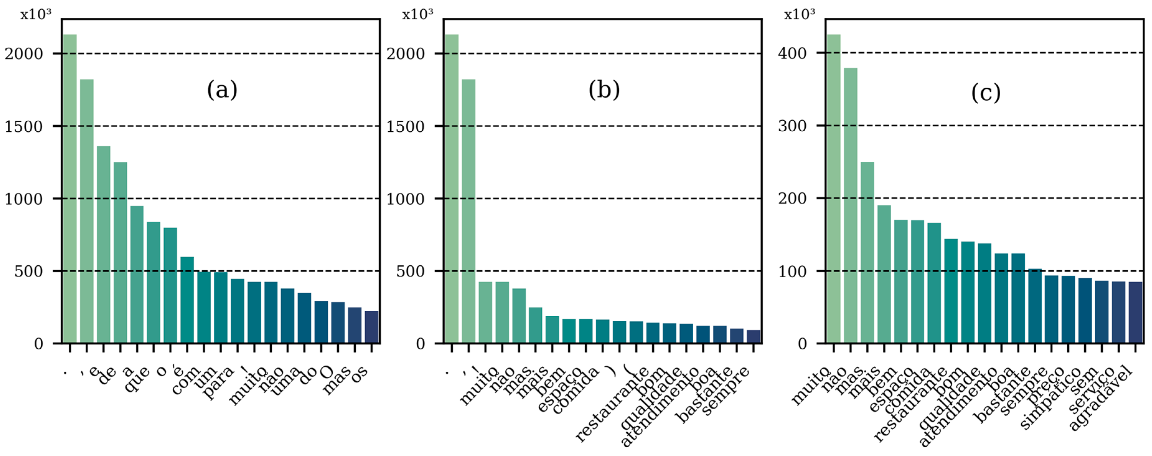
This section introduces the relevant elements to reproduce this study, and the foundations to the decisions made to define the model architecture and the optimization space. The optimization of the hyperparameters and architectural choices of the model used in this study can be approached through various techniques. Alternatives include methods such as Bayesian optimization and reinforcement learning (where an agent learns an optimal policy for selecting configurations). While these methods offer distinct advantages, a GA was selected for this research due to its demonstrated efficacy in large, complex, and potentially non-differentiable search spaces often encountered in neural architecture searches [31]. Furthermore, GAs are well-suited for handling a mix of discrete and continuous parameters, although the focus of this study was primarily on discrete architectural choices. Their population-based approach also allows for the parallel exploration of diverse solutions, reducing the risk of premature convergence to local optima and increasing the likelihood of identifying robust model configurations.

2.1. Dataset

The dataset consists of 536,833 Portuguese restaurant text reviews from Zomato Portugal, now known as Dig-In, gathered from 1 April 2014 to 2 September 2022. Each review has a star rating assigned by the same consumer who wrote it. The ratings represent how good the restaurant experience was in terms of five stars (1.0 to 5.0 in increments of 0.5). An exploratory data analysis was conducted to understand the characteristics of the corpus and the distribution of the ratings provided by the users. The dataset was made available to allow the reproducibility of this work in the digital object identifier 10.17632/448d7kts3k.1 [32].

Table 1. Document length and vocabulary size (1-g) from datasets [16] compared with Zomato dataset.

Dataset	Mean Length	Median Length	Vocabulary Size (1 g)
Olist	7	6	3272
Buscape	25	17	13,470
B2W	14	10	12,758
UTLCApps	21	10	28,283
UTLCMovies	15	7	69,711
Used dataset (Zomato Portugal)	73	52	52,388

summarizes relevant statistics from the used dataset, including similar datasets typically used for SA models in the Portuguese language from Brazil [16]. The mean and median length of the reviews were counted considering 1-g tokens and maintaining punctuation marks (each single punctuation mark is considered a token). The vocabulary size was computed considering only the tokens that appear more than five times in the corpus. Additionally, the percentages of tokens representing punctuation marks and stopwords are 13% and 36.3%, respectively, which provide a more concise view of how each review is constituted. The length of Zomato’s reviews is considerably larger than the reviews used in previous studies, which makes it harder to compare the performance of different models among similar studies.

Figure 1 shows how the distribution of Zomato Portugal’s words has an exponential tendency. In Figure 1a, the most frequent tokens belong to the group that may not convey significant information for SA tasks. These tokens represent punctuation marks and stopwords and are typically eliminated for most NLP tasks. Figure 1b,c show how the token distribution changes according to the stopwords and punctuation marks, respectively, arising with more semantically useful words as the top frequent words. Together, stopwords and punctuation marks represent, on average, 58.3% of the total tokens in a review.

The star ratings enable the usage of supervised learning. It is common in the literature to split the star ratings into two (positive and negative) or three (positive, negative, and neutral) categories to provide labels for SA models [16,33]. Dos Santos and Ladeira [19] conducted an empirical foundation for this heuristic, applying a t-Student test to verify the comparability of the star rating with a manual classification performed by a human. The result indicated that the star rating is equivalent to the manual classification, allowing reliable usage for training an ML algorithm.

The rating distribution of the dataset is depicted in

Table 2. Ratings distribution and corresponding sentiment polarity label and imbalance ratio, with corresponding classes.

Labels	1 *	1.5 *	2 *	2.5 *	3 *	3.5 *	4 *	4.5 *	5 *
Star rating (%)	4.3	0.7	3.5	2.0	10.6	10.2	29.7	12.5	26.6
Polarity (%)	8.47			22.76			68.77
Imbalance ratio	1:8			1:3			1:1
Class	Negative			Neutral			Positive

, where most reviews are labeled with more than two and a half stars. The imbalance in the rating is evident, revealing a highly biased distribution toward more stars. Half-star ratings are generally used less by consumers. The ratio between the majority (4 stars) and minority (1.5 stars) groups is significantly large, while the practical difference between, for instance, reviews with 1 and 1.5 stars is hard to tell. The nine original ratings were divided into three groups, whereby 1.0 to 2.0 stars were assigned to the negative class (label 0), 2.5 to 3.5 stars to the neutral class (label 1), and 4.0 to 5.0 stars to the positive class.

2.2. Evaluaton

The procedure used to train and evaluate model candidates during and after the optimization process was to use a cross-validation scheme adopting training and testing sets for each iteration. Additionally, a fraction of the training set is used to assess whether the model is learning. The variation of the training and validation sets may impact on the capacity to evaluate the model robustly. Therefore, this approach provides more stable results. A two-fold cross-validation (TFCV) scheme was used during the optimization procedure, as a longer validation process would have been considerably time-consuming, and a five-fold cross-validation (FFCV) scheme was used to retrieve the performance of the final optimized models. On each fold iteration of the TFCV, 50% of the data are used for training, 30% for testing, and 20% for validation. On the other hand, during FFCV, the ratios are 60%, 20%, and 20%, respectively.

The performance metrics adopted were the accuracy, recall, precision, and area under the receiver operating characteristic curve (ROC-AUC), computed using a ‘one vs. rest’ (OVR) approach. To avoid any dependency on the distribution of the training set, the metrics were computed as the macro average across the three classes. The metrics are expressed as a function of the terms of the confusion matrices of each class. For a single model, the performance of all folds is averaged. Additionally, the F1-score is another relevant metric in the literature, which is computed as the harmonic average between precision and recall.

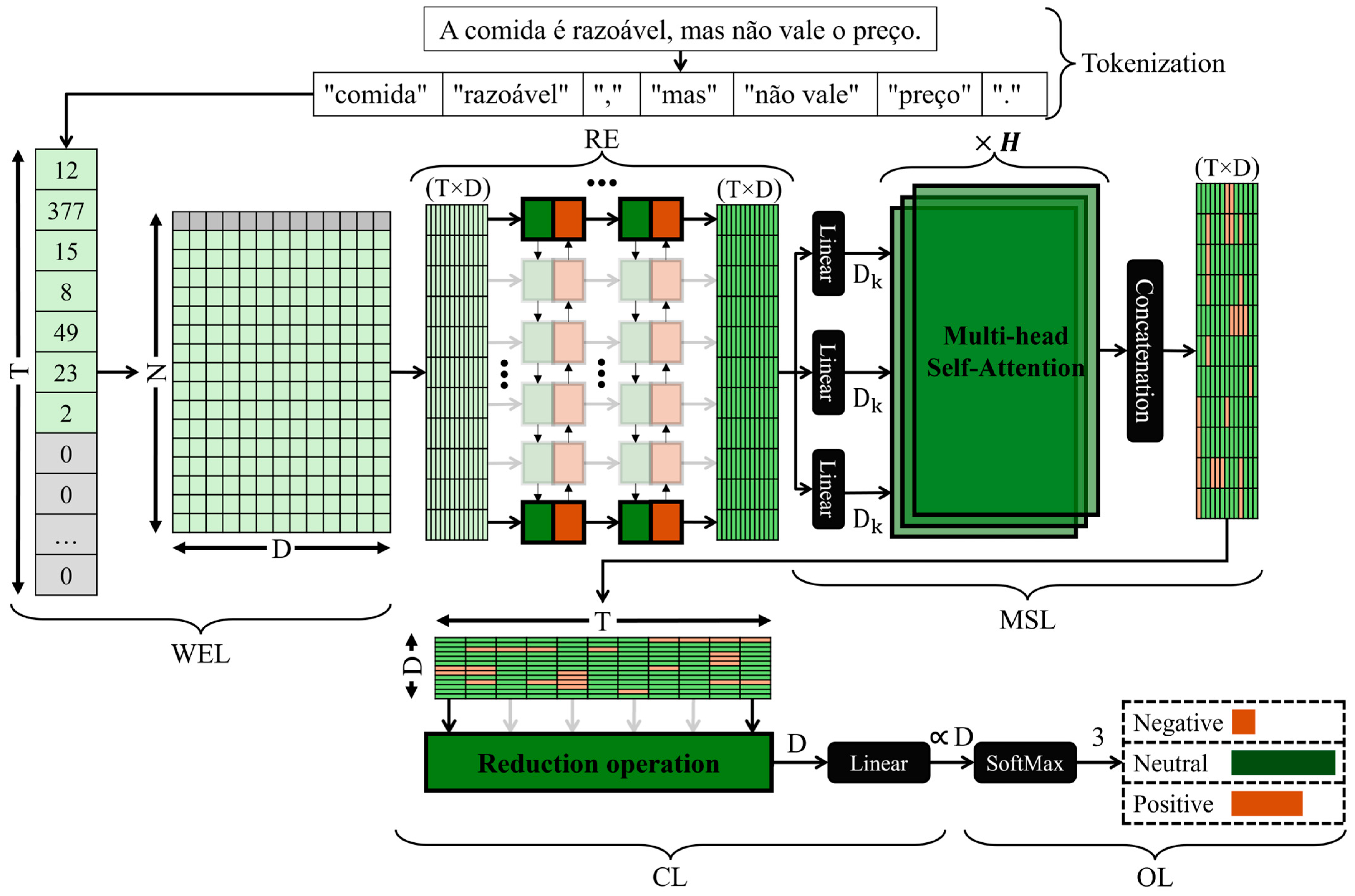
2.3. Model Architecture

The model architecture is intended to be composed of an input word embedding layer, an encoder to extract contextualized information, and an ANN to perform the classification into the three classes. Figure 2 illustrates the general architecture that will be developed. At the input, the text data are tokenized to be digested by the model. This is done using either the Blankspace or Wordpiece tokenizer. The architecture described below is mostly inspired by models found in the literature [16,29,34], disregarding the use of CNN layers and using the Word2Vec algorithm to initialize the embedding weights:

• Word embedding layer (WEL): the input matrix has the dimension $N\times D$, where $N$ is the vocabulary size and $D$ is the number of intended features. This is the interface that transforms the tokenized text into a primary vector representation. The input layer receives a tensor of dimension $T$, which is the pre-defined maximum number of tokens, where each position, or timestep, is an integer that represents a unique token from the vocabulary. Internally, each integer is converted into a one-hot encoding representation and multiplied by the embedding matrix. The vocabulary size was determined heuristically using a quick search algorithm, where a baseline model was trained multiple times, testing values from 5000 to 30,000 tokens. The performance parameter was the ROC-AUC. The resultant vocabulary size was $N$ = 11,560.
  The $D$ features for each $N$ dimension are learned using Word2Vec, an unsupervised neural network algorithm used to extract contextual relationships between adjacent tokens by considering a window of four tokens to each side of the target token, five training epochs, and an initial learning rate of 0.03 to learn $D$ features. Additionally, position embedding is included to identify the position of each token in the input sequence. This is required since the self-attention mechanism does not operate sequentially over tokens. These features are pre-trained and are fine-tuned during the globally supervised training.
• Recurrent encoder (RE): $R$ stacked bidirectional LSTM layers are employed to extract sequential and contextualized information, with $D$ recurrent units each. Additionally, each LSTM layer features a dropout value (in percentage) to avoid overfitting. Unidirectional LSTM layers are also considered for further optimization. Adding multiple layers possibly allows for a more complex model that could learn more intricate relations between the input and output data. For this reason, testing multiple stacked layers is valuable to consider during optimization.
• Multi-head self-attention layer (MSL): This layer emphasizes the most relevant tokens from the input. It is relevant to determine the best position to apply the self-attention mechanism—before, after, or before and after the recurrent encoder. The multi-head self-attention layer is parametrized with $H$ attention heads and an internal projection of $D_k$, given by

  $$D_k=D/H,$$

  (1)

  with an activation function to introduce non-linearities during the computation of the weights. The recurrent encoder and the multi-head self-attention layer constitute the encoder block.
• Classification layer (CL): Once the context vector is produced by the previous layers, an operation is performed to extract and reduce the information that will be passed to the output layer, followed by an ANN with a number of parameters as a function of $D$ and an activation function.
• Output layer (OL): The decoded representation enters a linear layer with three neurons, one for each class. This layer employs a SoftMax activation function to convert the output of the real values into a probability distribution, where the position of the higher value indicates whether the input text is negative, neutral, or positive.

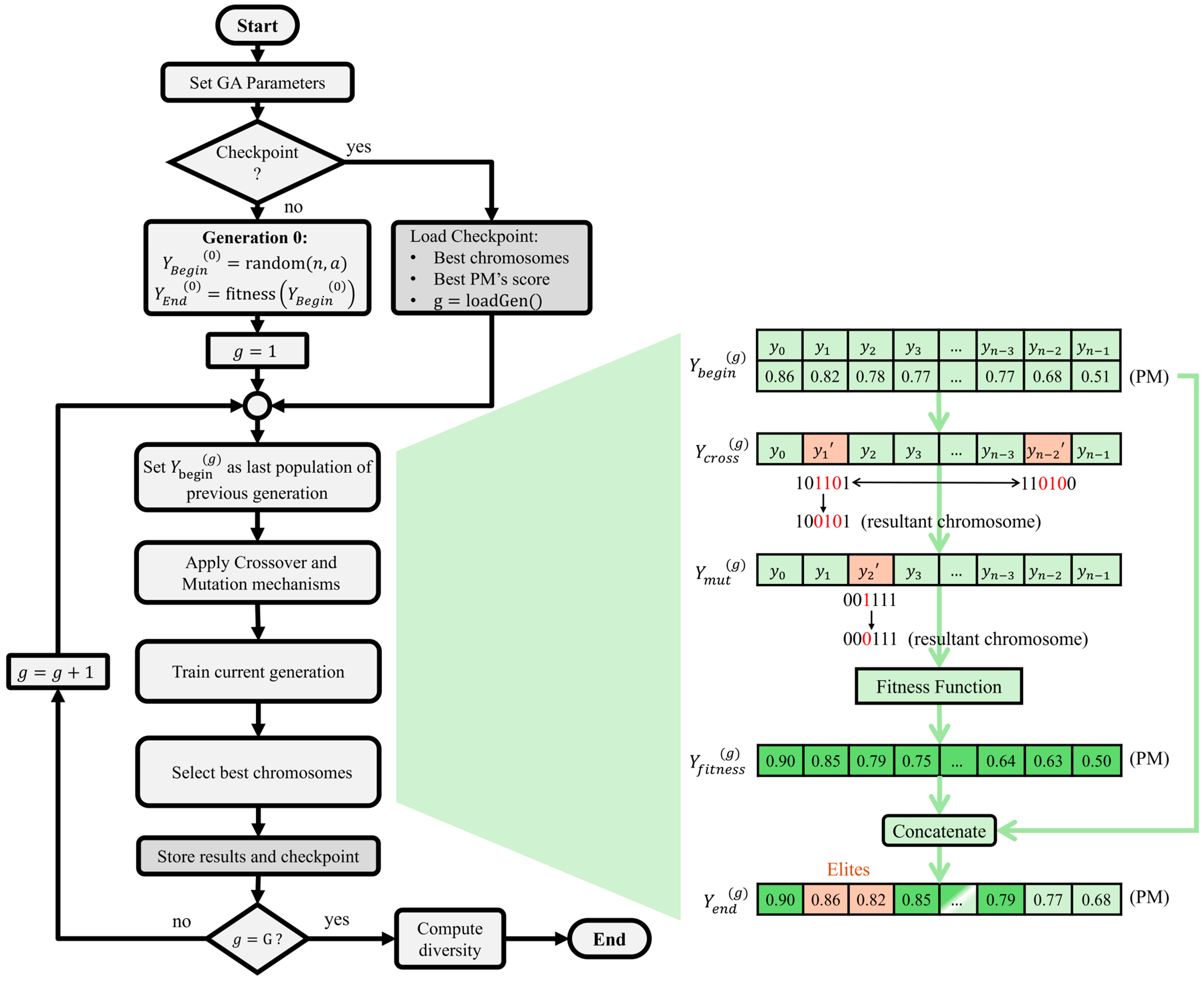
2.4. Genetic Algorithm

The large number of hyperparameters and the wide range of different architectural configurations that the DL model can have motivated the usage of algorithms that automatically search for an optimized model configuration. A GA is a metaheuristic search algorithm that considers the principle of ‘survival of the fittest’. Population-based metaheuristics utilize multiple candidate solutions during the search process. These metaheuristics maintain the diversity in the population and avoid solutions being stuck at a local minimum [31]. This choice was informed by the nature of the hyperparameters targeted for optimization within the LSTM self-attention architecture, which primarily involved discrete variables such as the number of neurons in the LSTM layers, the number of attention heads, or the selection of specific activation functions. Thus, a discrete GA allows for a direct representation and the manipulation of these architectural options. However, the selection of a discrete GA involves trade-offs. Specifically, a continuous GA could incorporate adaptive mechanisms to provide finer-grained control and potentially faster convergence for problems with continuous search spaces or those with dynamic parameter adjustments. On the other hand, a discrete GA provides clarity and simplicity when dealing with inherently categorical or integer-based hyperparameters. For this study, the objective was to effectively explore different structural configurations of the neural network; thus, the discrete GA provided a framework for this combinatorial exploration, proving effective in identifying high-performing architectures for Portuguese sentiment analyses without necessitating the additional complexity that might be introduced by continuous or highly adaptive variants for the specific parameter types under consideration.

While the grid search explores numerous combinations, it might overlook the most significant ones, as its effectiveness relies on the user’s prior knowledge. This algorithm might not be recommended if the defined search space is too broad. On the other hand, the random search finds better models, although this is not guaranteed, requiring less time. When the search space involves numerous hyperparameters, evolutionary algorithms are preferred as they provide guidance in selecting vectors within the search space, as opposed to being entirely random. Although these algorithms take longer to execute, they can be fine-tuned to exert some control over their direction to a certain extent [35,36]. Unlike brute force search algorithms, a GA is not guaranteed to find the best solution. Although it would find a suitable solution, the score might not be optimal.

Figure 3 illustrates the flowchart of the GA. The algorithm was adapted from Mendonça et al. [37], meaning that the expected number of generations, number of parents, length of the chromosomes, mutation rate, and crossover rate were derived from their work. At each iteration, a new generation, $g$, emerges, composed of an initial population that suffers four transformations:

$$Y_{begin}^g=\left\{\begin{array}{l}\mathrm{random}\left(n,a\right),g=0\\ Y_{end}^{g-1},g>0\end{array}\right.,$$

(2)

$${\mathrm{Y}}_{\mathrm{c}\mathrm{r}\mathrm{o}\mathrm{s}\mathrm{s}}^g=\mathrm{c}\mathrm{r}\mathrm{o}\mathrm{s}\mathrm{s}\mathrm{o}\mathrm{v}\mathrm{e}\mathrm{r}\left(Y_{begin}^g,P_{cross}\right),$$

(3)

$${\mathrm{Y}}_{\mathrm{m}\mathrm{u}\mathrm{t}}^g=\mathrm{m}\mathrm{u}\mathrm{t}\mathrm{a}\mathrm{t}\mathrm{i}\mathrm{o}\mathrm{n}(Y_{cross}^g,P_{mut}),$$

(4)

$${\mathrm{Y}}_{\mathrm{f}\mathrm{i}\mathrm{t}\mathrm{n}\mathrm{e}\mathrm{s}\mathrm{s}}^g=\mathrm{f}\mathrm{i}\mathrm{t}\mathrm{n}\mathrm{e}\mathrm{s}\mathrm{s}\left({\mathrm{Y}}_{\mathrm{m}\mathrm{u}\mathrm{t}}^g\right),$$

(5)

$${\mathrm{Y}}_{end}^g=\mathrm{s}\mathrm{e}\mathrm{l}\mathrm{e}\mathrm{c}\mathrm{t}\mathrm{i}\mathrm{o}\mathrm{n}\left({\mathrm{Y}}_{\mathrm{f}\mathrm{i}\mathrm{t}\mathrm{n}\mathrm{e}\mathrm{s}\mathrm{s}}^g,N_{elit}\right),$$

(6)

where each population $Y$ is made of $n$ chromosomes, and each one is composed of a string of $a$ bits that encode information regarding architectural and functional characteristics. The initial population (from generation zero) is an essential factor, responsible for the performance of the GA, its computation time, and the quality of its solutions [31]. The fitness function is the driving force of the GA. Each chromosome is characterized by the value of its performance metric (PM), which in this case is the ROC-AUC determined during the fitness function, where the model is evaluated against a test dataset, using a TFCV scheme. During each generation, except generation zero, the following operations are applied to maintain the diversity:

• Segment crossover operation, with a probability of $P_{cross}$, after $m$ tournaments between two parents. The crossover combines the genetic information of two parents, combining a section of one chromosome into another from the same population. This is an easy-to-implement solution at the cost of less diverse populations. The pseudocode is displayed below.

  Crossover
  Input:	selected_population crossover_rate
  Output:	crossovered_population
  Repeat “size of selected_population” times:    If Apply crossover(crossover_rate)?      parent1 = select_random_chromosome()      parent2 = select_random_chromosome()      assert parent1 != parent2          point1, point2 = select_random_bits_in_chromosome()      new_child <-- parent1      new_child[point1:point2] <-- parent2[point1:point2]    Else      parent = select_random_chromosome()      new_child <-- parent    End If    Add_to_population(crossovered_population, new_child)

• Bit flipping mutation operation, with a probability of $P_{mut}$, with a decreasing mutation rate along the generations. The mutations maintain genetic diversity from one population to the next one.

  Mutation
  Input:	crossovered_population mutation_rate current_gen
  Output:	mutated_population new_mutation_rate
  $\mathrm{n}\mathrm{e}\mathrm{w}\_\mathrm{m}\mathrm{u}\mathrm{t}\mathrm{a}\mathrm{t}\mathrm{i}\mathrm{o}\mathrm{n}\_\mathrm{r}\mathrm{a}\mathrm{t}\mathrm{e}=\max \left(\mathrm{m}\mathrm{u}\mathrm{t}\mathrm{a}\mathrm{t}\mathrm{i}\mathrm{o}\mathrm{n}\_\mathrm{r}\mathrm{a}\mathrm{t}\mathrm{e}\times \left(1-⌊{\displaystyle \frac{\mathrm{c}\mathrm{u}\mathrm{r}\mathrm{r}\mathrm{e}\mathrm{n}\mathrm{t}\_\mathrm{g}\mathrm{e}\mathrm{n}}{5}}⌋\times 30\%\right),0.01\right)$
  For each chromosome in crossovered_population    For each bit in chromosome     If Apply mutation(new_mutation_rate)      New_chromosome[bit] = NOT(chromosome[bit])     Else      New_chromosome[bit] = chromosome[bit]     End If    Add_to_population(mutated_population, New_chromosome)

• Rank selection between parents and children, based on the PM, always maintaining the $N_{elit}$ most fitted chromosomes from $Y_{begin}^g$ to the next generation (elitism), while keeping $n$ constant. The convergence rate of the GA depends upon the selection pressure, and employing elitism reduces the chances of premature convergence.

  Rank selection
  Input:	parents_population children_population
  Output:	selected_population
  Note: parents_population and children_population are sorted by score (AUC) 1. Group Parents and Children (leaving empty locations for Elite chromosomes). 2. Sort group of Parents and Children (best ones are first). 3. Select Elite members and place them in the top of the new population. 4. Sort the selected_population by score (best ones are first).

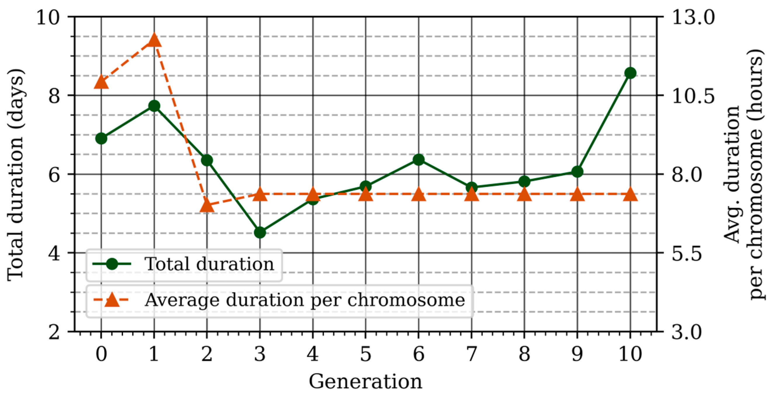
The GA saves data from each generation to allow it to restart from a checkpoint for continuing the optimization. When the GA stops, the diversity is computed for each ${\mathrm{Y}}_{end}^g$ population to assess how different the chromosomes are within each population. The diversity of a generation, $g$, is given by [37]

$$Div\left(g\right)={\displaystyle \frac{2}{zL(z-1)}}{\sum }_{\mu =1}^{z-1}{\sum }_{\theta =\mu +1}^z\mathrm{H}\mathrm{a}\mathrm{m}(p_{\mu },p_{\theta }),$$

(7)

where $L$ is the length of the chromosome, $z$ is the number of chromosomes in the population, and Ham is the Hamming distance given by the number of positions where the bits of the two chromosomes differ.

2.4.1. Training

The fitness function is computed for each population, using a TFCV scheme for evaluation. Therefore, for each $Y$ population, the fitness function trains $n$ architectures twice and evaluates its performance on the test set for each training session, then averages the results. The preliminary experimentation showed that each model takes an average of 2.5 h to train and be tested. Hence, each architecture may take an average of 5 h. Note that this is an approximation and might vary depending on how big the architecture is under the test results.

The training was performed on an NVIDIA GeForce RTX 3090 GPU with a dedicated memory capacity of 24 GB. The framework used to develop the models was TensorFlow 2.9.1 in Python 3, alongside Keras. The batch size was set to 128, which was the maximum value the GPU could use with these models. The RMSprop algorithm was used to update the models’ parameters, typically preferred for LSTM layers, with a learning rate of 0.0001. The categorical cross-entropy function was defined as the loss function for the three output classes, with the label smoothing parameter set to 0.05 to regularize the training.

Two callback functions were used during training: a learning rate scheduler to ensure a warmup interval of three epochs, followed by an exponential learning rate decay; an early stopping mechanism that monitors the ROC-AUC on the validation set, with a minimum detectable variation of 0.0005 and a patience of 30 epochs. If the early stopping mechanism is not triggered, the model trains up to 100 epochs. Finally, in an attempt to overcome the effect of the data imbalance seen in Section 2.1, fixed penalty weights were applied to each class during the computation of the loss function, allowing the impact that the cost function has in the gradient based on the class that is being misclassified to be changed. This is referred to as cost-sensitive learning (CSL). The minority classes have a more significant impact on the gradient when misclassified, while the majority have less impact. These weights were defined using the inverse of each class’s frequency in the training dataset.

2.4.2. Parametrization

The GA was parametrized with a population of $n=15$ chromosomes per generation. Each chromosome is composed of $a=21$ bits, randomly initialized at the beginning of the algorithm. The GA uses an early stopping criterion; if no improvement is observed for three consecutive generations, the algorithm is terminated.

The mutation rate is $P_{mut}=0.2$, with a decreasing rate of 1.2% per generation and limited to a minimum of 1.0%. The crossover rate was defined to $P_{cross}=0.9$ to allow considerable variation of the population. Lastly, when selecting the population for the next generation, we considered $N_{elit}=2$ elite individuals from the parent’s population to pass on to the next generation.

2.4.3. Search Space

A binary string was designed based on heuristics to encode architectural and functional modifications.

Table 3. Definition of the discrete optimization search space for the GA. Each feature is characterized by one to three loci.

Hyperparameter	Locus	Definition
Direction of LSTM layers	0	0: Unidirectional	1: Bidirectional
Number of stacked LSTM layers	1–2	00: 1 10: 3	01: 2 11: 4
Position of self-attention layer	3–4	00: No 10: After	01: Before 11: Both
Model dimension	5–6	00: 300 10: 768	01: 512 11: 1024
Heads dimension	7–8	00: 32 10: 128	01: 64 11: 256
Dropout percentage	9–11	000: 5 100: 25 001: 10 101: 30	010: 15 110: 35 011: 20 111: 40
Operation before classification layer	12–13	00: FFNN 10: LSTM	01: Pooling 11: BiLSTM
Classification layer shape factor	14–15	00: 0.0 10: 1.0	01: 0.5 11: 1.5
Activation function	16–17	00: ReLU 10: Leaky-ReLU	01: Tanh 11: eLU
Encoder replications	18–19	00: 0 10: 2	01: 1 11: 3
Tokenizer	20	0: Blankspace	1: WordPiece

describes the 21 bits used to characterize each chromosome of the population.

The self-attention layers can be placed either before, after, or before and after the stacked LSTM layers, always being applied over the dimension of the tokens. Additionally, the option of removing attention mechanisms was also considered. The dimensionality of the model was defined as values in powers of two, except for the value 300, which is a typical value in the literature. The dimensionality of the head’s projection was defined ensuring that the resulting number of heads was an integer value. When the particular case of $D=300$ occurs, then the $D_k$ value is converted to the nearest integer multiple of 300. Different operations for the classification layer were considered by intuition, for which average pooling and recurrent mechanisms have already been used in the literature [29,38]. Loci 18 and 19 give the possibility of replicating the encoder block one to three times, potentially allowing the model to extract more semantic features. When the encoder block is replicated, the output of each attention layer is normalized with residual connections from the input of the prior layer, like the transformer.

The developed codebase is available at www.github.com/danidoliv66/Optimizing-LSTMSA-PTSA-GenAlg (accessed on 30 May 2025).

3. Results

The GA took about 70 days (approximately 5 h to train and evaluate a single model architecture) to complete the eleven generations (ten generations plus generation zero). The optimization process is a considerably slow process, as shown in Figure 4. However, as the generations advance, the population converges into more stable architectures, causing the populations of the last generations to be trained about 1.6 times faster.

Figure 5 shows how the PM of the best chromosome increases along with the generations sideways with the reduction in diversity for the new generations. The best chromosome emerged in the seventh generation, while in the eighth, it registered an increase in diversity, which suggests there is potential for further optimization, as unseen architectures may now be explored. At the last fitted generation, the PM remained the same; therefore, the previous best chromosome was considered an elite member of the population.

In addition to selecting the best architecture for the neural network, the intermediate architectures can be analyzed to find which patterns were beneficial for training the model. This is discussed in the following subsections.

Furthermore, the best architecture is compared to the models found in the literature, with emphasis on the baseline model from Branco et al. [27], referred to as BaseModel, which is the BERTimbau model retrained with transfer learning with the same dataset from this work [32].

Each generation continuously converges into a set of the most desirable features. These features are the ones that allow the best fitness in the training environment and the characteristics of the dataset. Understanding the most important features of the latest populations enables one to disregard the hyperparameters or architectural characteristics that do not fit the dataset while providing insights into which hyperparameters the GA should focus on the most. Potentially, the top five provide the most significant information about each generation.

Figure 6 reveals the evolution of each generation in time in terms of the LSTM and self-attention layers. As the number of generations increases, the overall number of LSTM layers tends to be reduced. Bidirectionality is preferred in later generations, although the number of unidirectional layers is larger for the top five chromosomes, due to chromosomes that replicate the encoder several times and increase their complexity. On the other hand, the unidirectional LSTM layer is more prevalent in the decoder block of the architecture after generation four. Regarding the self-attention layers, there was a peak in generation three that indicates a temporal tendency, which was replaced by a new tendency in the next generation. In generation three, several replications of the encoder block were very common but they were rapidly reduced. The number of self-attention layers before the recurrent decoder started dropping from generation three, while the number of self-attention layers after the LSTM layers became the norm in later generations.

The dimensionality of the architecture is of great concern, as it decides the number of trainable parameters of the model. Figure 7 shows the preferred dimensionality over the last three generations of the GA, regarding only the top five chromosomes from each, revealing that $D=1024$ is the most common size among the populations, with 32 attention heads of 32 dimensions each. The output neural network ended up disappearing from the model’s architecture. Moreover, the best chromosome from the last generation features all of these design trend characteristics.

In the last generations, the eLU activation layer and the WordPiece tokenizer disappeared. This is a relevant result, as it makes it possible to disregard these features for future models. On the other hand, the ReLU and TanH activation functions were the most common cases. Typical dropout percentages are below 20%. The encoder block is normally replicated less than twice, as more replications lead to bigger models that may not have sufficient data to learn language relationships. In addition, the most common is to be replicated once (two encoder blocks), possibly because it is the simpler architecture that includes normalization and residual connections, which greatly improve the performance during training.

Based on the previous analysis, the best architecture was considered to be the best chromosome from the seventh population (Figure 5). The best chromosomes typically feature Bi-LSTM layers followed by self-attention mechanisms, where this block is replicated twice. The final model architecture was trained from scratch under similar conditions to extract more information about its sensitivity and precision, as well as its overall accuracy, employing the FFCV.

Figure 8 compares the accuracy, recall, precision, and ROC-AUC of the newer architecture against the BaseModel [27]. The increases in the ROC-AUC and the accuracy are notable, which indicate that the model correctly classified more instances. On the other hand, the decreases in precision and recall suggest that the F1-score decreased, mainly due to its precision. This reduction implies that the model became less conservative in predicting the minority classes (negative and neutral), resulting in more false positives but fewer false negatives. This is beneficial, in this case, due to the data imbalance scenario, where the positive class is overrepresented. Only the class weights in the loss function were beneficial for partially surpassing the bias from class skewness. The difference in the number of trainable parameters between the BaseModel and the optimized architecture is a decrease of approximately 2.7 times.

In addition to the average metrics, the micro- (per class) metrics of the ROC-AUC and F1-score can be analyzed to understand how the data imbalance affects the model behavior on each class. The ROC-AUC values of the negative and positive classes are 89.6% and 83.9%, respectively, indicating the model has a greater affinity for the negative class, which is desirable since the majority class is the positive, and training tends to be biased towards this class. On the other hand, the F1-scores of the negative and positive classes are 75.8% and 89.2%, respectively, indicating that the model is still biased to the positive class. This opposed behavior illustrates the trade-off. The high ROC-AUC on the negative class, despite the class imbalance, provokes an increase in false positives on the negative class, reducing the F1-score of the negative class. Furthermore, inspecting the confusion matrix of Figure 9, the most difficult class to classify is the neutral class, causing an increased number of false positives and false negatives for that class. The false positives of the positive class equal 26.8% due to the class imbalance, as the neutral class is commonly misclassified as positive. Finally, the confusion matrix shows that the model is very effective at differentiating between positive and negative.

4. Discussion

Table 4. Comparison of models developed in previous studies. The accuracy and F1-score are considered the performance metrics, as these are the most common in the literature.

Reference	Model	Accuracy	F1-Score
Brum and Nunes, 2017 [17]	NB	64.6	59.9
Gomes et al., 2018 [18]	LR	81.3	79.6
Adán-Coello and Neto, 2019 [25]	Self-AT-LSTM	66.5	67.6
Britto et al., 2022 [26]	BERTimbau	78.8	66.8
Branco et al., 2024 [27]	BERTimbau with AdaBoost	84.0	77.7
This study	LSTM-SA	81.5	75.4

provides a summary of the results of previous studies of SA models with the positive, negative, and neutral classes, compared with the model that resulted in this study after the GA optimization. The first two models refer to classic ML approaches, while the last three refer to DL approaches. Finally, the last model refers to the architecture found in this study, revealing an apparent improvement from previous studies. The actual performance might be hinged by the particularities of the dataset used in each study, namely the data imbalance and the domain of the reviews. The results from Xia et al. [29] were included despite being from an English dataset because the architecture developed in this study was greatly based on theirs. Brum and Nunes [17] used the TweetSentBR dataset, dos Santos and Ladeira [19] scrapped the reviews available in the Google Play app store, and Britto et al. [26] used the datasets compiled by Souza and Souza Filho [16]. Branco et al. [27] used the same dataset used in this study; therefore, it was the most relevant for comparison.

Regarding the number of trainable parameters, the BERTimbau model trained with AdaBoost [27] provided the greatest performance with the same dataset, with a total of 220 million parameters. The model from this study is approximately five times smaller (41.1 million parameters), with an absolute loss in performance of 2.5% in accuracy and 2.3% in F1-score when compared to theirs. Therefore, the optimization process was valuable to increase the performance of the model while maintaining a relatively small number of trainable parameters, and provides better performance than in previous studies, including when compared to the BERTimbau model trained solely with transfer learning. Furthermore, the optimization could not surpass the performance of more complex training techniques such as boosting [27].

The GA was used to fine-tune the model’s hyperparameters and identify optimal configurations, demonstrating effective optimization. This process can be time-consuming, and the improvements might sometimes be very subtle. The GA was stopped at the eighth generation when the PM had increased sufficiently and was also limited by time availability. Further generations might have potentially increased model performance, as depicted by the increase in diversity.

Regarding the first research question, the results showed a viable level of performance, helped not only by the optimization process but also by the training configuration, namely the usage of the CSL scheme. The usage of LLMs may provide superior performance [27] but at the cost of a large number of parameters (five times bigger for a gain of 2.5% in accuracy). The possibility to develop comparable models with less computational costs provides more feasibility for lower-resource environments. This shows that the optimization of simpler models can lead to considerable gains in performance for the same problem, i.e., the Zomato Portugal dataset.

For the second research question, the GA proved to provide significant improvements in the baseline and the best chromosome, which will depend on the available time for optimization and the quality of the search space. The greater limitation of discrete GAs is the manual definition of the optimization space, which may lead to bias or hinge optimal configurations. Notably, the large number of architectural changes found by the GA is relevant, indicating that self-attention models are more sensitive to their parametrization, especially the number of parameters. During the optimization, it was possible to find models up to approximately 200 million parameters, which take longer to train and typically do not gain enough in performance, possibly due to the lack of data.

However, it is relevant to note that the comparison between similar studies is not robust, as the training datasets are fairly different and the usage of the ROC-AUC as the PM is not widely adopted yet in all related papers.

5. Conclusions

This research demonstrated the utility of employing a GA for the optimization of an LSTM self-attention architecture specifically applied to Portuguese sentiment analyses. The study’s findings show that GAs provide an effective method for optimizing the complex hyperparameter space inherent in advanced deep learning models. This conclusion is particularly relevant for languages such as Portuguese, where the availability of extensively pre-tuned models or deep-language-specific NLP expertise may be less developed compared to high-resource languages. The GA-driven optimization process can identify effective architectural configurations that might otherwise require extensive manual tuning, thereby providing a more systematic approach to model development.

The practical implications of this research extend to NLP tasks for minority or lesser-resourced languages. Specifically, the automation provided by GA optimization can lessen the human efforts and computational resources often associated with adapting and fine-tuning complex neural network models for new linguistic contexts. This can facilitate the achievement of robust results in settings with limited resource availability. Furthermore, as the GA explores a range of architectural parameters, it can then assist in developing models that better address the specific linguistic characteristics and nuances of a given minority language. Such an approach supports the development of NLP tools suitable for particular languages, rather than relying solely on the adaptation of models primarily trained on different linguistic structures. This work, therefore, contributes a methodological framework that can be considered for SA and other NLP tasks in various minority languages, potentially aiding in the creation of effective, language-specific NLP applications. Future investigations could focus on applying this methodology to other less-resourced languages and examining the transferability of the optimized architecture to other languages.

There is also a need to address several aspects of the optimization procedure in the future to improve the performance of the neural network model for SA tasks. A potential method of exploration is to assess the scalability of the models to include the concatenation of 100-token chunks for sequential evaluation, followed by the usage of pooling layers or a weighted voting mechanism to aggregate the input sequences. Alternatively, it is possible to retrain the network while providing access to the recurrent encoder’s initial and last hidden and cell states. In this way, information about the previous 100-token chunk can be provided without significantly changing the network architecture. Additionally, dimension reduction algorithms can be employed on initial embeddings to obtain a fixed-size representation, disregarding the initial and variable numbers of tokens. This requires the model’s input to the altered to allow a customized initialization of the hidden state.

This research was limited to LSTMs and self-attention mechanisms. Thus, future work might explore other configurations, such as combining CNNs and LSTMs for feature extraction and other attention mechanisms for encoding. Furthermore, it is important to prioritize the model’s explainability in future research, as it remains a black box. Additionally, the next research step is to perform SA tasks at a deeper level of granularity, exploring sentence and aspect levels of classification.

References

1. Zhang, L.; Wang, S.; Liu, B. Deep Learning for Sentiment Analysis: A Survey. WIREs Data Min. Knowl. Discov. 2018, 8, e1253. [Google Scholar] [CrossRef]
2. Young, T.; Hazarika, D.; Poria, S.; Cambria, E. Recent Trends in Deep Learning Based Natural Language Processing [Review Article]. IEEE Comput. Intell. Mag. 2018, 13, 55–75. [Google Scholar] [CrossRef]
3. Khurana, D.; Koli, A.; Khatter, K.; Singh, S. Natural Language Processing: State of The Art, Current Trends and Challenges. Multimed. Tools Appl. 2022, 82, 3713–3744. [Google Scholar] [CrossRef] [PubMed]
4. Touvron, H.; Lavril, T.; Izacard, G.; Martinet, X.; Lachaux, M.A.; Lacroix, T.; Rozière, B.; Goyal, N.; Hambro, E.; Azhar, F.; et al. LLaMA: Open and Efficient Foundation Language Models. arXiv 2023. [Google Scholar] [CrossRef]
5. Languages Most Frequently Used for Web Content as of January 2024, by Share of Websites. Available online: https://www.statista.com/statistics/262946/most-common-languages-on-the-internet/ (accessed on 19 June 2024).
6. Ferrone, L.; Zanzotto, F.M. Symbolic, Distributed and Distributional Representations for Natural Language Processing in the Era of Deep Learning: A Survey. Front. Robot. AI 2020, 6, 153. [Google Scholar] [CrossRef]
7. Otter, D.; Medina, J.; Kalita, J. A Survey of the Usages of Deep Learning for Natural Language Processing. IEEE Trans. Neural Netw. Learn. Syst. 2020, 32, 604–624. [Google Scholar] [CrossRef]
8. Mao, Y.; Liu, Q.; Zhang, Y. Sentiment analysis methods, applications, and challenges: A systematic literature review. J. King Saud Univ. Comput. Inf. Sci. 2024, 36, 102048. [Google Scholar] [CrossRef]
9. Pereira, D.A. A Survey of Sentiment Analysis in the Portuguese Language. Artif. Intell. Rev. 2021, 54, 1087–1115. [Google Scholar] [CrossRef]
10. Devlin, J.; Chang, M.-W.; Lee, K.; Toutanova, K. BERT: Pre-training of Deep Bidirectional Transformers for Language Understanding. In Proceedings of the 2019 Conference of the North American Chapter of the Association for Computational Linguistics: Human Language Technologies (Long and Short Papers), Minneapolis, MN, USA, 2–7 June 2019; Association for Computational Linguistics: Stroudsburg, PA, USA, 2019; pp. 4171–4186. [Google Scholar] [CrossRef]
11. Wankhade, M.; Rao, A.; Kulkarni, C. A survey on sentiment analysis methods, applications, and challenges. Artif. Intell. Rev. 2022, 55, 5731–5780. [Google Scholar] [CrossRef]
12. Rehman, A.U.; Malik, A.K.; Raza, B.; Ali, W. A Hybrid CNN-LSTM Model for Improving Accuracy of Movie Reviews Sentiment Analysis. Multimed. Tools Appl. 2019, 78, 26597–26613. [Google Scholar] [CrossRef]
13. Souza, F.; Nogueira, R.; Lotufo, R. BERTimbau: Pretrained BERT Models for Brazilian Portuguese. In Intelligent Systems; Cerri, R., Prati, R.C., Eds.; Lecture Notes in Computer Science; Springer International Publishing: Cham, Switzerland, 2020; Volume 12319, pp. 403–417. [Google Scholar] [CrossRef]
14. Rodrigues, J.; Gomes, L.; Silva, J.; Branco, A.; Santos, R.; Cardoso, H.L.; Osório, T. Advancing Neural Encoding of Portuguese with Transformer Albertina PT-*. arXiv 2023. [Google Scholar] [CrossRef]
15. Souza, E.; Vitório, D.; Castro, D.; Oliveira, A.L.I.; Gusmão, C. Characterizing Opinion Mining: A Systematic Mapping Study of the Portuguese Language. In Proceedings of Computational Processing of the Portuguese Language, Processings of the 12th International Conference, PROPOR 2016, Tomar, Portugal, 13–15 July 2016; Lecture Notes in Computer Science; Springer International Publishing: Cham, Switzerland, 2016; Volume 9727, pp. 122–127. [Google Scholar] [CrossRef]
16. Souza, F.D.; Baptista de Oliveira e Souza Filho, J. Sentiment Analysis on Brazilian Portuguese User Reviews. In Proceedings of the 2021 IEEE Latin American Conference on Computational Intelligence (LA-CCI), Temuco, Chile, 2–4 November 2021; pp. 1–6. [Google Scholar] [CrossRef]
17. Brum, H.B.; Nunes, M.d.G.V. Building a Sentiment Corpus of Tweets in Brazilian Portuguese. In Proceedings of the Eleventh International Conference on Language Resources and Evaluation (LREC 2018), Miyazaki, Japan, 7–12 May 2018; European Language Resources Association (ELRA): Paris, France, 2017; pp. 4167–4172. [Google Scholar] [CrossRef]
18. Gomes, F.B.; Coello, J.M.A.; Kintschner, F.E. Studying the Effects of Text Preprocessing and Ensemble Methods on Sentiment Analysis of Brazilian Portuguese Tweets. In Statistical Language and Speech Processing, Proceedings of the 6th International Conference, SLSP 2018, Mons, Belgium, 15–16 October 2018; Lecture Notes in Computer Science; Springer Nature Switzerland: Cham, Switzerland, 2018; pp. 167–177. [Google Scholar] [CrossRef]
19. dos Santos, F.L.; Ladeira, M. The Role of Text Pre-processing in Opinion Mining on a Social Media Language Dataset. In Proceedings of the 2014 Brazilian Conference on Intelligent Systems, Sao Paulo, Brazil, 18–22 October 2014; pp. 50–54. [Google Scholar] [CrossRef]
20. Souza, F.D.; Baptista de Oliveira e Souza Filho, J. Embedding Generation for Text Classification of Brazilian Portuguese User Reviews: From Bag-of-Words to Transformers. Neural Comput. Appl. 2022, 35, 9393–9406. [Google Scholar] [CrossRef]
21. Repositório de Word Embeddings do NILC. Available online: http://www.nilc.icmc.usp.br/embeddings (accessed on 30 June 2023).
22. Vianna, D.; Carneiro, F.; Carvalho, J.; Plastino, A.; Paes, A. Sentiment analysis in Portuguese tweets: An evaluation of diverse word representation models. Lang Resour. Eval. 2024, 58, 223–272. [Google Scholar] [CrossRef]
23. Cardoso, M.H.; Maria Da Rocha Fernandes, A.; Marin, G.; Quietinho Leithardt, V.R.; Crocker, P. Comparison between Different Approaches to Sentiment Analysis in the Context of the Portuguese Language. In Proceedings of the 16th Iberian Conference on Information Systems and Technologies (CISTI), Chaves, Portugal, 23–26 June 2021; pp. 1–6. [Google Scholar] [CrossRef]
24. de Oliveira, D.N.; de, C. Merschmann, L.H. Joint Evaluation of Preprocessing Tasks with Classifiers for Sentiment Analysis in Brazilian Portuguese Language. Multimed. Tools Appl. 2021, 80, 15391–15412. [Google Scholar] [CrossRef]
25. Adán-Coello, J.M.; Neto, A.D.C. Sentiment Analysis of Tweets in Brazilian Portuguese with Convolutional Neural Networks. Int. J. Innov. Educ. Res. 2019, 7, 29–41. [Google Scholar] [CrossRef]
26. Britto, L.F.S.; Pessoa, L.A.S.; Agostinho, S.C.C. Cross-Domain Sentiment Analysis in Portuguese using BERT. In Proceedings of the Anais do XIX Encontro Nacional de Inteligência Artificial e Computacional (ENIAC 2022), Campinas, Brazil, 28 November–1 December 2022; Sociedade Brasileira de Computação-SBC: Porto Alegre, Brazil, 2022; pp. 61–72. [Google Scholar] [CrossRef]
27. Branco, A.; Parada, D.; Silva, M.; Mendonça, F.; Mostafa, S.S.; Morgado-Dias, F. Sentiment Analysis in Portuguese Restaurant Reviews: Application of Transformer Models in Edge Computing. Electronics 2024, 13, 589. [Google Scholar] [CrossRef]
28. Vaswani, A.; Shazeer, N.; Parmar, N.; Uszkoreit, J.; Jones, L.; Gomez, A.N.; Kaiser, L.; Polosukhin, I. Attention Is All You Need. arXiv 2017. [Google Scholar] [CrossRef]
29. Xia, H.; Ding, C.; Liu, Y. Sentiment Analysis Model Based on Self-Attention and Character-Level Embedding. IEEE Access 2020, 8, 184614–184620. [Google Scholar] [CrossRef]
30. Wu, Z.; Nguyen, T.-S.; Ong, D. Structured Self-Attention Weights Encode Semantics in Sentiment Analysis. In Proceedings of the Third BlackboxNLP Workshop on Analyzing and Interpreting Neural Networks for NLP, Online, 20 November 2020; Association for Computational Linguistics: Stroudsburg, PA, USA, 2020; pp. 255–264. [Google Scholar] [CrossRef]
31. Katoch, S.; Chauhan, S.S.; Kumar, V. A review on genetic algorithm: Past, present, and future. Multimed. Tools Appl. 2021, 80, 8091–8126. [Google Scholar] [CrossRef]
32. De Olival, D.; Branco, A.; Silva, M.; Mendonça, F.; Mostafa, S.S.; Morgado-Dias, F. PT-EN Zomato Dataset. Mendeley Data 2024. [Google Scholar] [CrossRef]
33. Yadollahi, A.; Shahraki, A.; Zaïane, O. Current State of Text Sentiment Analysis from Opinion to Emotion Mining. ACM Comput. Surv. 2017, 50, 1–33. [Google Scholar] [CrossRef]
34. AL-Smadi, M.; Hammad, M.M.; Al-Zboon, S.A.; AL-Tawalbeh, S.; Cambria, E. Gated Recurrent Unit with Multilingual Universal Sentence Encoder for Arabic Aspect-Based Sentiment Analysis. Knowl.-Based Syst. 2023, 261, 107540. [Google Scholar] [CrossRef]
35. Bergstra, J.; Bengio, Y. Random Search for Hyper-Parameter Optimization. J. Mach. Learn. Res. 2012, 13, 281–305. [Google Scholar] [CrossRef]
36. Liashchynskyi, P.B.; Liashchynskyi, P. Grid Search, Random Search, Genetic Algorithm: A Big Comparison for NAS. arXiv 2019, arXiv:1912.06059v1. [Google Scholar]
37. Mendonça, F.; Mostafa, S.S.; Freitas, D.; Morgado-Dias, F.; Ravelo-García, A.G. Multiple Time Series Fusion Based on LSTM: An Application to CAP A Phase Classification Using EEG. Int. J. Environ. Res. Public Health 2022, 19, 10892. [Google Scholar] [CrossRef]
38. Zhou, P.; Qi, Z.; Zheng, S.; Xu, J.; Bao, H.; Xu, B. Text Classification Improved by Integrating Bidirectional LSTM with Two-dimensional Max Pooling. In Proceedings of the COLING 2016, the 26th International Conference on Computational Linguistics: Technical Papers, Osaka, Japan, 11–16 December 2016; ACL: Stroudsburg, PA, USA, 2016; pp. 3485–3495. Available online: http://dblp.uni-trier.de/db/conf/coling/coling2016.html#ZhouQZXBX16 (accessed on 12 January 2025).
Figure 1. Top 20 most frequent tokens of Zomato Portugal dataset between 1 April 2014 and 2 September 2022: (a) frequency of all tokens; (b) frequency of all tokens after removing the stopwords; (c) frequency of all tokens after removing the stopwords and punctuation marks.
Applsci 15 06336 g001
Figure 2. Proposed model architecture, composed of an input embedding matrix pre-trained with Word2Vec, a recursive encoder, a multi-head self-attention block, a decoder, and an output layer.
Applsci 15 06336 g002
Figure 3. Flowchart of the implemented GA. On the right side there is an example of how the chromosomes and their scores propagate along the chart.
Applsci 15 06336 g003
Figure 4. Durations of the optimization process: total duration (left axis) and average duration per chromosome (right axis).
Applsci 15 06336 g004
Figure 5. Performance of each generation over time, measured by the ROC-AUC score (right axis) and the diversity (left axis) of each population.
Applsci 15 06336 g005
Figure 6. Evolution of the numbers of LSTM layers and self-attention layers over time. ‘All chromosomes show the average of all chromosomes within the generation, while the top 5 chromosomes show how the most relevant chromosomes are built.
Applsci 15 06336 g006
Figure 7. Distribution of the dimensions found during the GA.
Applsci 15 06336 g007
Figure 8. Comparison of the metrics extracted from FFCV of the baseline and the GA architectures [27].
Applsci 15 06336 g008
Figure 9. Confusion matrix of the model optimized by the GA.
Applsci 15 06336 g009