Unsupervised Feature Selection via a Dual-Graph Autoencoder with ${\mathcal{l}}_{\mathbf{2}\mathbf{,}\mathbf{1}\mathbf{/}\mathbf{2}}$-Norm for [⁶⁸Ga]Ga-Pentixafor PET Imaging of Glioma

Featured Application

The proposed unsupervised feature selection method, based on a dual-graph autoencoder, can assist in the automatic characterization of glioma regions from [⁶⁸Ga]Ga-Pentixafor PET/CT images. It has potential applications in clinical decision support systems for tumor delineation, assessment of treatment response, and differentiation between active tumor and necrotic tissue, particularly in patients with high-grade gliomas.

Abstract

In the era of big data, high-dimensional datasets have become increasingly common in fields such as biometrics, computer vision, and medical imaging. While such data contain abundant information, they are often accompanied by substantial noise, high redundancy, and complex intrinsic structures, posing significant challenges for analysis and modeling. To address these issues, unsupervised feature selection has attracted growing interest due to its ability to handle unlabeled, noisy, and unstructured data. This paper proposes a novel unsupervised feature selection algorithm based on a dual-graph autoencoder (DGA), which combines the powerful data reconstruction capability of autoencoders with the structural preservation strengths of graph regularization. Specifically, the algorithm introduces the ${\mathcal{l}}_{2,1/2}$-norm and ${\mathcal{l}}_{2,1}$-norm constraints on the encoder and decoder weight matrices, respectively, to promote feature sparsity and suppress redundancy. Furthermore, an ${\mathcal{l}}_{2,1/2}$-norm loss term is introduced to enhance robustness against noise and outliers. Two separate adjacency graphs are constructed to capture the local geometric relationships among samples and among features, and their corresponding graph regularization terms are embedded in the training process to retain the intrinsic structure of the data. Experiments on multiple benchmark datasets and [⁶⁸Ga]Ga-Pentixafor PET/CT glioma imaging data demonstrate that the proposed DGA significantly improves clustering performance and accurately identifies features associated with lesion regions. From a clinical perspective, DGA facilitates more accurate lesion characterization and biomarker identification in glioma patients, thereby offering potential utility in aiding diagnosis, treatment planning, and personalized prognosis assessment.

1. Introduction

With the rapid advancement of society and the advent of the big data era, both the volume and dimensionality of data have increased exponentially, resulting in a growing demand for efficient data processing and analysis. High-dimensional data, which are widely encountered in fields such as biometrics, computer vision, and medical imaging, provide rich information but also introduce substantial noise and redundancy, making data analysis more challenging. As dimensionality increases, data distribution becomes sparser, the search space expands, computational complexity rises, and the generalization ability of models tends to decline. Feature selection offers an effective solution by identifying a representative subset of features from the original dataset, which not only improves feature quality and reduces computational cost but also mitigates the curse of dimensionality and enhances model performance, all while preserving the intrinsic structure of the data.

Feature selection methods can be divided into supervised [1,2], semi-supervised [3,4], and unsupervised [5] approaches depending on whether the data labels are fully available, partially available, or entirely unavailable. In many real-world applications, labels are often difficult or impossible to obtain, which limits the applicability of supervised and semi-supervised methods. As a result, unsupervised feature selection, which relies on the intrinsic structure of high-dimensional data rather than label information, has gained increasing attention and demonstrated notable advantages in handling unlabeled data effectively.

According to different selection strategies, feature selection methods can be classified into filter, wrapper, and embedded approaches. Filter methods evaluate feature quality using statistical criteria such as information distance, task relevance, and redundancy and select features based on corresponding scores, with typical algorithms including the Laplacian Score [2], maximum variance, trace ratio, and SPEC [3]. These methods are computationally efficient, model-independent, and highly generalizable; however, they often fail to adapt well to specific tasks or datasets [6]. In contrast, wrapper methods, such as varFnMS [7] and UFSACO [8], perform feature selection based on the predictive performance of selected feature subsets using a specific learning model. While they generally achieve better performance than filter methods, their computational cost is significantly higher, particularly for large-scale datasets, due to the need for repeated feature subset searching and evaluation. Embedded methods integrate feature selection directly into the model training process, enabling the simultaneous optimization of feature subsets and learning models. This approach typically offers improved efficiency over wrapper methods and better task-specific adaptation than filter methods. In this study, we focus on embedded unsupervised feature selection methods, which can generally be divided into regression-based and self-representation-based frameworks. The self-representation-based approach assumes that each feature can be reconstructed as a linear combination of related features. For example, Zheng et al. [9] proposed UFS_SP, and Shang et al. [10] introduced NLRL-LE, which employs non-convex constraints and Laplacian embedding for latent representation learning. Similarly, Wang et al. [11] developed MFFS, a method based on matrix factorization that selects a subset of features capable of representing the remaining features via subspace learning. On the other hand, regression-based methods convert the unsupervised selection problem into a supervised paradigm by generating pseudo-labels for the dataset. For instance, SCFS, proposed by Parsa et al. [12], utilizes symmetric non-negative matrix factorization to derive a cluster indicator matrix, then applies regression to optimize the coefficient matrix and identify the most informative features.

As previously discussed, high-dimensional data often exhibit significant noise, redundancy, and complex intrinsic correlations, making direct analysis and modeling in the original data space highly challenging. In response to these issues, increasing attention has been paid to feature selection algorithms that can effectively preserve the inherent structure of the data, as such preservation not only enhances feature selection performance but also improves model interpretability. To address structural preservation, Cai et al. [13] presented MCFS, which combines sparse regression with spectral analysis to retain the local structural information of the original data. Building upon similar principles, Li et al. [14] introduced NDFS, which integrates spectral clustering with feature selection to capture the intrinsic geometric structure. Cai et al. [13] also proposed GNMF, which constructs a nearest-neighbor graph to preserve the manifold structure. Further advancements include Feng and Duarte [15], who incorporated spectral analysis of projected data into an autoencoder framework, enabling the compression of high-dimensional data into a low-dimensional space while maintaining local structure. Similarly, Shang et al. [10] developed SLREO, which combines sparse latent representation with extended OLSDA. This method integrates OLSDA into a non-negative manifold structure to generate pseudo-labels, ensuring both structure preservation and non-negativity of the labels. Despite their effectiveness, these approaches primarily focus on preserving the manifold structure in the data space, often neglecting the structural information embedded in the feature space. To overcome this limitation, researchers have proposed methods that jointly preserve structures in both data and feature spaces. For example, Gu and Zhou [16] introduced DRCC, while Shang et al. [17] presented DNMF; both approaches simultaneously consider the geometric structures of the sample manifold and the feature manifold, leading to more comprehensive structure-aware feature selection.

Furthermore, norm-based constraints are commonly employed on matrices to enhance robustness, suppress noise, and improve the sparsity of the selection matrix. For instance, Zheng et al. [18] presented NSSLFS, which incorporates ${\mathcal{l}}_1$-norm and ${\mathcal{l}}_{2,1}$-norm into the objective functions to achieve sparsity and robustness. Shang et al. [17] applied an ${\mathcal{l}}_{2,1}$-norm constraint to the residual matrix of latent representation learning to eliminate redundant connectivity information and enhance feature discriminability. Lu et al. [18] introduced RDGDNMF, which integrates the ${\mathcal{l}}_{2,1/2}^{1/2}$-norm into the cost function of NMF. This not only enforces sparsity in the basis matrix but also significantly improves the model’s robustness against noise and outliers.

Some feature selection methods are inherently limited by their reliance on linear transformations. In contrast, autoencoders have emerged as powerful tools in various applications due to their strong nonlinear mapping capabilities. As a result, many researchers have explored autoencoder-based approaches for unsupervised feature selection. For instance, Han et al. [19] utilized an autoencoder network to compress raw features into a low-dimensional space representation and selected features based on their contribution to this representation. Gong et al. [20] enhanced feature selection performance by jointly optimizing the structure of the autoencoder and incorporating regularization and redundancy control penalties. Zhang et al. [5] proposed an unsupervised feature selection algorithm built upon a transform autoencoder (UFS-TAE), which addresses the generalized feature selection problem by learning a non-negative and orthogonal indicator matrix through the autoencoder framework.

In summary, most existing unsupervised feature selection methods primarily emphasize the structural information of the data space while largely neglecting the structural properties of the feature space. Additionally, effectively eliminating noise from high-dimensional data remains a significant challenge. To tackle these issues, we propose an unsupervised feature selection approach based on a dual-graph autoencoder (DGA), the framework of which is illustrated in Figure 1. The proposed DGA framework employs an autoencoder structure that reconstructs data through encoding and decoding processes, with feature importance determined by the encoder’s weight matrix. To enhance robustness and sparsity, we apply ${\mathcal{l}}_{2,1/2}$-norm regularization to both the encoder weights and loss function while using ${\mathcal{l}}_{2,1}$-norm for the decoder weights. The framework preserves data structure by maintaining the manifold structures of both data and features during reconstruction. Finally, clustering experiments are conducted on the selected feature subset to evaluate performance. This algorithm improves the performance from two aspects: (1) it increases the flexibility of data space reconstruction, and (2) it simultaneously preserves both data structure and feature structure during the reconstruction process. By integrating an autoencoder with dual-graph regularization, the model not only improves the accuracy of reconstruction but also retains essential feature information. Moreover, the incorporation of a norm constraint helps to suppress the influence of noise and outliers. The main contributions of this study are summarized as follows:

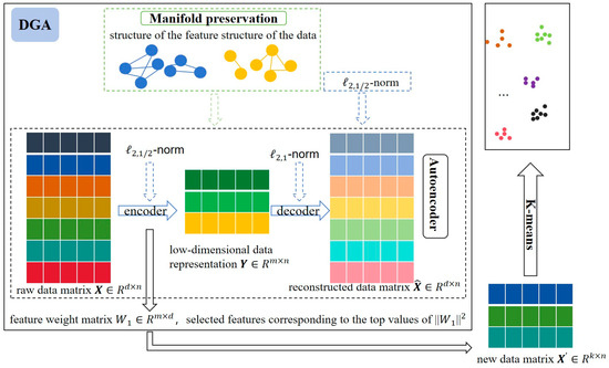
Figure 1. The structure of DGA (different colors represent different features).

(1) We embed dual-graph regularization into the autoencoder to preserve the manifold structures of both the data space and feature space during the reconstruction process.

(2) To promote sparsity and reduce feature redundancy, we impose ${\mathcal{l}}_{2,1/2}$-norm and ${\mathcal{l}}_{2,1}$-norm constraints on the weight matrices of the encoder and decoder, respectively, thereby enhancing the effectiveness of feature selection.

(3) To boost the robustness of the algorithm against noise and outliers present in real-world data, the ${\mathcal{l}}_{2,1/2}$-norm is introduced into the autoencoder’s loss function.

(4) We apply the proposed method to the publicly available [⁶⁸Ga]Ga-Pentixafor PET/CT images of glioma patients, performing unsupervised feature selection on PET scans. The results demonstrate the potential of our approach to assist in the diagnosis and analysis of gliomas by identifying discriminative features that characterize tumor regions.

The structure of the remainder of this paper is organized as follows. Section 2 reviews related work and presents the proposed method in detail, including the corresponding optimization strategies. Section 3 evaluates the performance of the proposed DGA by comparing it with several existing methods on nine benchmark datasets. Section 4 further demonstrates the effectiveness of the proposed method using the [⁶⁸Ga]Ga-Pentixafor PET/CT glioma dataset in an unsupervised clustering task. Finally, Section 5 concludes the paper with a summary of the key findings and potential directions for future research.

2. Related Work and Methods

2.1. Autoencoder

Neural networks have a strong ability to perform both linear and nonlinear mappings. They can learn arbitrary transformations and are well-suited for a wide range of tasks, including visual recognition and image segmentation. Among them, the autoencoder is a widely adopted neural network model known for its effectiveness in unsupervised feature learning and supervised dimensionality reduction tasks [21]. For intrusion detection, Zhang et al. [22] proposed SIGMOD, which integrates an improved Gaussian mixture model with a stacked sparse autoencoder. SIGMOD performs nonlinear dimensionality reduction through the autoencoder and determines sample anomalies based on reconstruction error. Manzoor and Halim Z [23] integrated three feature selection techniques to choose the optimal feature subset after unsupervised autoencoder feature extraction. Han et al. [19] leveraged autoencoders to represent each feature nonlinearly with varying weights and employed group sparse regularization to eliminate redundancy and achieve effective feature selection. Gong et al. [20] further improved the network structure by introducing Lasso regularization penalties, enhancing feature selection efficiency, and reducing computational complexity. Zhang et al. [24] explored the flexibility of autoencoder loss functions and activation functions to address various learning tasks. They innovatively applied orthogonal non-negative constraints, transforming the encoder’s weight matrix into an index matrix for feature selection. Li et al. [25] ntroduced the ACC_AN, which incorporates adaptive neighbor-based structured graph learning into deep autoencoder networks. This method preserves the data structure and enhances clustering performance.

In summary, the autoencoders exhibit exceptional capabilities in nonlinear mapping and model generalization. They can effectively generate high-quality data representations, reduce redundancy, and extract low-dimensional features. These characteristics make autoencoders highly suitable for unsupervised feature selection, ultimately enhancing the performance of downstream tasks such as clustering.

Autoencoders consist of a simple neural network whose goal is to transform input into output while preserving the same information as the input and minimizing distortion [22]. The primary constituents of an autoencoder comprise two components: an encoder and a decoder. For a single-layer autoencoder, the function $h\left(x,\theta \right)\approx x$ is learned through encoding and decoding. Considering a data matrix $X\in R^{d\times n}$, where d denotes the dimensions (i.e., the number of features) and n represents the sample size. The function $h\left(·\right)$ represents the nonlinear function, and $\theta$ represents the parameter set. More specifically, the workflow of an autoencoder consists of two steps:

Encoder. The encoder reduces the dimensionality of the raw data, compressing it into a low-dimensional space, thereby compelling the neural network to capture the most informative features present within it. Encoding process: mapping raw data X to a low-dimensional data representation $Y\in R^{m\times n}$.

$$Y=\sigma (W_{1}X+b_1)$$

(1)

In the equation, $W_1\in R^{m\times d}$ represents a weight matrix, $b_1\in R^m$ denotes a bias vector, and refers to the basic nonlinear activation function is represented by $\sigma (\cdot )$. The sigmoid function, hyperbolic tangent function, and rectilinear element are the most widely utilized activation functions.

Decoder. The low-dimensional representation of the hidden layer is restored to the original data dimension by the decoder, with the expectation that the output will fully or approximately recover the original input. Decoding process: transforming the low-dimensional data representation $Y$ back to the input space $\widehat{X}\in R^{d\times n}$.

$$\widehat{X}=\sigma (W_{2}Y+b_2)$$

(2)

where $W_2\in R^{d\times m}$ represents the weight matrix of the decoding layer and $b_2\in R^d$ denotes the corresponding bias vector.

The autoencoder expects as little difference as possible between the original data and the reconstructed output data. Specifically, for the dataset $X=[X^{(1)},X^{(2)},\cdots ,X^{(n)}]$, we perform network training to minimize the reconstruction error by continuously adjusting the parameters $W_1$, $W_2$, $b_1$, and $b_2$.

$${\displaystyle \sum _{i=1}^n\left|\right|X^{\left(i\right)}-{\widehat{X}}^{(i)}|{|}_2^2}$$

(3)

where ${\widehat{X}}^{(i)}$ represents the output of the autoencoder corresponding to input $X^{\left(i\right)}$. Typically, the backpropagation algorithm or alternative optimization techniques (such as gradient descent) are employed to optimize parameter values to reduce reconstruction errors [26]. Based on the backpropagation algorithm, the neural network attempts to learn a mapping relationship by utilizing the input data $X$ itself as supervision, thereby obtaining a reconstructed output $\widehat{X}$.

2.2. Dual-Graph Regularization

The presence of sparsity in high-dimensional data implies the abundance of structural information within. It is crucial to explore the concealed information. Typically, the Laplacian matrix is commonly utilized to maintain the local structural information inherent in the data. The main idea is that if two data points, $x_i$ and $x_j$, in the original space, are near to one another, then the two data points in the projected subspace should also demonstrate proximity. The following expression can be used to convey this idea:

$$\underset{x}{\min }{\displaystyle \frac{1}{2}}{\displaystyle \sum _i^n\left|\right|W^T{\mathit{x}}_i-W^T{\mathit{x}}_j|{|}_2^2{S}_{ij}=Tr(W^{T}X{L}^x{X}^{T}W)}$$

(4)

In this equation, $L^X$ is the Laplacian matrix of the data matrix $X$, while the similarity between sample $x_i$ and $x_j$ is denoted as $S_{\mathit{ij}}$. $L$ is obtained using the similarity matrix $S$ and the degree matrix $D$:

$$L=D-S$$

(5)

where $D$ is a diagonal matrix, defined as follows:

$$D=diag[{\displaystyle \sum _{j=1}^d(S_{1j}+S_{j1})}/2,{\displaystyle \sum _{j=1}^d(S_{2j}+S_{j2})}/2,,\dots ,{\displaystyle \sum _{j=1}^d(S_{nj}+S_{jn})}/2]$$

(6)

In this paper, the similarity is formulated by utilizing the Gaussian kernel function.

$$S_{ij}=\left\{\begin{array}{l}\exp (-||x_{.i}-x_{.j}|{|}_2^2),if x_{.i}\in \mathrm{\aleph }(x_{.j}) or x_{.j}\in \mathrm{\aleph }(x_{.i})\\ 0,else\end{array}\right.$$

(7)

For $X\in R^{d\times n}$, $\{x_{.1},x_{.2},\dots ,x_{.n}\}$ is a collection of n data points, with each being a column of $X$, and $\{x_{1.},x_{2.},\dots ,x_{d.}\}$ is the row of $X$, representing a set of d features. $\mathrm{\aleph }(x_{.i})$ represents the collection of the K nearest neighbors of x.

Nevertheless, the aforementioned methods primarily focus on preserving the manifold structure of the data space alone. Inspired by the duality between features (e.g., words) and data instances (e.g., documents)—where data instances can be characterized by their distributions over features, and features can be grouped based on their distributions across instances—researchers have proposed methods that capture more comprehensive structural information. For example, Gu and Zhou [16] introduced a Dual Regularized Co-Clustering (DRCC) technique based on semi-non-negative matrix tri-factorization, employing two graph structures to retain the geometric relationships of both data and feature manifolds. Their experimental results demonstrated improved clustering performance. Shang et al. [17] incorporated dual-graph regularization into non-negative matrix factorization (NMF), proposing the dual-graph regularization NMF (DNMF) algorithm to better exploit intrinsic structural information. Yin et al. [27] proposed a dual-graph regularized low-rank representation (DGLRR) model by integrating dual-graph constraints into a low-dimensional representation framework. Shang et al. [28] further developed a dual-graph regularization feature selection approach, combining non-negative spectral learning with sparse regression (NSSRD).

A growing body of work highlights that much real-world high-dimensional data—including its features—can be viewed as residing on nonlinear low-dimensional manifolds embedded in a high-dimensional space. Dual-graph regularization, which simultaneously preserves both the data and feature manifold structures, has shown great potential to enhance learning performance. However, its application remains largely confined to matrix factorization techniques and is seldom extended to other frameworks.

Equations (3) and (4) are the adjacency matrices of corresponding data and features. Then, $\mathrm{\aleph }(X_j)$ represents the collection of K neighbors.

$$S_{ij}^n=\left\{\begin{array}{l}\exp (-||x_{.i}-x_{.j}|{|}_2^2,if x_{.i}\in \mathrm{\aleph }(x_{.j}) or x_{.j}\in \mathrm{\aleph }(x_{.i})\\ 0,else\end{array}\right.$$

(8)

$$S_{ij}^d=\left\{\begin{array}{l}\exp (-||x_{i.}-x_{j.}|{|}_2^2,if x_{i.}\in \mathrm{\aleph }(x_{j.}) or x_{j.}\in \mathrm{\aleph }(x_{i.})\\ 0,else\end{array}\right.$$

(9)

Similarly, the issue of preserving local structure in the data and the feature space could be articulated as follows:

$$Tr(W^{T}X{L}^n{X}^{T}W) and Tr(W^{T}X{L}^d{X}^{T}W)$$

(10)

where $L^n=D^n-S^n$ and $L^d=D^d-S^d$.

2.3. Norm

For the matrix $A\in R^{d\times n}$, the $l_{q,p}$-norm is characterized as

$$\Vert A{\Vert }_{p,q}={\left({\displaystyle \sum _{j=1}^n({\displaystyle \sum _{i=1}^d|a_{ij}{|}^p{)}^{q/p}}}\right)}^{{\displaystyle \frac{1}{\mathrm{q}}}}$$

(11)

where $a_{ij}$ represents the $j$-th column vector in row $i$ of matrix $A$. Two commonly used norms are ${\mathcal{l}}_{2,1}$-norm and Frobenius norm (${\mathcal{l}}_{2,2}$).

In order to gain a deeper understanding of the role and principles of the ${\mathcal{l}}_{2,1}$-norm, Jiang and Ding [29] introduced a novel vector outlier regularization (VOR) function and then found that the outlier in ${‖X-UV‖}_{2,1}$ has much less impact on the final result than the square error. In other words, the ${\mathcal{l}}_{2,1}$-norm is insensitive to noise and anomalies. For multi-class classification, Nie et al. [2] used the ${\mathcal{l}}_{2,1}$-norm to increase sparsity. Zhu et al. [30] proposed co-regularization unsupervised feature selection (CUFS). CUFS applies the ${\mathcal{l}}_{2,1}$-norm to ensure sparsity in the projection matrix and cluster base matrix, which hold data reconstruction and cluster structure. Huang et al. [31] introduced the robust structured non-negative matrix factorization (RSNMF), which incorporates both the global and local structures of the data. This method tackles the challenges posed by noise and outliers by employing the ${\mathcal{l}}_{2,1}$-NMF optimization loss function. Furthermore, it enhances sparsity in the basis matrix through ${\mathcal{l}}_{2,1}$-regularization. The incorporation of ${\mathcal{l}}_{2,1}$-regularization improves the robustness of the algorithm suggested in this study.

A great multitude of computational studies have shown that sparser solutions can be obtained by using the ${\mathcal{l}}_{\mathrm{p}}$-norm (0 < p < 1) in contrast to using the ${\mathcal{l}}_1$-norm. Therefore, Wang et al. [32] further proved that the minimum solution based on generalized ${\mathcal{l}}_{2,\mathrm{p}}$-norm (p $\in$ (0,1)) has greater sparsity compared to that grounded in ${\mathcal{l}}_{2,1}$-norm and proposed a method to optimize the ${\mathcal{l}}_{2,\mathrm{p}}$-norm (p $\in$ (0,1)) that is non-convex and non-Lipschitz continuous, which proved its optimality and convergence. Since then, we have discovered the good performance of ${\mathcal{l}}_{2,\mathrm{p}}$-norm (p $\in$ (0,1)). Shi et al. [33] found that in the minimization process, ${\mathcal{l}}_{2,1/2}$ and ${\mathcal{l}}_{2,1-2}$ can obtain sparser solutions compared with ${\mathcal{l}}_{2,1}$ and ${\mathcal{l}}_{2,2}$. As shown in Figure 2, in the unsupervised feature selection proposed by Li and Tang [34] based on non-negative spectrum analysis and redundant control, ${\mathcal{l}}_{2,\mathrm{P}}$-norm constraints are imposed on the prediction matrix so that the proposed model is suitable for feature selection, and noisy or irrelevant features can be discarded to a certain extent. The semi-supervised NMF learning framework proposed by Li and Tang [34] learns robust discriminant representation using block diagonal structure and applying ${\mathcal{l}}_{2,\mathrm{P}}$-norm (especially when 0 < p ≤ 1) to the loss function. It is found that implementing the ${\mathcal{l}}_{2,\mathrm{P}}$-norm on the cost function can effectively address issues related to noise and outliers, especially when 0 < p < 1 and q = 2. Meng et al. [35] adopted the ${\mathcal{l}}_{2,1/2}$-norm regularization to induce sparsity of the matrix, thereby enhancing the stability of the algorithm and heightening the accuracy of clustering. For the same purpose, Lu et al. [26] used ${\mathcal{l}}_{2,1/2}$-norm for the cost function of non-negative matrix decomposition. Li et al. [36] used ${\mathcal{l}}_{2,1/2}$-norm to enhance matrix sparsity in the peer-to-peer projection matrix to make better feature selection.

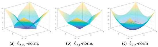
Figure 2. Contour plots of three different sparse matrices.

In summary, ${\mathcal{l}}_{2,\mathrm{P}}$-norm (p $\in$ (0,1)) can not only make the solution more sparse but also eliminate the impact of noise and outliers, so the robustness of the algorithm is enhanced. Different p values can be selected according to task requirements and characteristics, and ${\mathcal{l}}_{2,1/2}$-norm is commonly used at present.

2.4. Proposed Method

This section presents the unsupervised feature selection approach proposed in this study, which integrates an autoencoder with dual-graph regularization. The method embeds dual-graph regularization into a single-layer autoencoder to enable effective data reconstruction while preserving the geometric structures of both the data space and the feature space. This dual preservation guides the process of feature selection. In addition, by incorporating regularization constraints into both the loss function and the weight matrices, the proposed method achieves improved performance and enhanced robustness against noise and outliers.

2.4.1. Data Reconstruction Based on Autoencoder

According to Section 2.1, we reconstruct the data utilizing a single-layer autoencoder aiming to minimize the reconstruction error:

$$\min J(X;\widehat{X})=\min \Vert X-\widehat{X}{\Vert }_2^2=\min \Vert X-\sigma (Y+b_2){\Vert }_2^2$$

$$=\min \Vert X-\sigma (\sigma (W_1+b_1)+b_2){\Vert }_2^2$$

(12)

where the activation function used is the sigmoid function: $\sigma \left(z\right)=1/\left(1+exp\left(-z\right)\right)$.

In the coding process, $X$ is projected onto the latent space subspace, resulting in a low-dimensional representation of $Y$. In the coding layer, the weight matrix $W_1$ directly operates on the original data and serves as the projection matrix that maps the input data back into the subspace. Each column of the weight matrix $W_1$ quantifies the significance of its corresponding feature, thereby enabling feature selection to be performed using the weight matrix $W_1$. This is the main idea behind most current autoencoder-based feature selection approaches.

The loss function of existing autoencoders mostly adopts the sum of squares or F-norm, which is susceptible to outliers and noise. This sensitivity leads to high fluctuations in the results. It can be seen from Section 2.3 that the problem of noise and outliers can be solved by applying ${\mathcal{l}}_{2,1/2}$-norm to the loss function. Many people have applied it to the NMF, and we introduce it to autoencoders here.

At the same time, since autoencoder-based feature selection primarily measures the importance of features using the weight $W_1$ of the coding layer, enhancing the sparsity of the matrix is a critical method for selecting the most discriminative features. For instance, Han et al. [19] used ${\mathcal{l}}_{2,1}$ constraint on the weight matrix $W_1$. However, it is known that the solution obtained by ${\mathcal{l}}_{2,1/2}$-norm is sparser, so we apply ${\mathcal{l}}_{2,1/2}$-norm for $W_1$ to achieve a sparser solution. At the same time, Gong et al. [20] utilized ${\mathcal{l}}_{2,1}$ regularization constraints on the weight matrix to address issues such as poor generalization ability resulting from overfitting and excessive training time caused by an excessive number of hidden nodes in neural networks. In summary, the objective function is formulated as follows:

$$\min \Vert X-\widehat{X}{\Vert }_{2,1/2}^{1/2}+\lambda (\Vert W_1{\Vert }_{2,1/2}^{1/2}+\Vert W_2{\Vert }_{2,1})$$

(13)

where $\lambda$ represents a regularization parameter.

2.4.2. Local Structure Preservation Based on Dual-Graph Regularization

With the advancement of manifold learning, autoencoders have also employed various methods to maintain the data structure. However, the current methods primarily concentrate on the intrinsic structure of the data, disregarding the characteristic manifold. The dual-graph regularization considers both data manifolds and characteristic manifolds, preserving more comprehensive data information. Dual-graph regularization has been applied to NMF, but autoencoders reconstruct data using neural network backpropagation, which is a different method from NMF. We introduce it into autoencoders for the first time.

In combination with Section 2.2, in the autoencoder, for making the encoded low-dimensional representation, $Y$ retains the original information of the data as much as possible; the original data points $x_i$ and $x_j$ are adjacent, and the corresponding low-dimensional representation $y_i$ and $y_j$ are similarly close, that is, to minimize the target:

$$\underset{x}{\min }{\displaystyle \frac{1}{2}}{\displaystyle \sum _{i=1}^n{\displaystyle \sum _{j=1}^n{‖y_i-y_j‖}_2^2{s}_{ij}^n}}=\underset{x}{\min }Tr\left(Y{L}^n{Y}^T\right)=\underset{x}{\min }Tr\left(W^{T}X{L}^n{X}^{T}W\right)$$

(14)

Similarly, to keep the structure of the feature space, we expect $w_i$ and $w_j$ in the weight matrix $W_1$ that measures the significance of features. The association between the two is consistent with that between $x_i$ and $x_j$, that is, minimizing the goal:

$$\underset{x}{\min }{\displaystyle \frac{1}{2}}{\displaystyle \sum _{i=1}^d{\displaystyle \sum _{j=1}^d{‖w_i^{(1)}-w_j^{(2)}‖}_2^2}}{s}_{ij}^d=\underset{x}{\min }Tr\left(W_1{L}^d{W}_1^T\right)$$

(15)

In summary, the objective function of the unsupervised feature selection approach DGA presented in this research is as follows:

$$\underset{W_1,W_2}{\arg \min }{\displaystyle \frac{1}{n}}\Vert \widehat{X}-X{\Vert }_{2,{\displaystyle \frac{1}{2}}}^{{\displaystyle \frac{1}{2}}}+\lambda (\Vert W_1{\Vert }_{2,{\displaystyle \frac{1}{2}}}^{{\displaystyle \frac{1}{2}}}+\Vert W_2{\Vert }_{2,1})+\beta Tr(Y{L}^n{Y}^T)+\alpha Tr(W_1{L}^d{W}_1^T)$$

(16)

where $\lambda ,\alpha ,\beta (>0$) denote the parameter used to balance the regularization terms so that the model avoids overfitting and enhances robustness while retaining the inherent local geometry.

2.4.3. Optimization Method

${\mathcal{l}}_{2,1/2}$-norm possesses non-convex and non-Lipschitz continuous properties, and there is no universal method for solving such problems. In this paper, we still employ the commonly used gradient descent method in neural networks to calculate the optimization solution of the objective function.

The specific form of the objective function is as follows:

$$L(W_1;W_2;b_1;b_2)=J(X;\widehat{X})+\lambda (\Vert W_1{\Vert }_{2,{\displaystyle \frac{1}{2}}}^{{\displaystyle \frac{1}{2}}}+\Vert W_2{\Vert }_{2,1})+\beta \left(Tr(Y{L}^n{Y}^T)+(Tr(W_1{L}^d{W}_1^T)\right)$$

$$={\displaystyle \frac{1}{n}}\Vert \widehat{X}-X{\Vert }_{2,{\displaystyle \frac{1}{2}}}^{{\displaystyle \frac{1}{2}}}+\lambda (\Vert W_1{\Vert }_{2,{\displaystyle \frac{1}{2}}}^{{\displaystyle \frac{1}{2}}}+\Vert W_2{\Vert }_{2,1})+\beta Tr(Y{L}^n{Y}^T)+\alpha Tr(W_1{L}^d{W}_1^T)$$

(17)

The weight matrix $W_1$ is updated using gradient descent as follows:

$$W_1^{(t)}=W_1^{(t-1)}-\gamma \times {\nabla }_{{W_1}^{(\mathrm{t}-1)}}L(W_1;W_2;b_1;b_2)$$

(18)

where $W_1^{\left(t\right)}$ represents the t iteration of $W_1$, $\gamma$ represents the learning rate of the autoencoder, and ${\nabla }_{{W_1}^{(\mathrm{t}-1)}}L(W_1;W_2)$ represents the gradient of $W_1$. Furthermore, the gradient of $W_1$ is computed as follows:

$$\begin{array}{l}{\nabla }_{{W_1}^{(\mathrm{t}-1)}}L(W_1;W_2;b_1;b_2)={\displaystyle \frac{\partial L(W_1;W_2;b_1;b_2)}{\partial W_1}}\\ ={\displaystyle \frac{\partial J(W_1;W_2;b_1;b_2)}{\partial W_1}}+\lambda W_{1}D+\beta {\displaystyle \frac{\partial Tr(Y{L}^n{Y}^T)}{\partial W_1}}+\alpha {\displaystyle \frac{\partial Tr(W_1{L}^d{W}_1^T)}{\partial W_1}}\end{array}$$

(19)

where $D$ is a diagonal matrix:

$$D=diag\left\{{\displaystyle \frac{1}{2\times \left|\right|w_1^{(1)}|{|}_2^{\frac{3}{2}}}},{\displaystyle \frac{1}{2\times \left|\right|w_2^{(1)}|{|}_2^{\frac{3}{2}}}},\dots ,{\displaystyle \frac{1}{2\times \left|\right|w_m^{(1)}|{|}_2^{\frac{3}{2}}}}\right\}$$

(20)

where $w_m^{(1)}$ denotes the $m$-th row of $W_1$.

The derivative of the loss function $J\left(W_1;W_2;b_1;b_2\right)$ is as follows:

$${\displaystyle \frac{\partial J(W_1;W_2;b_1;b_2)}{\partial W_1}}={\displaystyle \frac{\partial \left|\right|\widehat{X}-X|{|}_{2,\frac{1}{2}}^{\frac{1}{2}}}{\partial W_1}}$$

$$={\displaystyle \frac{1}{n}}(W_2^T({\displaystyle \frac{\widehat{X}-X}{2\left|\right|\widehat{X}-X|{|}_2^{3/2}}}\cdot \widehat{X}\cdot [1-\widehat{X}]))\cdot Y\cdot [1-Y]X^T$$

(21)

where the element-wise product operator is indicated by $\cdot$, the activation function σ is the sigmoid function $Y=\left(W_1+b_1\right)$.

$${\displaystyle \frac{\partial Tr(Y{L}^n{Y}^T)}{\partial W_1}}=2Y{L}^n\cdot Y\cdot (1-Y)X^T$$

$${\displaystyle \frac{\partial Tr(W_1{L}^d{W_1}^T)}{\partial W_1}}=2W_1{L}^d$$

(22)

In a similar vein, iterative calculation yields the weight matrix $W_2$:

$$W_2^{(t)}=W_2^{(t-1)}-\gamma \times {\nabla }_{{W_2}^{(\mathrm{t}-1)}}L(W_1;W_2;)=W_2^{(t-1)}-\gamma \times {\displaystyle \frac{\partial L(W_1;W_2;b_1;b_2)}{\partial W_2}}$$

(23)

$${\displaystyle \frac{\partial L(W_1;W_2;b_1;b_2)}{\partial W_2}}={\displaystyle \frac{\partial J(W_1;W_2;b_1;b_2)}{\partial W_2}}+\lambda B{W}_2$$

(24)

$$B=diag\left\{{\displaystyle \frac{1}{\left|\right|w_1^{(2)}|{|}_2}},{\displaystyle \frac{1}{\left|\right|w_2^{(2)}|{|}_2}},\dots ,{\displaystyle \frac{1}{\left|\right|w_d^{(2)}|{|}_2}}\right\}$$

(25)

where $w_d^{(1)}$ denotes the $d$-th row of $W_2$.

In a similar way, $b_1$ and $b_2$ terations are calculated as follows:

$$b_1^{(t)}=b_1^{(t-1)}-\gamma \times {\nabla }_{{b_1}^{(t-1)}}L(W_1;W_2;b_1;b_2)=b_1^{(t-1)}-\gamma \times {\displaystyle \frac{\partial L(W_1;W_2;b_1;b_2)}{\partial b_1}}$$

(26)

$$b_2^{(t)}=b_2^{(t-1)}-\gamma \times {\nabla }_{{b_2}^{(\mathrm{t}-1)}}L(W_1;W_2;b_1;b_2)=b_2^{(t-1)}-\gamma \times {\displaystyle \frac{\partial L(W_1;W_2;b_1;b_2)}{\partial b_2}}$$

(27)

According to the updating rules for DGA presented above, the overall optimization process is given in Algorithm 1.

Algorithm 1. Unsupervised feature selection method based on dual-graph autoencoder (DGA)
Input:	Data matrix $X\in R^{m\times n}$ hidden layer size: $m$ KNN parameter $k$ learning rate $\gamma$ balance parameters $\beta ,\lambda ,\alpha$
Output:	The selected subset of the features.
1:	Initialize the parameters ${\mathit{W}}_1\in R^{m\times d}$, ${\mathit{W}}_2\in R^{d\times m}$, $b_1\in R^m$, $b_2\in R^d$ of auto-encoders;
2:	repeat
3:	Calculate loss of auto-encoder by Equation (17);
4:	Update ${\mathit{W}}_1$ by Equation (18);
5:	Update the $j$-th diagonal element of D by ${\displaystyle \frac{1}{2\times \left|\right|w_j^{(1)}|{|}_2^{3/2}}}$;
6:	Update ${\mathit{W}}_2$ by Equation (23)
7:	Update the jth diagonal element of B by ${\displaystyle \frac{1}{2\times \left|\right|w_j^{(2)}|{|}_2}}$;
8:	Update ${\mathit{b}}_1$ by Equation (26);
9:	Update ${\mathit{b}}_2$ by Equation (27);
10:	until Convergence
	Return Selected features corresponding to the top k values of ||W1||2, which are sorted by descending order

2.4.4. Computational Complexity Analysis

In this section, the computational complexity of the algorithm that this study proposes is analyzed.

To construct the KNN graph in a dataset $X\in R^{d\times n}$, the time complexity is typically calculated as $\mathcal{O}\left(d{n}^2\right)$, where $n$ and $d$ are the number of samples and features of the data, respectively. For our method, we calculate similarity based on both data and features. The time complexity of constructing a KNN graph for the entire dataset is $\mathcal{O}\left(d{n}^2+n{d}^2\right)$.

The optimization objective function (17) has a temporal complexity of $\mathcal{O}\left(d{m}^2+m{d}^2\right)$, where $m$ represents the size of the hidden layer. By the gradient descent approach, the cost of each iteration for updating $W_1$, $W_2$, $b_1$, and $b_2$ is $\mathcal{O}\left(m{d}^2\right)$, $\mathcal{O}\left(m{d}^2\right)$, $\mathcal{O}\left(dn+mnd+mn\right)$ and $\mathcal{O}\left(md\right)$, respectively. The entire computational complexity after t iterations is $\mathcal{O}\left(td{m}^2+tm{d}^2\right)$.

After obtaining $W_1$, we need $\mathcal{O}\left(dn\right)$ to compute the score for each feature. Then, we sort the results, which takes a very short period.

Therefore, the overall time complexity of DGA is $\mathcal{O}\left(d{n}^2+n{d}^2+tm{d}^2+t{m}^{2}d\right)$.

3. Results

In this section, we conduct comprehensive experiments on nine publicly available datasets to evaluate the effectiveness of the proposed DGA method in comparison with five state-of-the-art approaches. Prior to presenting the results, we provide a detailed explanation of the parameter settings and evaluation metrics used in the experiments. The experimental outcomes are subsequently analyzed to demonstrate the performance, robustness, and advantages of our method. All experiments were implemented using Python 3.8 and executed on a Windows 10 system running on a server equipped with an Intel Core i5-8250U CPU and 12.0 GB of RAM.

3.1. The Experimental Preparation

3.1.1. Datasets

In this study, comprehensive experiments are conducted on nine publicly available benchmark datasets to evaluate the effectiveness of the proposed feature selection method. Prior to the experiments, detailed descriptions of the parameter settings and evaluation metrics are provided. For the benchmark datasets—which include diverse data types such as facial images, object images, and gene expression data—200 samples were randomly selected from each digit class in the MNIST dataset [26]. MNIST is a large-scale dataset of handwritten digits widely used for image classification and machine learning benchmarking. It contains 70,000 grayscale images of size 28 × 28 pixels, divided into 60,000 training and 10,000 testing samples, covering digits from 0 to 9. All datasets used in this study are publicly available benchmark datasets, which can be accessed through the scikit-feature selection library [6]. Table 1 summarizes the detailed specifications of all datasets used.

Table 1. Details of the datasets.

ID	Datasets	Instances	Features	Classes	Data Types	Description
1	Isolet [6]	1560	617	26	Image, text	UCI dataset
2	Mnist [26]	2000	784	10	Image, text	Handwritten digits, 28 × 28 pixels
3	Yale (32*32) [6]	165	1024	15	Image, Face	Yale face database, 32*32 grayscale
4	ORL (32*32) [6]	400	1024	40	Image, Face	AT&T face dataset
5	COIL20 [6]	1440	1024	20	Image, Object	Columbia object images
6	WarpAR10P [6]	130	2400	10	Image, Face	Cropped face images under different conditions
7	WarpPIE10P [6]	210	2420	10	Image, Face	PIE face dataset, cropped
8	Colon [6]	62	2000	2	Gene expression, Biology	Tumor vs. normal colon tissue
9	TOX-171 [6]	171	5748	4	Gene expression, Biology	Toxicogenomic gene expression data

3.1.2. Evaluation Metrics

The performance of feature selection algorithms in clustering is evaluated by using two generally used measurements: clustering accuracy (ACC) and normalized mutual information (NMI) [37]. Then, the metric ACC is denoted as follows:

$$ACC={\displaystyle \frac{1}{n}}{\displaystyle \sum _{i=1}^n\delta (p_i,map(q_i))}$$

(28)

The cluster label and the actual label of the sample $x_i$ are represented by $p_i$ and $q_i$, respectively. If $x=y$, $\delta \left(x,y\right)=1$, otherwise $\delta \left(x,y\right)=0$. $map\left(\cdot \right)$ utilizes the Kuhn–Munkres algorithm to establish a one-to-one correspondence between cluster labels and their corresponding true labels is an optimal permutation mapping function [2]. ACC ranges from 0 to 1, and the higher the value, the greater the performance.

The NMI is defined as follows:

$$NMI={\displaystyle \frac{I(P,C)}{\sqrt{H(P)H(C)}}}$$

(29)

Two arbitrary variables are given, P and C, where the mutual information between $P$ and $C$ is represented by $I(P,C)$. Then the entropy of $P$ and $C$ are represented as $H\left(P\right)$ and $H\left(C\right)$, respectively. During this experiment, $P$ and $C$ represent the clusters and true labels of the sample. It should be noted that the closer ACC and NMI are to one, the greater the clustering performance.

To further verify whether the performance is superior compared to other algorithms, model performance evaluation methods are required: the Friedman test and the Nemenyi post hoc test. These two methods are particularly useful for comparing multiple algorithms.

First, calculate the rank values corresponding to each model. The algorithms are ranked based on their test performance on each dataset (in this study, using ACC and NMI). If the test performance of the algorithms is identical, the ranks are averaged. Let there be N datasets and K models. Denote the rank of the $i$-th model on the $j$-th data set as $ran{k}_{i,j}$. Then, the rank of the $i$-th model is

$$r_i={\displaystyle \frac{1}{N}}{\displaystyle \sum _{j=1}^{N}ran{k}_{i,j}}$$

(30)

Then, calculate the corresponding statistical quantities. Assuming that the rank of each model follows a normal distribution, the corresponding chi-square statistic is given by

$${\tau }_{{\chi }^2}={\displaystyle \frac{k-1}{k}}{\displaystyle \frac{12N}{k^2-1}}{\displaystyle \sum _{i=1}^k(r_i}-{\displaystyle \frac{k+1}{2}}{)}^2={\displaystyle \frac{12N}{k(k+1)}}({\displaystyle \sum _{i=1}^k(r_i^2}-{\displaystyle \frac{k{(k+1)}^2}{4}})$$

(31)

When both $k$ and $N$ are relatively large, the chi-square statistic follows a chi-square distribution with $k-1$ degrees of freedom. The improved statistic is

$${\tau }_F={\displaystyle \frac{(N-1){\tau }_{\chi }^2}{N(k-1)-{\tau }_{\chi }^2}}$$

(32)

The test statistic ${\tau }_F$ follows an F-distribution with degrees of freedom $k-1$ and $\left(k-1\right)\left(N-1\right)$. The critical values can be obtained from standard F-distribution tables. If the null hypothesis is rejected, it indicates a significant difference in the performance of the algorithms, and a post hoc test is then employed to further distinguish between the algorithms. A commonly used post hoc test is the Nemenyi test. The Nemenyi test calculates the critical value range for the difference in average ranks between the algorithms:

$$CD=q_{\alpha }\sqrt{{\displaystyle \frac{k(k+1)}{6N}}}$$

(33)

The $q_{\alpha }$ for different confidence levels can be obtained from the table. If the difference in the mean ranks of two algorithms exceeds the critical value range (CD), the hypothesis that “the two algorithms have the same performance” is rejected with the corresponding confidence level.

3.1.3. Algorithms Compared

The suggested approach aims to acquire the geometric characteristics of the data and select features using an autoencoder-based approach. For the purpose of assessing the efficacy of DGA, the suggested algorithms are compared with a set of seven representative algorithms:

• Baseline: Select all features;
• LS ([2]): The Laplacian Score approach, which chooses the features with the greatest variance while effectively preserving the local manifold structure of the data;
• SCFS ([12]): Unsupervised feature selection for subspace clustering, using self-expression models to learn cluster similarity to select discriminant features;
• UDFS ([38]): Uses the discriminant information of local structure and l_2,1-norm regularization discriminant to select features;
• MCFS ([13]): Clustering feature selection grounded in spectral analysis and sparse regularization;
• DUFS ([39]): Applies the dependency information among features to the unsupervised feature selection process based on regression;
• NLRL-LE ([10]): A feature selection method via non-convex constraint and latent representation learning with Laplacian embedding;
• LLSRFS ([40]): A unified framework for optimal feature combination combining local structure learning and exponentially weighted sparse regression.

3.1.4. Parameter Selection

The parameters of the comparison method are selected according to the optimization method of the corresponding paper. The k-nearest neighbor algorithm adjusts the parameter $k$ from $\left\{3,5,7,9,11,13,15\right\}$ for LS, UDFS, and MCFS. For LS, the bandwidth parameter σ of the Gaussian kernel is set to a constant value of 10. For SCFS, as stated in the original article by Parsa et al., the parameter $\gamma$ is held constant at 106, and the values of the other parameters are adjusted from $\left\{{10}^{-4},{10}^{-2},{10}^0,{10}^2,{10}^4\right\}$. Other weight parameters in DUFS and UDFS are searched from $\left\{{10}^{-6},{10}^{-5},{10}^{-4},\dots ,{10}^4,{10}^5,{10}^6\right\}$.

For the proposed algorithm DGA, it is necessary to preset six parameters. These parameters include the graph nearest neighbor k, the weight regularization parameter λ, the dual-graph regularization parameter $\beta$ and $\alpha$, the auto-encoder hidden layer m, and the learning rate $\gamma$. Similar to other algorithms, the value of the neighbor number k is adjusted starting from $\left\{3,5,7,9,11,13,15\right\}$. Then, the parameters $\lambda$, $\beta$, and $\alpha$ are optimized from $\left\{{10}^{-6},{10}^{-5},{10}^{-4},\dots ,{10}^4,{10}^5,{10}^6\right\}$, while $\gamma$ is optimized from $\left\{{10}^{-6},5\times {10}^{-5},{10}^{-5},5\times {10}^{-4},{10}^{-4},\dots ,{10}^4,5\times {10}^4,{10}^5,5\times {10}^5,{10}^6\right\}$. Additionally, the parameter m is selected from the set $\left\{5, 50, 100, 150,200,250,300\right\}$.

We employ the k-means clustering algorithm to assess the performance of each approach mentioned above, where the value of k is the number of classes in each dataset. For each dataset, the selected features range from 10 to 300, with an interval of 10. Firstly, the feature set is acquired through the utilization of diverse feature selection algorithms. Subsequently, the obtained feature set is subjected to clustering using the k-means algorithm. Analyze the clustering results of each approach and the best clustering outcome is reported.

3.2. Classification Results

The ACC and NMI clustering results of nine datasets using the K-means algorithm are presented in Table 2. Bold values represent the best result under this dataset, while underscores indicate suboptimal outcomes. As evident from Table 2, it can be observed that DGA exhibits promising performance.

Table 2. The best accuracy (ACC) and normalized mutual information (NMI) of various feature selection algorithms. (The best and second-best outcomes are indicated by bold and underlined text, respectively).

		All Features	LS	SCFS	UDFS	MCFS	DUFS	DGA
ACC	Isolet	0.658	0.612	0.721	0.528	0.578	0.602	0.755
	mnist	0.519	0.469	0.5895	0.507	0.566	0.5575	0.6235
	Yale (32*32)	0.418	0.4667	0.442	0.442	0.406	0.419	0.527
	ORL (32*32)	0.5675	0.555	0.63	0.5275	0.62	0.58	0.645
	COIL20	0.6889	0.617	0.731	0.637	0.707	0.686	0.739
	WarpAR10P	0.238	0.384	0.353	0.3	0.323	0.292	0.392
	WarpPIE10P	0.2621	0.385	0.323	0.342	0.371	0.48	0.433
	colon	0.532	0.564	0.645	0.548	0.564	0.548	0.612
	TOX-171	0.415	0.438	0.479	0.431	0.426	0.549	0.485
NMI	Isolet	0.791	0.745	0.816	0.669	0.721	0.752	0.818
	mnist	0.458	0.361	0.513	0.441	0.453	0.5055	0.498
	Yale (32*32)	0.487	0.52	0.495	0.488	0.459	0.425	0.55
	ORL (32*32)	0.76	0.744	0.781	0.721	0.793	0.759	0.804
	COIL20	0.791	0.744	0.792	0.747	0.782	0.751	0.803
	WarpAR10P	0.21718	0.438	0.304	0.254	0.338	0.278	0.38
	WarpPIE10P	0.236	0.39	0.323	0.288	0.372	0.536	0.425
	colon	0.045797	0.06425	0.03363	0.03122	0.08478	0.03122	0.154
	TOX-171	0.127	0.169	0.228	0.173	0.141	0.301	0.267

Table 2 presents the results compared with several classic algorithms. Additionally, we compare with two newer algorithms. Following the same procedures as NLRL-LE ([10]) and LLSRFS ([40]), we repeated the k-means clustering 20 times and averaged the results to obtain the final clustering outcome. The results are shown in Table 3. It can be observed that, except for the WarpPIE10P and TOX-171 datasets, DGA outperforms the other two methods in terms of ACC across the remaining datasets. While DGA’s overall NMI performance is not particularly outstanding, the differences in NMI values compared to the other two methods are minor. Overall, DGA exhibits a strong performance compared to the latest algorithms.

Table 3. Comparison of accuracy (ACC) and normalized mutual information (NMI) between the two novel methods across all datasets presented as mean ± standard deviation. (The best outcomes are indicated by bold).

	ACC			NMI
	NLRL-LE	LLSRFS	DGA	NLRL-LE	LLSRFS	DGA
Isolet	0.7071 ± 0.0201	0.6517 ± 0.0067	0.7472 ± 0.0114	0.7869 ± 0.0104	0.7848 ± 0.0052	0.812 ± 0.004
mnist	0.5765 ± 0.0142	-	0.6172 ± 0.0042	0.4986 ± 0.006	-	0.5004 ± 0.0039
Yale (32*32)	-	0.4856 ± 0.0040	0.5054 ± 0.0124	-	0.5652 ± 0.0062	0.5442 ± 0.0061
ORL (32*32)	-	0.6113 ± 0.0073	0.632 ± 0.0154	-	0.7930 ± 0.0056	0.7920 ± 0.0071
COIL20	0.6797 ± 0.0406	0.7357 ± 0.0053	0.743 ± 0.021	0.7742 ± 0.0180	0.8335 ± 0.0024	0.8085 ± 0.0036
WarpAR10P	-	-	0.3785 ± 0.0049	-	-	0.3645 ± 0.0190
WarpPIE10P	0.5357 ± 0.0256	-	0.4238 ± 0.0158	0.5666 ± 0.0235	-	0.3994 ± 0.0173
colon	-	-	0.608 ± 0.004	-	-	0.100 ± 0.029
TOX-171	0.5465 ± 0.0150	0.5268 ± 0.0174	0.468 ± 0.062	0.2295 ± 0.0157	0.3574 ± 0.0076	0.206 ± 0.027

Furthermore, we employed the Friedman test followed by the Nemenyi post hoc test to validate the performance of the proposed models, with the results presented in Table 4. At α = 0.1, the Friedman test statistics for ACC and NMI metrics exceeded the critical value of 1.9006. Indicating significant differences in the performance among the compared algorithms. The Nemenyi post hoc test further discriminates these algorithmic differences. According to the Critical Difference (CD) diagram (Figure 3), we observe that apart from SCFS, DGA shows minimal overlap with other algorithms in terms of ACC and NMI. The pairwise rank differences with SCFS are 1.388 and 1.7778 for ACC and NMI, respectively, which are below the critical value of 2.742. Therefore, it is evident that DGA exhibits significantly different performance compared to the other algorithms, except for SCFS.

Table 4. Friedman and Nemenyi post hoc test ($\mathsf{\alpha }$ = 0.1, number of algorithms = 7, number of datasets = 9).

	$\mathbf{Friedman} \mathbf{Test} ({\mathit{\tau }}_{\mathit{F}}$) (1.9006)	Nemenyi Post Hoc Test (CD)
ACC	${\tau }_F$ = 8.192771084337322	CD = 2.742416965892462
NMI	${\tau }_F$ = 5.23896388179497	CD = 2.742416965892462

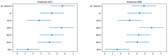
Figure 3. Nemenyi post hoc test (Critical Difference diagram).

Among these datasets, optimal results are observed in six cases, whereas the remaining three datasets exhibit sub-optimal outcomes. Notably, when applied to Yale, the clustering accuracy of this algorithm improves by 12.9% in comparison to the second algorithm. For mnist and Isolet datasets, when compared to the second-ranked algorithm, this algorithm has demonstrated an increase in clustering accuracy by 5.76% and 4.71%, respectively. In addition, the findings indicate that the DGA outperforms the baseline approach across all nine datasets, thereby affirming the indispensability of feature selection. The NMI results for the mnist dataset, while not exceptional, are moderate and surpass the baseline. This indicates that feature selection enhances its performance. Among the datasets analyzed, the performance of the SCFS algorithm was found to be comparable to that of the DGA in nine datasets. However, it was observed that the results obtained from SCFS were slightly inferior to those obtained from DGA. The reasons can be outlined as follows: (1) both approaches take into account the preservation of data structures, and (2) SCFS solely focuses on the manifold structure of the data; it disregards the manifold structure of the features.

The ACC and NMI of the clustering outcomes when varying numbers of features are selected are presented in Figure 4 and Figure 5, respectively. In accordance with Figure 4, it is evident that no matter how many features are selected, the performance of the DGA on datasets such as ORL (32*32), Isolet, Coll20, colon, Yale (32*32), and mnist is consistently superior to that of other algorithms. On the remaining three datasets, the performance of DGA was slightly inferior compared to the other methods. Similarly, Figure 5 demonstrates that. In the majority of cases, the DGA algorithm outperforms other algorithms on datasets such as ORL (32*32), Isolet, Coll20, colon, and Yale (32*32). On the remaining four datasets, the DGA also achieved the second-best performance, falling slightly short of the optimal solution. Therefore, it can be inferred that DGA possesses certain advantages in comparison to alternative methods.

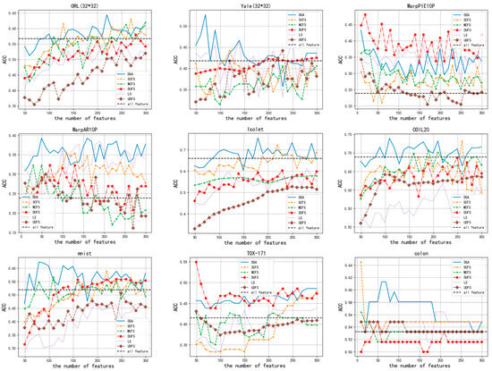
Figure 4. The ACC scores for clustering outcomes with different numbers of selected features.

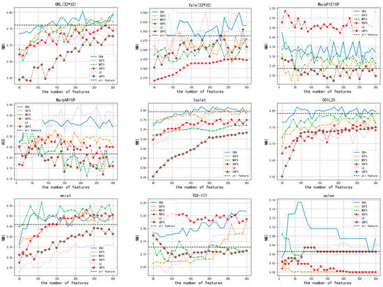
Figure 5. The NMI scores for clustering outcomes with different numbers of selected features.

Additionally, we present the visual representation of every comparison technique on the PET dataset with 100 features chosen in Figure 6. It is evident that the feature set selected by UDFS primarily focuses on the left part of the image, while the features selected by LS are scattered.

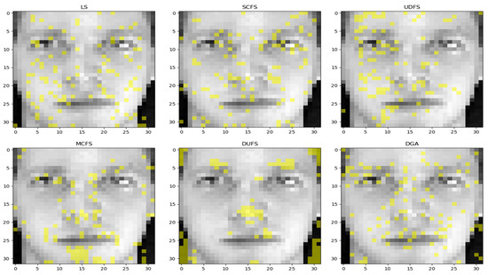
Figure 6. Visualizations of the suggested method and all compared algorithms on the ORL dataset, with k = 100 features selected for each method.

For DUFS, it selected a few salient features, such as the eyes and nose, as well as outlines, and most of the selection results for the eye area were located on top. For MCFS visualization, the key features are almost all selected. Both SCFS and our proposed method, DGA, effectively select all the key features, and the distribution of these features in the selected areas is relatively uniform. The high accuracy achieved by these two methods serves as a strong indication that the majority of the important features have been successfully identified

3.3. Convergence Analysis

The convergence of DGA is represented through line graphs. The convergence curve, obtained by testing on all nine datasets, documents the variation in the objective function throughout different iterations. All parameters were held constant throughout the experiment. As depicted in Figure 7, the value of the objective function gradually converges with an increasing number of iterations.

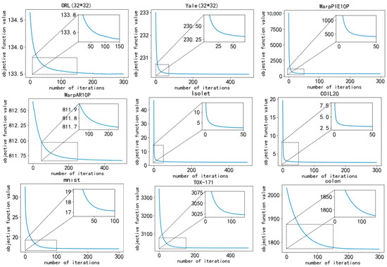
Figure 7. Convergence curves of the objective function value.

3.4. Parameter Sensitivity Analysis

Regarding DGA, six parameters are subject to investigation, namely, $\lambda$, $\alpha$, $\beta$, $k$, $m$, and $\gamma$. Based on our experiments and the experience of others, it has been observed that setting the nearest neighbor parameter $k$ to either 3 or 5 yields superior results. In this study, we set the value of k to 5. As for the learning rate $\gamma$, we make adjustments based on the observed convergence effect of the loss function. The remaining parameters are obtained by searching from $\left\{{10}^{-3}, {10}^{-2}, {10}^{-1}, 1, {10}^1, {10}^2, {10}^3\right\}$. The performance of the ACC performance on six datasets, namely COIL20, Isolet, ORL, WarpAR10P, warpPIE10P, and colon, is reported in Figure 8, Figure 9, Figure 10 and Figure 11, taking into account the limited space available.

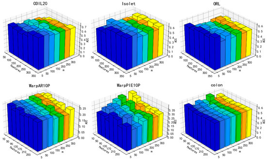
Figure 8. Parameter sensitivity in relation to ACC for the parameter m ($\mathsf{\lambda }=0.01,\mathsf{\alpha }=1,\mathsf{\beta }=1$).

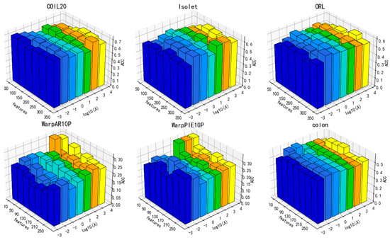
Figure 9. Parameter sensitivity in relation to ACC for the parameter $\mathsf{\lambda }$ ($\mathsf{\beta }=1,\mathsf{\alpha }=$1, m = 5).

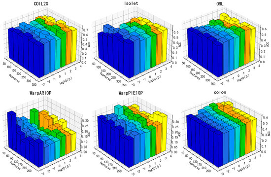
Figure 10. Parameter sensitivity in relation to ACC for the parameter $\mathsf{\beta }$ ($\mathsf{\lambda }=0.01,\mathsf{\alpha }=1$, m = 5).

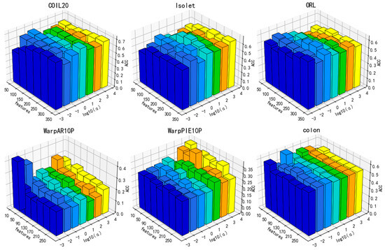
Figure 11. Parameter sensitivity in relation to ACC for the parameter $\mathsf{\alpha }$ ($\mathsf{\lambda }=0.01,\mathsf{\beta }=1,\mathrm{m}=5$).

In Figure 8, it can be observed that as the hidden layer m changes, the clustering accuracy fluctuates to some extent. But, in general, as the variable m increases, there is a decrease in the value of ACC. A smaller m means that the lower the dimensionality space of the mapping, the more sufficient the measurement of the significance of each feature. Hence. In the subsequent experiments, m will be held constant at 5.

Additionally, the performance of DGA varies under the influence of parameters, as illustrated in Figure 9, Figure 10 and Figure 11. As can be deduced from the figure, the experimental performance of the model is significantly influenced by these three parameters, and the sensitivity of the parameters varies across different datasets.

The parameters β and α exhibit greater fluctuations across each dataset. Overall, the clustering accuracy initially increases and then subsequently decreases as the values of these two parameters increase. A lower number indicates inadequate preservation of data and feature structures, whereas a higher value may overfit the manifold structure of the data. Overall, there is a decrease in the number of features that correspond to the optimal value of clustering accuracy with the increase in parameter values. Increasing the parameters β and α means that more of the manifold structure of the data and features are preserved. This allows for the selection of fewer features that can contain more complete information.

As a result, parameter selection is critical for our approach.

4. Application

4.1. Dataset

In this study, comprehensive experiments are conducted on the [⁶⁸Ga]Ga-Pentixafor PET/CT images of glioma patients [41], which includes data from 24 treatment-naïve adult patients diagnosed with high-grade glioma. Each patient received an intravenous injection of a radiolabeled CXCR4-targeting tracer, followed by PET/CT imaging approximately 60 min post-injection. Scanning was performed with a dedicated PET/CT system, acquiring images at 10 min per bed position. The data were reconstructed using a 3D-OSEM algorithm incorporating point spread function (PSF) resolution recovery (TrueX, Syngo^® software (VB80A), Siemens Medical Solutions), with 3 iterations, 21 subsets, and a 3 mm Gaussian post-smoothing filter. For analysis, the middle 128 slices were selected from each patient’s scan, each representing a region of interest (ROI) within the glioma tumor. For the glioma dataset, the selected features are evaluated using K-means clustering to assess their ability to distinguish between different tumor regions, such as active tumor tissue and necrotic areas. The experimental results demonstrate that the selected features contribute to effective clustering and hold potential value for tumor characterization.

4.2. Clustering Evaluation Metrics

To quantitatively evaluate the quality of the selected feature subsets, we adopted three widely used internal clustering validation indices that measure the compactness, separation, and balance of clusters without requiring ground truth labels:

• Silhouette Coefficient (SC): The Silhouette Coefficient quantifies how well each sample lies within its cluster compared to other clusters. For a sample $i$, it is defined as

  $$s\left(i\right)={\displaystyle \frac{b\left(i\right)-a\left(i\right)}{\max \left\{a\left(i\right),b\left(i\right)\right\}}}$$

  (34)

  where $a\left(i\right)$ is the average intra-cluster distance (compactness) and $b\left(i\right)$ is the smallest average inter-cluster distance (separation) between sample $i$ and all samples in other clusters. The goal SC is the mean of $s\left(i\right)$ overall samples, ranging from −1 (worst) to 1 (best);
• Davies-Bouldin Index (DBI): The Davies–Bouldin Index evaluates the average similarity between each cluster and its most similar counterpart. It is defined as follows:

  $$DBI={\displaystyle \frac{1}{k}}{\displaystyle \sum _{i=1}^k\underset{j\ne i}{\max }}\left({\displaystyle \frac{{\sigma }_i+{\sigma }_j}{d\left(c_i,c_j\right)}}\right)$$

  (35)

  where ${\sigma }_i$ is the average distance from samples in cluster $i$ to its centroid $c_i$, and $d\left(c_i,c_j\right)$ is the distance between centroids $c_i$ and $c_j$. Lower DBI values indicate better clustering performance.
• Calinski–Harabasz Index (CHI): The Calinski–Harabasz Index measures the ratio of between-cluster dispersion to within-cluster dispersion:

  $$CHI={\displaystyle \frac{Tr\left(B_k\right)}{Tr\left(W_k\right)}}\times {\displaystyle \frac{N-k}{k-1}}$$

  (36)

  where $B_k$ and $W_k$ are the between-cluster and within-cluster covariance matrices, $k$ is the number of clusters, and N is the total number of samples. A higher CHI value indicates better-defined clusters.

These metrics collectively assess the trade-off between intra-cluster cohesion and inter-cluster separation, providing a comprehensive evaluation of feature subsets in unsupervised scenarios.

4.3. Comparing Results

First, to evaluate the effectiveness of the proposed feature selection method in tumor region segmentation, especially in distinguishing active tumor regions from necrotic regions, we used K-means cluster analysis. This unsupervised learning method allows us to thoroughly assess the role of features in tumor region segmentation by clustering feature data points into distinct clusters. Through K-means cluster analysis, we divided the tumor region into two clusters: the active tumor region and the necrotic region. Figure 12 presents the visualization results of our method alongside other feature selection techniques. As shown in the figure, the proposed method demonstrates superior accuracy in delineating tumor boundaries and extracting overall image features. Clinically, accurate segmentation of tumor regions—especially in distinguishing active tumor areas from necrotic ones—can significantly aid in treatment planning, such as radiation therapy or surgery, by providing better-targeted intervention. This ability to refine tumor characterization can also help monitor the progression or regression of the tumor, allowing for more informed decision-making regarding patient care.

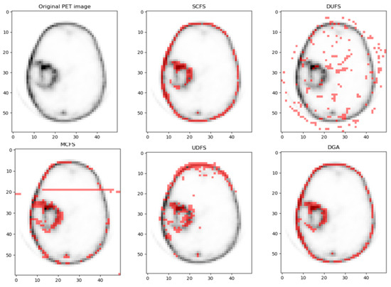
Figure 12. Visualizations of the suggested method and all compared algorithms on the PET dataset, with k = 200 features selected for each method.

Next, to validate the effectiveness of the proposed feature selection method in preserving intrinsic data structures, we compared the clustering quality of different methods using three internal validation indices: Silhouette Coefficient (SC), Calinski–Harabasz Index (CHI), and Davies–Bouldin Index (DBI). As shown in Table 5, the proposed method achieved the highest SC (0.41 ± 0.02) and CHI (275.8 ± 22.5), along with the lowest DBI (1.12 ± 0.07), outperforming all baseline and state-of-the-art methods.

Table 5. Internal clustering validation of feature selection methods on [⁶⁸Ga]Ga-Pentixafor PET/CT glioma data. (The best outcomes are indicated by bold).

Method	SC	CHI	DBI
Baseline	0.21 ± 0.03	152.3 ± 12.1	1.98 ± 0.15
SCFS	0.28 ± 0.04	198.6 ± 15.7	1.67 ± 0.13
UDFS	0.30 ± 0.03	223.1 ± 16.9	1.53 ± 0.09
MCFS	0.35 ± 0.02	268.4 ± 20.3	1.38 ± 0.08
DUFS	0.31 ± 0.03	234.5 ± 17.6	1.49 ± 0.10
DGA	0.41 ± 0.02	275.8 ± 22.5	1.12 ± 0.07

The proposed method significantly improved cluster compactness and separation compared to the baseline (0.41 vs. 0.21, p < 0.001, t-test), indicating that the selected features better distinguish glioma subtypes. Notably, it surpassed SCFS by 46.4%, suggesting enhanced robustness to noise in PET/CT imaging. For CHI, the higher CHI value (275.8 vs. 268.4 for MCFS) demonstrates a more favorable balance between intra-cluster homogeneity and inter-cluster heterogeneity. This aligns with the biological diversity of glioma phenotypes (e.g., IDH-mutant vs. wild-type) captured by [⁶⁸Ga]Ga-Pentixafor PET features. For DBI, the lower DBI (1.12 vs. 1.38 for MCFS) implies reduced overlap between clusters, which is critical for precise patient stratification in clinical practice.

Clinically, these results are highly significant as they suggest that our method can identify and preserve key discriminative features that reflect the molecular and phenotypic heterogeneity of gliomas, such as IDH mutation status, which is crucial for prognosis and treatment decisions. By improving tumor subtype classification, our method may facilitate personalized treatment strategies, allowing clinicians to better tailor interventions, including targeted therapies, radiation, and surgical planning. Furthermore, the enhanced robustness to noise in PET/CT imaging is essential for achieving reliable diagnostic outcomes in clinical settings, even when dealing with low-quality or noisy medical images.

5. Discussion

In this paper, we propose a novel unsupervised feature selection method based on a DGA, which integrates dual-graph regularization and a norm-based sparsity constraint into an autoencoder framework. This design allows DGA to effectively capture the intrinsic local geometric structures of both data and feature spaces while enhancing robustness against noise and outliers in high-dimensional data.

From a clinical perspective, the results obtained on [⁶⁸Ga]Ga-Pentixafor PET/CT imaging data from glioma patients are particularly encouraging. The selected features—especially those reflecting CXCR4-mediated metabolic activity—demonstrated meaningful alignment with known molecular markers such as IDH mutation status and CXCR4 receptor expression. By achieving a Silhouette Coefficient of 0.41 and a Calinski–Harabasz Index of 275.8, DGA significantly outperformed baseline methods, suggesting its potential utility as a non-invasive tool for tumor subtyping and prognostic stratification. In clinical practice, this could aid in treatment decision-making and improve patient outcomes by tailoring therapies to the biological behavior of individual tumors.

However, the current analysis is based on a dataset containing only 24 glioma patients, which may limit the generalizability of the conclusions. To strengthen statistical power and clinical applicability, future studies will include larger patient cohorts, preferably from multiple centers, to ensure robustness across diverse clinical scenarios.

Despite these strengths, DGA is not necessarily the endpoint. The current optimization procedure—based on gradient descent—faces challenges due to the non-convex and non-Lipschitz nature of the objective function, which may result in convergence to local optima. To address this, future work could explore global optimization strategies such as evolutionary algorithms, continuation methods, or stochastic annealing to improve convergence reliability.

Moreover, while the current model uses a fixed activation function and architecture, future improvements could involve adaptive or learnable activation functions, which may better accommodate multimodal data distributions, especially when integrating PET with MRI or genomic data. Introducing attention mechanisms or graph neural networks (GNNs) could also enhance the model’s ability to focus on clinically relevant features.

Lastly, the incorporation of genomic biomarkers such as MGMT methylation or 1p/19q co-deletion status could further enhance the model’s clinical value, enabling its integration into precision oncology workflows.

References

- Song, L.; Smola, A.; Gretton, A.; Borgwardt, K.M.; Bedo, J. Supervised feature selection via dependence estimation. In Proceedings of the 24th International Conference on Machine Learning, Corvallis, OR, USA, 20–24 June 2007. [Google Scholar]
- Solorio-Fernández, S.; Carrasco-Ochoa, J.A.; Martínez-Trinidad, J.F. A review of unsupervised feature selection methods. Artif. Intell. Rev. 2020, 53, 907–948. [Google Scholar] [CrossRef]
- Zhao, Z.; Liu, H. Semi-supervised feature selection via spectral analysis. In Proceedings of the 2007 SIAM International Conference on Data Mining, Minneapolis, MN, USA, 26–28 April 2007. [Google Scholar]
- Xu, Z.; King, I.; Lyu, M.R.-T.; Jin, R. Discriminative semi-supervised feature selection via manifold regularization. IEEE Trans. Neural Netw. 2010, 21, 1033–1047. [Google Scholar]
- Zhang, L.; Liu, M.; Wang, R.; Du, T.; Li, J. Multi-view unsupervised feature selection with dynamic sample space structure. In Proceedings of the 2019 IEEE Symposium Series on Computational Intelligence (SSCI), Xiamen, China, 6–9 December 2019. [Google Scholar]
- Li, J.; Cheng, K.; Wang, S.; Morstatter, F.; Trevino, R.P.; Tang, J.; Liu, H. Feature selection: A data perspective. ACM Comput. Surv. (CSUR) 2017, 50, 1–45. [Google Scholar] [CrossRef]
- Constantinopoulos, C.; Titsias, M.K.; Likas, A. Bayesian feature and model selection for Gaussian mixture models. IEEE Trans. Pattern Anal. Mach. Intell. 2006, 28, 1013–1018. [Google Scholar] [CrossRef] [PubMed]
- Tabakhi, S.; Moradi, P.; Akhlaghian, F. An unsupervised feature selection algorithm based on ant colony optimization. Eng. Appl. Artif. Intell. 2014, 32, 112–123. [Google Scholar] [CrossRef]
- Zheng, W.; Zhu, X.; Wen, G.; Zhu, Y.; Yu, H.; Gan, J. Unsupervised feature selection by self-paced learning regularization. Pattern Recognit. Lett. 2020, 132, 4–11. [Google Scholar] [CrossRef]
- Shang, R.; Kong, J.; Feng, J.; Jiao, L. Feature selection via non-convex constraint and latent representation learning with Laplacian embedding. Expert Syst. Appl. 2022, 208, 118179. [Google Scholar] [CrossRef]
- Wang, S.; Pedrycz, W.; Zhu, Q.; Zhu, W. Subspace learning for unsupervised feature selection via matrix factorization. Pattern Recognit. 2015, 48, 10–19. [Google Scholar] [CrossRef]
- Parsa, M.G.; Zare, H.; Ghatee, M. Unsupervised feature selection based on adaptive similarity learning and subspace clustering. Eng. Appl. Artif. Intell. 2020, 95, 103855. [Google Scholar] [CrossRef]
- Cai, D.; He, X.; Han, J.; Huang, T.S. Graph regularized nonnegative matrix factorization for data representation. IEEE Trans. Pattern Anal. Mach. Intell. 2010, 33, 1548–1560. [Google Scholar]
- Li, Z.; Yang, Y.; Liu, J.; Zhou, X.; Lu, H. Unsupervised feature selection using nonnegative spectral analysis. In Proceedings of the AAAI Conference on Artificial Intelligence, Toronto, ON, Canada, 22–26 July 2012. [Google Scholar]
- Feng, S.; Duarte, M.F. Graph autoencoder-based unsupervised feature selection with broad and local data structure preservation. Neurocomputing 2018, 312, 310–323. [Google Scholar] [CrossRef]
- Gu, Q.; Zhou, J. Co-clustering on manifolds. In Proceedings of the 15th ACM SIGKDD International Conference on Knowledge Discovery and Data Mining, Paris, France, 28 June 28–1 July 2009. [Google Scholar]
- Shang, F.; Jiao, L.C.; Wang, F. Graph dual regularization non-negative matrix factorization for co-clustering. Pattern Recognit. 2012, 45, 2237–2250. [Google Scholar] [CrossRef]
- Zheng, W.; Yan, H.; Yang, J. Robust unsupervised feature selection by nonnegative sparse subspace learning. Neurocomputing 2019, 334, 156–171. [Google Scholar] [CrossRef]
- Han, K.; Wang, Y.; Zhang, C.; Li, C.; Xu, C. Autoencoder inspired unsupervised feature selection. In Proceedings of the 2018 IEEE International Conference on Acoustics, Speech and Signal Processing (ICASSP), Calgary, AB, Canada, 15–20 April 2018. [Google Scholar]
- Gong, X.; Yu, L.; Wang, J.; Zhang, K.; Bai, X.; Pal, N.R. Unsupervised feature selection via adaptive autoencoder with redundancy control. Neural Netw. 2022, 150, 87–101. [Google Scholar] [CrossRef]
- Wang, S.; Ding, Z.; Fu, Y. Feature selection guided auto-encoder. In Proceedings of the AAAI Conference on Artificial Intelligence, San Francisco, CA, USA, 4–9 February 2017. [Google Scholar]
- Zhang, T.; Chen, W.; Liu, Y.; Wu, L. An intrusion detection method based on stacked sparse autoencoder and improved gaussian mixture model. Comput. Secur. 2023, 128, 103144. [Google Scholar] [CrossRef]
- Manzoor, U.; Halim, Z. Protein encoder: An autoencoder-based ensemble feature selection scheme to predict protein secondary structure. Expert Syst. Appl. 2023, 213, 119081. [Google Scholar]
- Zhang, Y.; Lu, Z.; Wang, S. Unsupervised feature selection via transformed auto-encoder. Knowl.-Based Syst. 2021, 215, 106748. [Google Scholar] [CrossRef]
- Li, X.; Zhang, R.; Wang, Q.; Zhang, H. Autoencoder constrained clustering with adaptive neighbors. IEEE Trans. Neural Netw. Learn. Syst. 2020, 32, 443–449. [Google Scholar] [CrossRef]
- Lu, G.; Leng, C.; Li, B.; Jiao, L.; Basu, A. Robust dual-graph discriminative NMF for data classification. Knowl.-Based Syst. 2023, 268, 110465. [Google Scholar] [CrossRef]
- Yin, M.; Gao, J.; Lin, Z.; Shi, Q.; Guo, Y. Dual graph regularized latent low-rank representation for subspace clustering. IEEE Trans. Image Process. 2015, 24, 4918–4933. [Google Scholar] [CrossRef]
- Shang, R.; Wang, W.; Stolkin, R.; Jiao, L. Non-negative spectral learning and sparse regression-based dual-graph regularized feature selection. IEEE Trans. Cybern. 2017, 48, 793–806. [Google Scholar] [CrossRef] [PubMed]
- Jiang, B.; Ding, C. Revisiting L2,1-norm robustness with vector outlier regularization. IEEE Trans. Neural Netw. Learn. Syst. 2020, 31, 5624–5629. [Google Scholar] [CrossRef] [PubMed]
- Zhu, P.; Xu, Q.; Hu, Q.; Zhang, C. Co-regularized unsupervised feature selection. Neurocomputing 2018, 275, 2855–2863. [Google Scholar] [CrossRef]
- Huang, Q.; Yin, X.; Chen, S.; Wang, Y.; Chen, B. Robust nonnegative matrix factorization with structure regularization. Neurocomputing 2020, 412, 72–90. [Google Scholar] [CrossRef]
- Wang, L.; Chen, S.; Wang, Y. A unified algorithm for mixed l2,p-minimizations and its application in feature selection. Comput. Optim. Appl. 2014, 58, 409–421. [Google Scholar] [CrossRef]
- Shi, Y.; Miao, J.; Wang, Z.; Zhang, P.; Niu, L. Feature selection with ℓ2,1–2 regularization. IEEE Trans. Neural Netw. Learn. Syst. 2018, 29, 4967–4982. [Google Scholar] [CrossRef]
- Li, Z.; Tang, J. Unsupervised feature selection via nonnegative spectral analysis and redundancy control. IEEE Trans. Image Process. 2015, 24, 5343–5355. [Google Scholar] [CrossRef] [PubMed]
- Meng, Y.; Shang, R.; Jiao, L.; Zhang, W.; Yang, S. Dual-graph regularized non-negative matrix factorization with sparse and orthogonal constraints. Eng. Appl. Artif. Intell. 2018, 69, 24–35. [Google Scholar] [CrossRef]
- Li, W.; Chen, H.; Li, T.; Wan, J.; Sang, B. Unsupervised feature selection via self-paced learning and low-redundant regularization. Knowl.-Based Syst. 2022, 240, 108150. [Google Scholar] [CrossRef]
- Nie, F.; Xu, D.; Tsang, I.W.; Zhang, C. Spectral embedded clustering. In Proceedings of the IJCAI International Joint Conference on Artificial Intelligence, Pasadena, CA, USA, 11–17 July 2009. [Google Scholar]
- Yang, Y.; Shen, H.T.; Ma, Z.; Huang, Z.; Zhou, X. ℓ2, 1-norm regularized discriminative feature selection for unsupervised learning. In Proceedings of the IJCAI International Joint Conference on Artificial Intelligence, Barcelona, Spain, 16–22 July 2011. [Google Scholar]
- Lim, H.; Kim, D.-W. Pairwise dependence-based unsupervised feature selection. Pattern Recognit. 2021, 111, 107663. [Google Scholar] [CrossRef]
- Wang, C.; Wang, J.; Gu, Z.; Wei, J.-M.; Liu, J. Unsupervised feature selection by learning exponential weights. Pattern Recognit. 2024, 148, 110183. [Google Scholar] [CrossRef]
- Roustaei, H.; Norouzbeigi, N.; Vosoughi, H.; Aryana, K. A dataset of [68Ga] Ga-Pentixafor PET/CT images of patients with high-grade Glioma. Data Brief 2023, 48, 109236. [Google Scholar] [CrossRef] [PubMed]
Disclaimer/Publisher’s Note: The statements, opinions and data contained in all publications are solely those of the individual author(s) and contributor(s) and not of MDPI and/or the editor(s). MDPI and/or the editor(s) disclaim responsibility for any injury to people or property resulting from any ideas, methods, instructions or products referred to in the content. |
© 2025 by the authors. Licensee MDPI, Basel, Switzerland. This article is an open access article distributed under the terms and conditions of the Creative Commons Attribution (CC BY) license (https://creativecommons.org/licenses/by/4.0/).