High-Precision Depth Estimation Networks Using Low-Resolution Depth and RGB Image Sensors for Low-Cost Mixed Reality Glasses

Featured Application

Precision depth estimation from a low-resolution depth sensor and high-resolution RGB image sensor, particularly for low-cost MR glasses.

Abstract

In recent years, with the booming development of the three-dimensional and mixed reality (MR) industries, depth estimation tools have become increasingly important to support many visual problems. Intrinsically, the restriction of computational resources hardly lets complex depth completion methods be implemented on MR glasses. In this paper, we propose a competitive high-precision depth estimation network, which integrates a dual-path autoencoder and adaptive bin depth estimator together. The proposed network with different types of models can aptly fuse a pair of an RGB image and low-resolution low-quality depth map to generate a high-precision depth map. The simplest model of the proposed network has only 2.28 M weights and 1.150 G MACs. It is very lightweight, such that this model could be easily implemented into the platform of low-cost MR glasses to support hand-gesture controls realized in edge devices in real time.

1. Introduction

Depth estimation is important in computer vision for robot control [1], multi-view generation for 3D exhibition [2,3,4], autonomous driving [5], hand-gesture recognition in mixed reality (MR) [6] and so forth. In general, depth estimations can be roughly catalogued into image-based and sensor-based approaches. Image-based approaches include stereo matching [7] and monocular depth estimation [8,9,10,11,12,13,14,15,16], which purely exploit the RGB image resource to achieve the depth estimation task.

Monocular depth estimation networks can be cataloged into supervised [8], unsupervised [13] and semi-supervised [14,15,16] approaches. The training resource of supervised monocular depth estimation networks could primarily come from infrared, LiDAR, radar and ultrasonic sensors [17]. Thus, the primary depths are manually corrected according to the accurate depth distances to obtain the ground truth (GT) depth maps. However, in most cases, the labeling and annotation of GT depths cannot be easily available. Thus, unsupervised networks adopt paired stereo color images captured by dual cameras to indirectly infer the GT depth map for each other. The merit of developing an unsupervised network is that the depth sensor rendering the GT depth map is not needed at all. The depth map predicted from a color view is applied to render the virtual RGB image of another view using depth-image-based rendering (DIBR) [3]. Thus, the prediction of depth loss can be transferred to the RGB domain so that the training loss is only associated with the varied RGB image differences. Semi-supervised networks are conceptually similar to the unsupervised ones in that they can be divided into two classes. The first class utilizes dual-view RGB images combined with semantic segmentation information and 3D-reconstructed surface normal information to achieve multi-functional networks [15]. The embedding of normal segmentation and depth can be informatively harmonized to enhance the accuracy of depth estimation. The second class integrates dual-view RGB images and low-resolution depth maps [15] so that their loss functions are similar to those of unsupervised approaches, where calibrations are partially required in supervised processing.

Users would not like to adopt parallelized RGB cameras for obtaining the parallax in depth estimation when the persistence of on-line calibration is troublesome for the use of moving stereo cameras with inevitable vibrations. Thus, the monocular depth estimation network appears common in use for cost-effective depth estimation. Further, monocular depth estimation with the aid of a LiDAR sensor [17] or time-of-flight (ToF) sensor [18] is preferred for predicting real-world distances. The ToF sensors of LED light sources are cheap but supply low accuracies and a shorter range of sensed depths relative to LiDAR sensors. MR glasses in mobile features are often with computation-constrained resources, making it difficult for complex state-of-the-art depth methods to be designed in them. Hence, the low power-consumption ToF depth sensor is the first choice for installation in smart MR glasses. Although the low-cost ToF depth sensor can only offer spare depths, in principle, the high effective compensation of spare depth maps and RGB images shall capably figure out a high-precision depth map with partial practical distances. To obtain precise high dimension depths for MR glasses, in this paper, we design a bin-based depth estimation network with variant decoders. It can create high-precision depth from an RGB image with a low-quality sparse depth map. By an appropriated bin-based network, the simplest model of the proposed network can be very lightweight. The contributions of the proposed depth estimation networks are threefold.

• The proposed network with low-cost MR glasses can attain the optimal fusion of low-resolution low-quality (LRLQ) depth maps and RGB images to achieve accurate high-precision depth maps, where the LRLQ depth map originally captured by the ToF depth camera in the MR glasses is very blurry.
• A novel adaptive dynamic-range bin estimator is proposed for promptly estimating the depth distribution of the captured scene, making the finally resulted depth maps be considerably appropriate for specified employments.
• The proposed networks with two decoding variants can be successfully implemented on Jorjin MR glasses [19] for hand-gesture MR and augmented reality (AR) applications.

2. Related Work

Related to this study, the technologies of monocular depth estimation, adaptive bin estimation and depth completion should be briefly reviewed in the following three subsections.

2.1. Depth Estimation

Monocular depth estimation tackles the problem of estimating scene depth via a single RGB image. Estimating depth/distance from a single RGB image is an ill-posed problem, physically, in the viewpoint of computer vision. However, numerous deep learning approaches have been developed to address this challenge in terms of the maximum probability. Most of these methods are based on the autoencoder architecture. The encoder extracts the embedding features from RGB images and then the decoder uses learnable upsampling layers to progressively recover the depth predictions. Depth estimation networks can be categorized into unsupervised, supervised and self-supervised approaches. Supervised learning networks [8,9,10,11] use GT depths to perform per-pixel regression of depth values, unsupervised networks [13] do not need GT depth data for the training process and self-supervised networks can exploit the support of low-dimensional (LD) depth sensors or pose network [14] to promote the accuracy of monocular depth estimation. For training a self-supervised network, stereo images can be emulated from monocular sequences by training a second pose estimation network to predict the relative poses applied in the projection function [14]. In general, pure supervised learning networks need precise high-dimensional GT depth maps for deepening the learning and the pure unsupervised learning demands of the sufficient RGB stereo image datasets. Thus, they appear unsuitable for estimating high-precision real-world depths under the constraints of only using low-power equipment and anticipating practical perspective distances. Our proposed network, which belongs to the self-supervised approaches, is a very lightweight model for quickly inferring high-precision monocular depths.

2.2. Depth Completion

With sparse samples obtained from LiDAR or ToF sensors, depth completion [17,18] can reconstruct dense depth by utilizing high-resolution RGB images and sparse depth measures. Ma et al. developed a CNN-based depth network using RGB-D raw data to achieve accurate and reliable LiDAR super-resolution [20]. This work can identify that, by the aid of only a few LiDAR depths, high-dimensional depth map estimation can be improved. An autoencoder-based network can likely recover the clear depth map from sparse depth samples by a direct regression routine [21]. However, the generated depth maps of these approaches often have blurry depth boundaries. To solve this problem, Cheng et al. [22] proposed an architecture termed a convolutional spatial propagation network (CSPN) to effectively mitigate this blurring phenomenon in depth completion tasks. This architectural concept is inspired by the spatial propagation network (SPN) [23]. An SPN can learn the affinities for a local neighborhood of pixels and propagate the information of affinities iteratively over spatial dimensions. As a result, the blurry depth maps and the coarse-profile segmentation masks can be sharpened and refined.

2.3. Adaptive Bin Estimation

Early CNN-based depth estimation approaches can be viewed as a per-pixel regression task. Some approaches employ an autoencoder to extract features for making extensive per-pixel regression to construct the depth maps of rational naturalness. Compared to CNN-based depth methods based on one-step regression without the alignment of depth anchors, AdaBins can provide the individual alignments of estimated depth centers for different real-word perspective ranges. The common sense of AdaBins is to split the depth range into several subintervals so that the division of bins is estimated adaptively per image. Thus, the probabilities of per-pixel depth falling into these dynamic bins can be measured. Finally, the depth of each pixel can be predicted by linear combination of each bin center and their corresponding probabilities. Bhat et al. [12] show that monocular depth estimation can be treated as a pixel-based classification task by utilizing an AdaBins module. AdaBins modules can be useful and appropriate tools to offer high-precision depth estimation for remote sensing and aerial images [24,25]. There are several AdaBins structures suggested to further promote depth estimation performance with semantic, mask transformer, multi-scale and knowledge distillation techniques [25,26,27,28] to alleviate computation. Hence, the AdaBins module can support the high practicality of z monocular depth estimation network in real-distance detection tasks. The ZoeDepth network [29] exploits a hierarchical-level bin fused decoder and dataset-dependent multiple configurations for pre-training and metric fine-tuning to obtain high-quality and high-resolution depth estimation. It belongs to computation-heavy depth estimators. On the contrary, our proposed models are cost-effective approaches.

3. Proposed Method

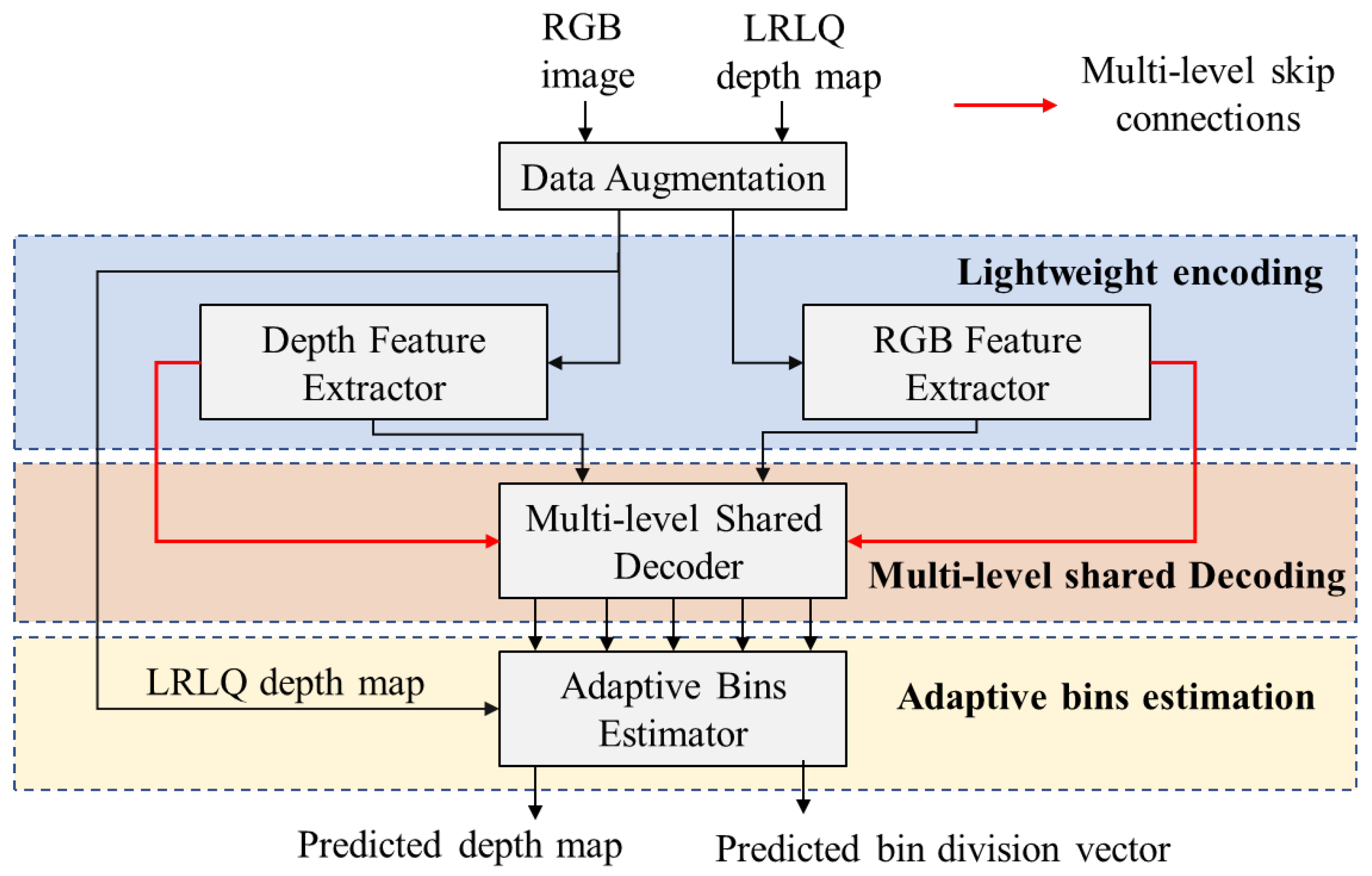
In the proposed depth estimation network, the inputs captured by MR glasses are RGB images and low-resolution low-quality (LRLQ) depth maps. The RGB image and the corresponding LRLQ depth map are fed into the feature extractors to extract their high- and low-level features separately. Those encoded features of image and depth are fused as multilevel dense depth features in a multilevel shared decoder. The multilevel shared decoder then decodes these dense features at different levels as the inputs of an adaptive bin estimator, as Figure 1 shows. The adaptive bins estimator conducts the prediction of bin divisions, which can delineate the depth distributions of current scenes. As a result, each high-resolution depth can be resulted from the linear combination of centers of divided bins with the bins’ probabilities. In our proposed network, the division of bins is hereafter named the bin-division vector, which contains the consecutive bins where a bin records the granularity (range) of a depth fragment.

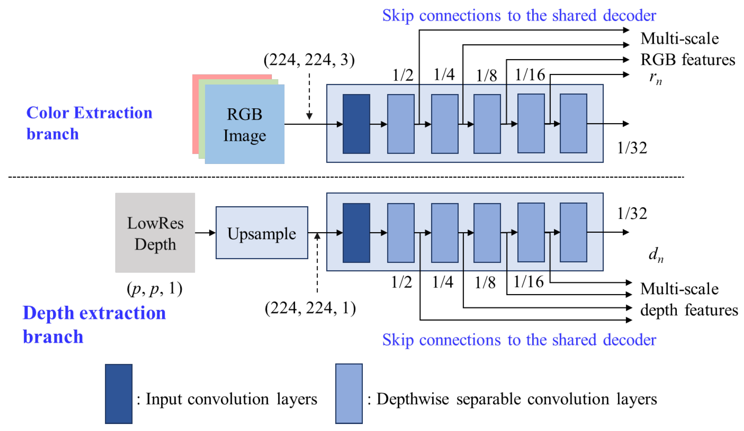
3.1. Lightweight Encoder

The proposed encoder is designed as a lightweight dual-path feature extractor where one path is called the RGB extraction branch and another is called the depth extraction branch, as shown in Figure 2. Their backbones with MobileNet-s can provide the multi-scale input features for the multi-level shared decoder. The inputs of the proposed encoders are the RGB image with a size of 224 × 224 × 3 and the LRLQ depth map with a size of p × p × 1, where p = 8 is set for the Jorjin J7EF Plus AR glasses [19]. The HR RGB image and LRLQ depth map are fed into the color extraction branch and depth extraction branch, respectively, so that the LRLQ depth maps are bi-linearly interpolated to the same spatial dimension as the RGB images before being fed into depth extraction branch.

For low-cost MR glasses, the primary consideration of designing modules should be high efficiency in computation. Inspired by FastDepth [10], we adopt MobileNet [30] with depthwise separable convolution layers as our feature extractors since they provide extreme computational efficiency. Then, we reduce the convolution layers on the original MobileNet layers to further achieve higher model throughput. The reduced encoder contains 6 depthwise separable convolution layers which can be regarded as a simplified MobileNet module, named MobileNet-s. The multilevel outputs of MobileNet-s are fed forward to the multilevel decoder through multilevel skip connections to generate the fused multilevel decoding features.

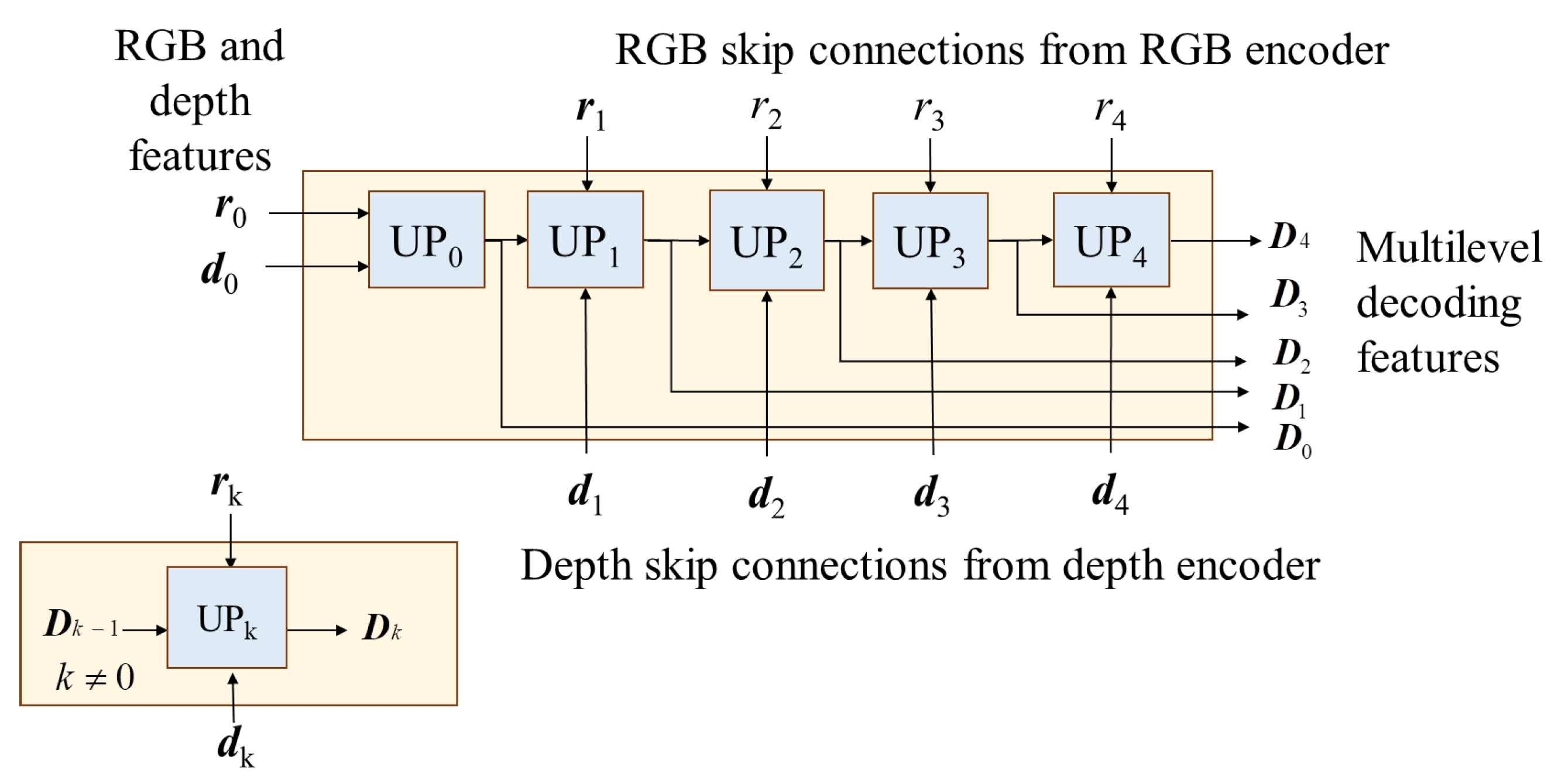
3.2. Multilevel Shared Decoder

In the multilevel shared decoder, the multi-scale depth and RGB features are separately inputted from the skip connections of the depth and RGB encoders. The multilevel shared decoder can sufficiently blend the RGB and depth features with five cascading upsample blocks, i.e., UP₀, UP₁, UP₂, UP₃ and UP₄, as shown by Figure 3. The nth upsample block (UP_n) gathers the nth level features r_n and d_n, which come from the RGB and depth branches, to generate the nth decoding depth feature termed D_n from D_n−1. Thus, the multilevel shared decoder iteratively generates multilevel decoding features, i.e., D₀, D₁, D₂, D₃ and D₄, and sends them in parallel to the adaptive bin estimator.

In this study, two types of upsampling blocks are designed to cover different application scenarios, which are named SimpleUp for high efficiency and UpCSPN-k for high-accuracy applications.

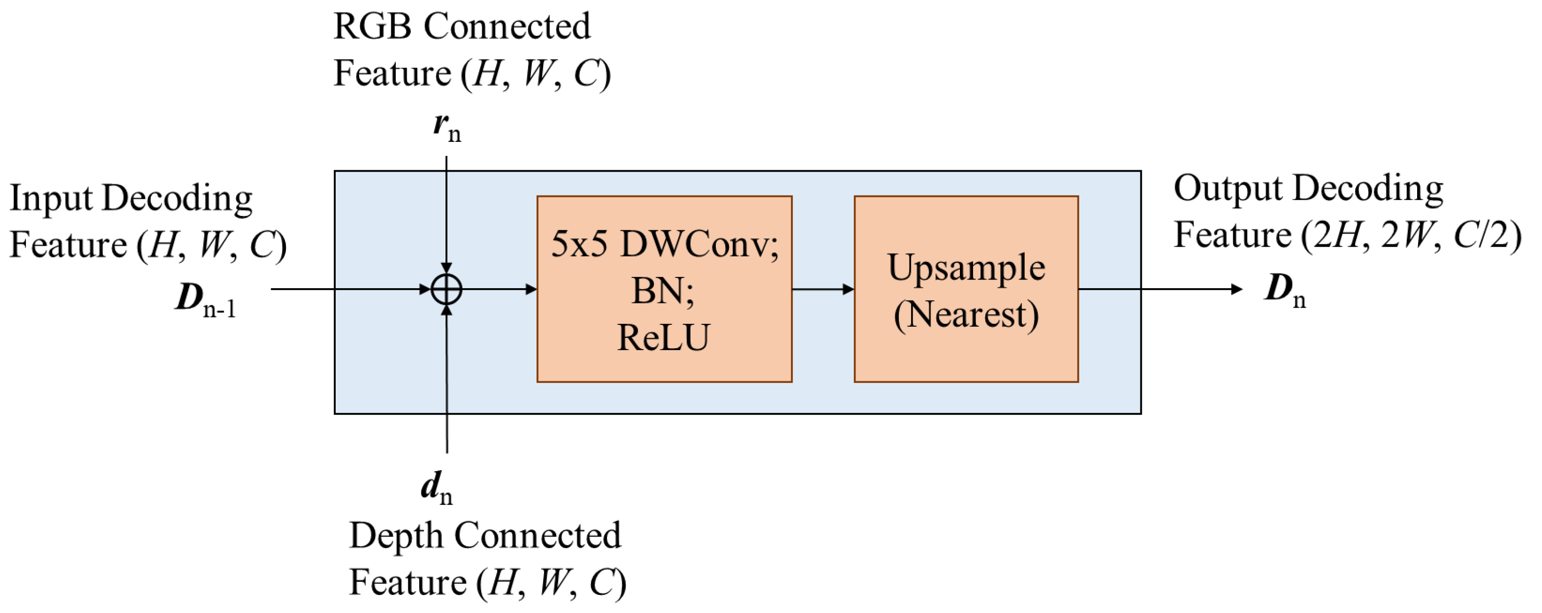
3.2.1. Upsampling by SimpleUp

For applications in low-resource apparatuses and mobiles, the design of the upsampling block must be very lightweight to fit the restrictions of the target hardware. Therefore, we suggest a simple high-efficiency module for the upsampling block called SimpleUp. As shown in Figure 4, the encoding results r_n and d_n are blended with the last-level decoding result D_n−1 together in the nth upsampling block (UP_n) by element-wise addition. We adopt element-wise addition rather than concatenation, because concatenation will increase the channels of features and consume additional resources for the subsequent convolution operation. SimpleUp consists of a 5 × 5 convolution kernel to reduce the channel number by half followed by bilinear interpolation to double the spatial resolution at each layer. In the convolution layers of SimpleUp and UpCSPN-k, depthwise separable convolution is adopted over standard convolutions to further reduce the parameters of the decoding layers. At the beginning of SimpleUp and UpCSPN-k, element-wise addition is applied to blend the RGB features and depth features. In Figure 3 and Figure 4, the first decoding result D₀ of the multilevel shared decoder has 512 channels, i.e., C = 512.

3.2.2. Upsampling by UpCSPN-k

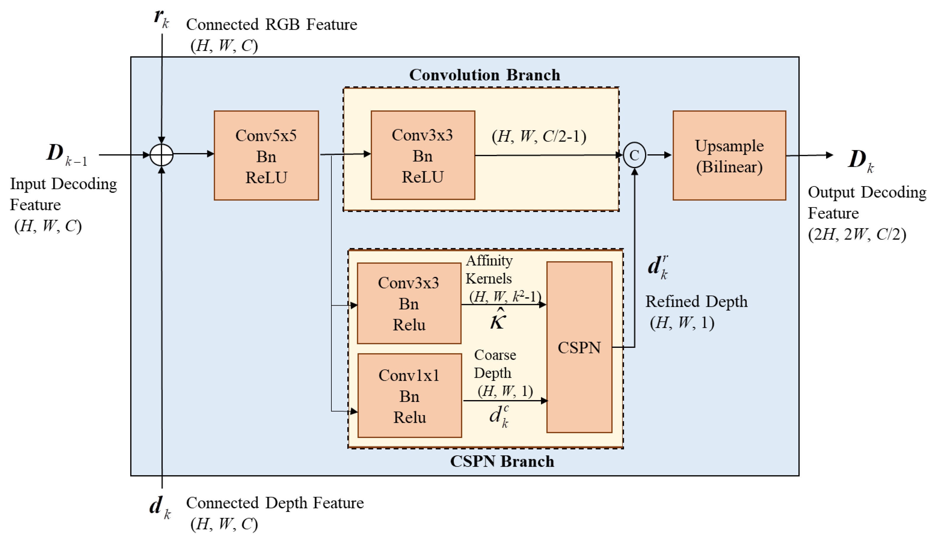
With relatively adequate resources, a complexity-moderate upsampling module called UpCSPN-k can be selected for high-accuracy applications. UpCSPN-k utilizes CSPNs over the layers of the decoder to iteratively produce the refined depths. As shown in Figure 5, the input RGB feature r_n and depth feature d_n with a size of (H, W, C) in the nth layer are passed through a 5 × 5 convolution then divided into two branches, the convolution branch and the CSPN branch.

In Figure 5, the convolution branch performs one 3 × 3 standard convolution with batch normalization to output features of size (H, W, C/2-1). Meanwhile, the CSPN branch is composed of two prediction heads, which produce a coarse depth map $d_n^c$ with a size of (H, W, 1) and a predicted affinity map $\widehat{\kappa }(x)$ with a size of (H, W, k²-1), where k is the kernel size of the CSPN. For each pixel x in $\widehat{\kappa }(x)$, the convolution weights of the channels can help to convey the information of pixels through the spatial average.

Thus, the refined depth $d_n^r$ through CSPN processing in each decoding layer can be obtained as

$$d_x^r={\kappa }_x\left(x\right)\odot d_x^c+{\displaystyle \sum _{x_n\in {\mathcal{N}}_x}{\kappa }_x\left(x_n\right)}\odot d_{x_n}^c,$$

(1)

where x denotes the pixel indices, x_n denotes the local neighborhood N_x around x and “$\odot$” is the element-wise production. The refined affinity of x is given as

$${\kappa }_x\left(x\right)=1-{\displaystyle \sum _{x_n\in {\mathcal{N}}_k}{\kappa }_x\left(x_n\right),}$$

(2)

where the normalization of the predicted affinity map $\widehat{\kappa }(x)$ is performed by

$${\kappa }_x\left(x_n\right)={\widehat{\kappa }}_x\left(x_n\right)/{\displaystyle \sum _{x_n\in {\mathcal{N}}_x}\left|{\widehat{\kappa }}_x\left(x_n\right)\right|}.$$

(3)

After CSPN processing, the refined depth is concatenated with the features of the convolution branch, and then the spatial resolution of the concatenated results is doubled by a bilinear interpolator for each decoding layer. Although the upsampling of UpCSPN-k is more complex than that of SimpleUp, it can provide much more precision than SimpleUp.

Note that, instead of general convolution and concatenation, the element-wise addition and depthwise separable convolution in SimpleUp and UpCSPN-k can efficiently fuse due RGB features and depth features without performance degradation through extensive testing.

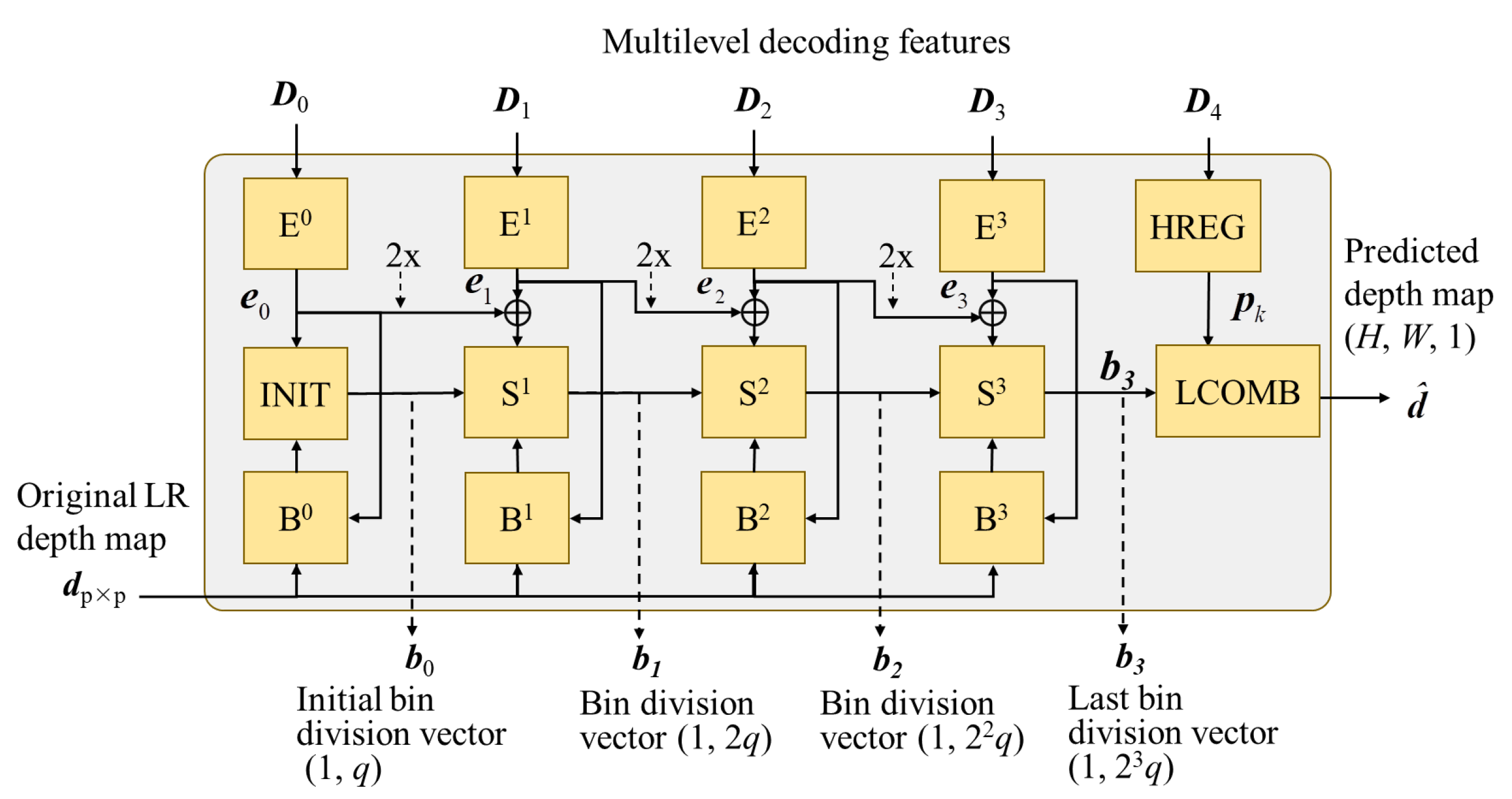
3.3. Adaptive Bin Estimator

After performing multilevel shared decoding, the multilevel decoding features, D₀, D₁, D₂, D₃ and D₄ are sent to the proposed adaptive dynamic-range bin (AdaDRBins) estimator. The AdaDRBins estimator employs these multilevel decoding features and the original LRLQ depth map, d_pxp, to produce the bin division patterns, i.e., the set of bin-division vectors {b₀, b₁, b₂, b₃} and the finally predicted depth map $\widehat{d}$, as Figure 6 shows. The ith component (i.e., the ith bin) of nth bin-division vector, b_n, is hereafter denoted by $b_n^i$.

The AdaDRBins estimator consists of four types of multiple layer perceptron (MLP): feature-embedding MLP (E_k-symbolized block), bin-initialization MLP (INIT-symbolized block), bin-splitter MLP (S_k-symbolized block) and bias-prediction MLP (B_k-symbolized block). Those MLPs exploit the individual fully connected (FC) structures to project the data into the different specified dimensions. The combination of those cascaded MLPs can make the dividing bins gradually be of a satisfactory fine granularity. The complete structures and signal flows of all MLPs are exhibited in Figure 7.

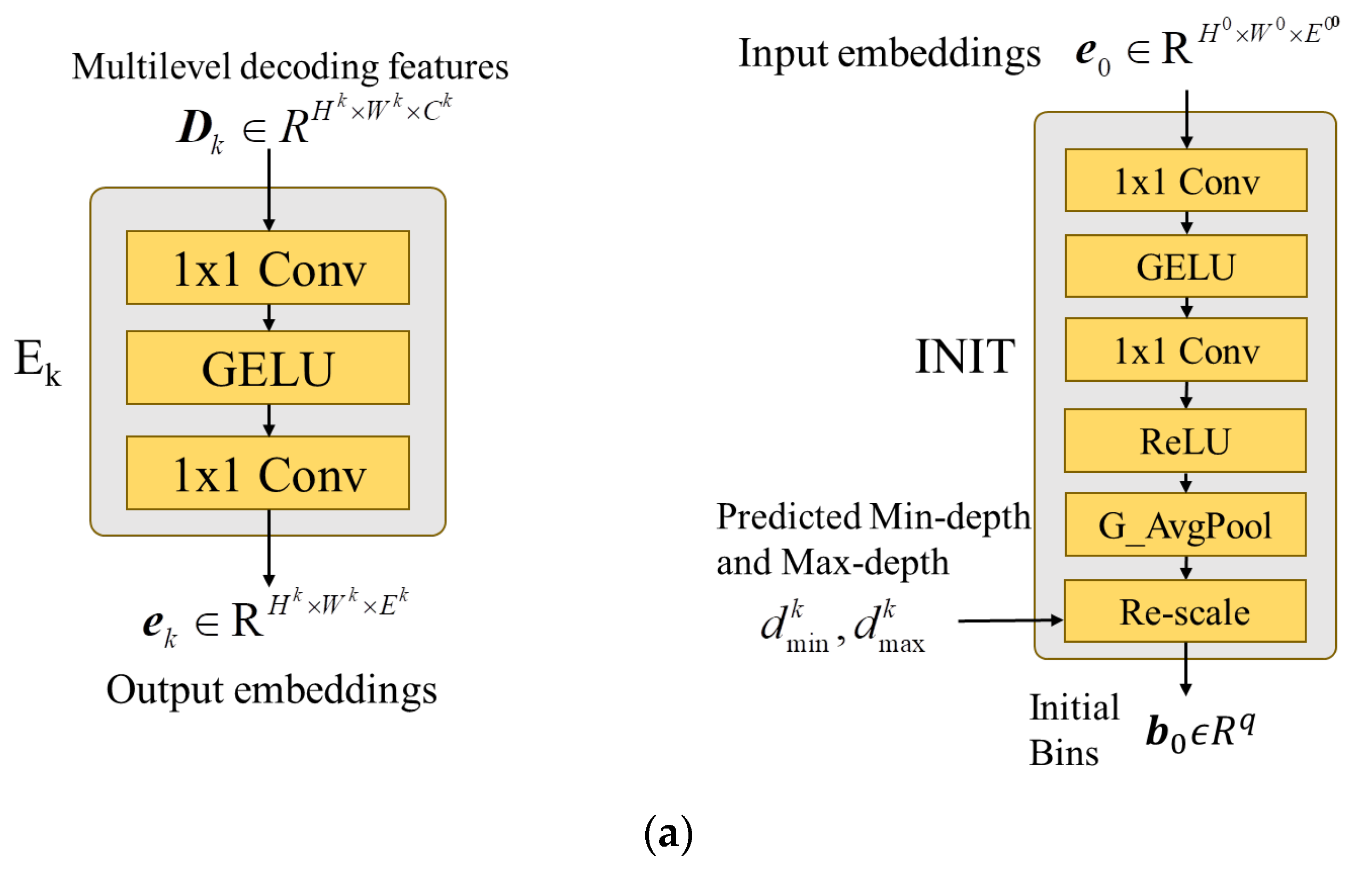
3.3.1. Feature-Embedding MLPs (E_n)

The decoded features are first passed through feature-embedding MLP layers. The embedding MLPs project the nth decoding features D_n with a size of (H_n, W_n, C_n) to become the nth embedding features, e_n, with a size of (H_n, W_n, C_e). The channel dimension C_e of embedding features now become the same size, which is referred to as “embedding space”.

Table 1. Details of feature-embedding MLPs while keeping the same H_n and W_n.

Layer Type	Input Channels	Output Channels	Activation
FC	Cn	64	GeLU
FC	64	Ce = 32	-

shows the detailed architecture of feature-embedding MLPs, where the proper channel dimension is assigned by C_e = 32 in our experiments. The subsequent layers within the AdaDRBins module utilize these embedding features to determine the appropriate bin division for each video frame.

3.3.2. Bin-Initialization MLPs (INIT)

The input of INIT is the first embedding feature denoted by e₀, which is obtained from the bottleneck of the decoder. INIT generates an initial bin-division vector, which is treated as coarse bin division to be the starting point of refining the bin division. This type of MLP generates an initial bin-division vector b₀ $\in$ R^q, where q is the initial number of bins. b₀ is viewed as the most coarse bin-division vector, and q is set as 4 through our extensive trials. In the subsequent bin-estimating layers, each bin will be consecutively split into two new bins layer by layer. For fitting the range of training datasets, the bins of the initial bin-division vector b₀ need to be re-scaled via normalization. The rescaling can be realized by renewing the centers of bins in b₀ by

$$c\left(b_0^i\right)=d_{\min }^0+\left(d_{\max }^0-d_{\min }^0\right)\cdot \left({\overline{b}}_0^i/2+{\displaystyle \sum _{j=1}^{i-1}{\overline{b}}_0^j}\right), i=0,1,\dots (q-1)$$

(4)

where $c\left(b_0^i\right)$ is the center depth of $b_0^i$ and ${\overline{b}}_0^j=b_0^j/\left|b_0\right|=norm\left(b_0^j\right)$ is the normalized jth bin in b₀; $d_{\min }^0$ and $d_{\max }^0$ denote the predicted minimal depth and maximal depth of bias prediction MLP, B₀, respectively.

Table 2. Details of INIT MLPs while keeping the same H_n and W_n.

Layer Type	Input Channels	Output Channels	Activation
FC	32	64	GeLU
FC	64	q	RLU
Global AvgPool	-	-	-

shows the detailed architecture of INIT MLPs.

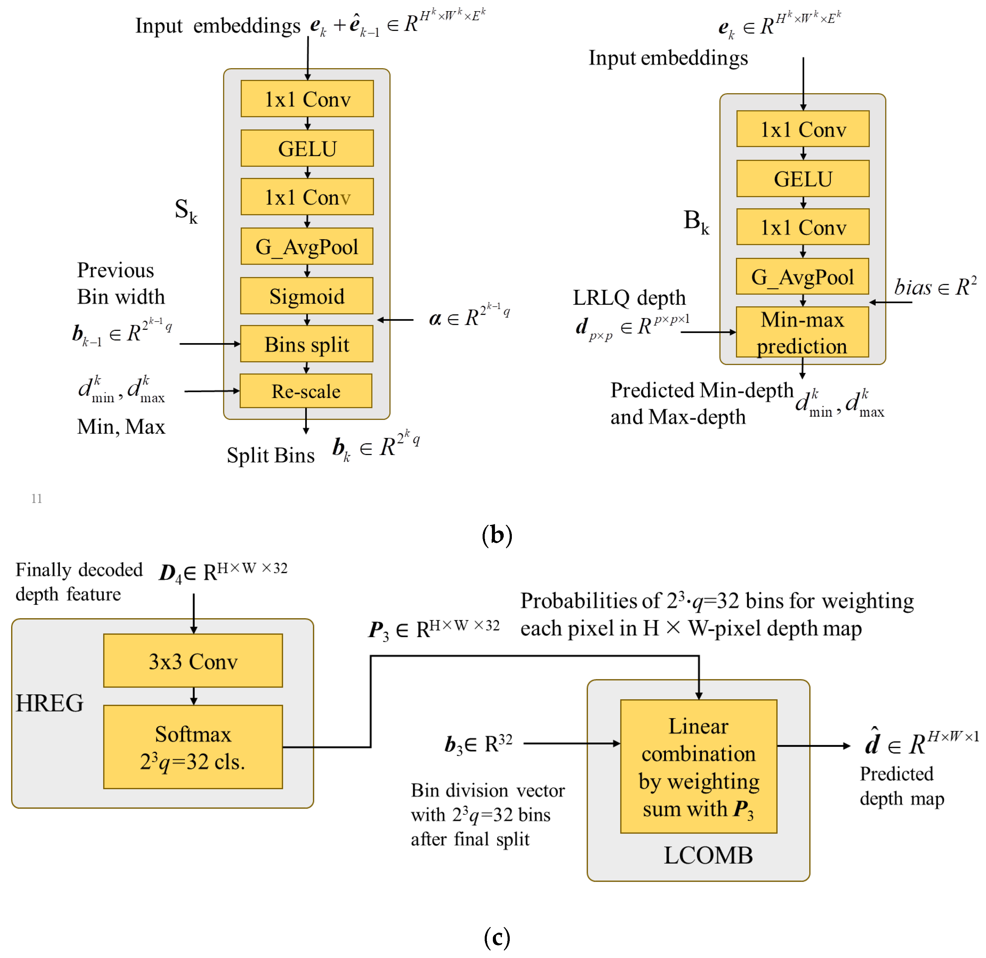
3.3.3. Bin-Splitter MLPs (S_n)

After bin initialization, the initial bin division is sent to the bin-splitter MLPs to perform the coarse-to-fine bin generation strategy. The bin-splitter MLPs play an important role in determining the distribution of bins, based on their respective bin embeddings. In essence, they act as decision-makers to determine how the previous bin division should be divided for improving the precision and the resolution of bins. As shown in Figure 6, the interpolated embedding features of the previous layer are element-wisely added with the embedding features of the current layer and then fed into the next bin-splitter MLP. After the FC layer in each bin-splitter MLP, the features are passed through a sigmoid activation function to obtain a split score vector of dimension $2^{(n-1)q}$ denoted by $\alpha =\left[{\alpha }^0,{\alpha }^1,\dots ,{\alpha }^{(2^{n-1}q-1)}\right]$. The scores in this vector determine how each previous bin is divided into two bins. The bin-splitter MLP imposes the nth bin division on b_n−1 with $\alpha$ to obtain the bin-division vector the nth bin-division vector b_n as

$$b_n=\left[{\alpha }^0{b}_{n-1}^0,\left(1-{\alpha }^0\right)b_{n-1}^0,{\alpha }^1{b}_{n-1}^1,\left(1-{\alpha }^1\right)b_{n-1}^1,\dots ,{\alpha }^{(2^{n-1}q-1)}{b}_{n-1}^{(2^{n-1}q-1)},\left(1-{\alpha }^{(2^{n-1}q-1)}\right)b_{n-1}^{(2^{n-1}q-1)}\right].$$

(5)

This binning processing increases granularity and resolution as the layers progress, ultimately improving the quality of the output. Similar to INIT, the bins of the output bin-division vector are re-scaled by the renewing their centers to fit the depth range of the training dataset, given by

$$c\left(b_n^i\right)=d_{\min }^n+\left(d_{\max }^n-d_{\min }^n\right)\cdot \left({\overline{b}}_n^i/2+{\displaystyle \sum _{j=1}^{i-1}{\overline{b}}_n^j}\right),i=0,1,\dots ,(2^{n}q-1),$$

(6)

where $d_{\min }^n$ and $d_{\max }^n$ are the predicted minimal depth and maximal depth of bias-prediction MLP B_n.

Table 3. Details of the nth splitting MLPs while keeping the same H_n and W_n.

Layer Type	Input Channels	Output Channels	Activation
FC	32	64	GeLU
FC	64	2n−1·q	-
Global AvgPool	-	--	-

details the architecture of the nth splitting MLPs.

3.3.4. Bias-Prediction MLPs (B_n)

For low-resolution depth inputs, we only have a rough understanding of the depth distribution in the scene. Our general idea is to constrain the predicted depth range, making the bin prediction closer to the GT depth range. Since the minimum and maximum depths in a low-resolution depth map may not be identical to the true minimum and maximum depths in ground truth, a bias term is needed for compensating the predictive offset. The bias MLP consists of two inputs: the low-resolution depth map d_pxp and the embedding feature e_n. The outputs are the estimated minimum depth and maximum depth of the scene. The embedding feature is passed through a bias-prediction MLP to estimate the minimum and maximum depths. The estimated biases are added to the minimum value and maximum value of ${\mathit{d}}_{p\times p}$ to obtain $d_{\min }^n$ and $d_{\max }^n$ given by

$$d_{\mathrm{m}\mathrm{i}\mathrm{n}}^n=\mathrm{m}\mathrm{i}\mathrm{n}\left({\mathit{d}}_{p\times p}\right)+bia{s}_{\mathrm{m}\mathrm{i}\mathrm{n}}^n\mathrm{and} d_{\mathrm{m}\mathrm{a}\mathrm{x}}^n=\mathrm{m}\mathrm{a}\mathrm{x}\left({\mathit{d}}_{p\times p}\right)+bia{s}_{\mathrm{m}\mathrm{a}\mathrm{x}}^n,$$

(7)

where $bia{s}_{\mathrm{m}\mathrm{i}\mathrm{n}}^n$ and $bia{s}_{\mathrm{m}\mathrm{a}\mathrm{x}}^n$ are, respectively, the predicted minimum and maximum biases generated by the bias prediction of B_n.

The predicted minimum depth and maximum depth are then fed into the bin-initialization MLP and bin-splitter MLP with the more accurate dynamic depth range of the current scene.

Table 4. Details of the nth bias MLPs while keeping the same H_n and W_n.

Layer type	Input Channels	Output Channels	Activation
FC	32	32	GeLU
FC	64	2	-
Global AvgPool	-	--	-

details the architecture of the nth bias MLPs.

3.3.5. Hybrid Regression Layer (HREG) and Linear Combination (LCOMB)

The final stage in the AdaDRBins estimator is the hybrid regression layer (HREG) and linear combination (LCOMB), which are detailed in Figure 7c. After the prediction of these MLPs, the final bin-division pattern b₃ is obtained. In the final stage of AdaDRBins, HREG is used on the final decoded feature D₄ to estimate the probabilities of each pixel falling into these bins. The hybrid regression layer consists of a 3 × 3 convolution followed by a Softmax activation unit, which results in the predicted probability p_i for the ith bin. Then, the predicted probabilities are applied to perform LCOMB with the predicted final centers of the bins $c\left(b_3^i\right)$, which are given by

$$c\left(b_3^i\right)=d_{\min }^3+\left(d_{\max }^3-d_{\min }^3\right)\left(b_3^i/2+{\displaystyle \sum _{j=1}^{i-1}{b}_3^j}\right),$$

(8)

for achieving the final predicted depth map $\widehat{d}$. The predicted depth at (x, y) in $\widehat{d}$ can be obtained by

$$\widehat{d}(x,y)={\displaystyle \sum _{i=1}^{N}c}\left(b_3^i\right)p_i(x,y),$$

(9)

where p_i(x, y) is the probability of predicted depth at (x, y) falling in the ith bin, where N is 2³·q = 32.

3.4. Loss Functions

Similar to AdaBins [12], we employ two loss terms to assemble the loss function, which is designed as

$${\mathcal{L}}_{total}=\beta {\mathcal{L}}_{reg}+\mu {\mathcal{L}}_{bins},$$

(10)

where ${\mathcal{L}}_{reg}$ and ${\mathcal{L}}_{bins}$ denote the per-pixel regression loss and bin center distribution loss, respectively. Through extensive examinations of AdaDRBins, the scaling factors β = 10 and μ = 0.5 are selected because they can attain higher accuracy of depth estimation, on average, and achieve more training for our proposed network than other tested values of β and μ.

3.4.1. Scale-Invariant Log Loss

We use masked scale-invariant log (SILog) loss proposed by Eigen et al. [5] as the per-pixel regression loss. The loss term is defined by

$${\mathcal{L}}_{reg}=\sqrt{{\displaystyle \frac{1}{N}}{\displaystyle \sum _i{g}_i^2}-{\displaystyle \frac{\lambda }{N^2}}{\left({\displaystyle \sum _i{g}_i}\right)}^2},$$

(11)

with

$$g_i=\log d_i-\log {\widehat{d}}_i,$$

(12)

where $d_i$ and ${\widehat{d}}_i$ denote GT depth and predicted depth at pixel i, respectively, and N denotes number of valid pixels in GT depth (i.e., $d_i>0$). Similar to AdaBins, we set λ = 0.85 in our experiments.

3.4.2. Bin Center Distribution Loss

Similar to primary AdaBins, the chamfer distance [31] is adopted as the bin center distribution loss in order to supervise the distribution of predicted bin centers. Let ${\mathcal{C}}_{pred}=\left\{c_1,c_2,c_3,c_4\right\}$ denote the set of predicted bin centers at different scales and $d_{gt}\in {\mathrm{R}}^{HW}$ denote the set of valid GT values. The loss term is given by

$${\mathcal{L}}_{bins}={\displaystyle \sum _{b\in \mathcal{B}}CD}\left(c,d_{gt}\right),$$

(13)

where the chamfer distance is defined as

$$CD(X,Y)={\displaystyle \frac{1}{\left|X\right|}}{\displaystyle \sum _{x\in X}\underset{y\in Y}{\min }}‖x-y‖+{\displaystyle \frac{1}{\left|Y\right|}}{\displaystyle \sum _{y\in Y}\underset{x\in X}{\min }}‖x-y‖.$$

(14)

This loss term promotes the alignment between the distribution of bin centers and the distribution of GT depth values by pushing the bin centers to match the actual depth values, on average.

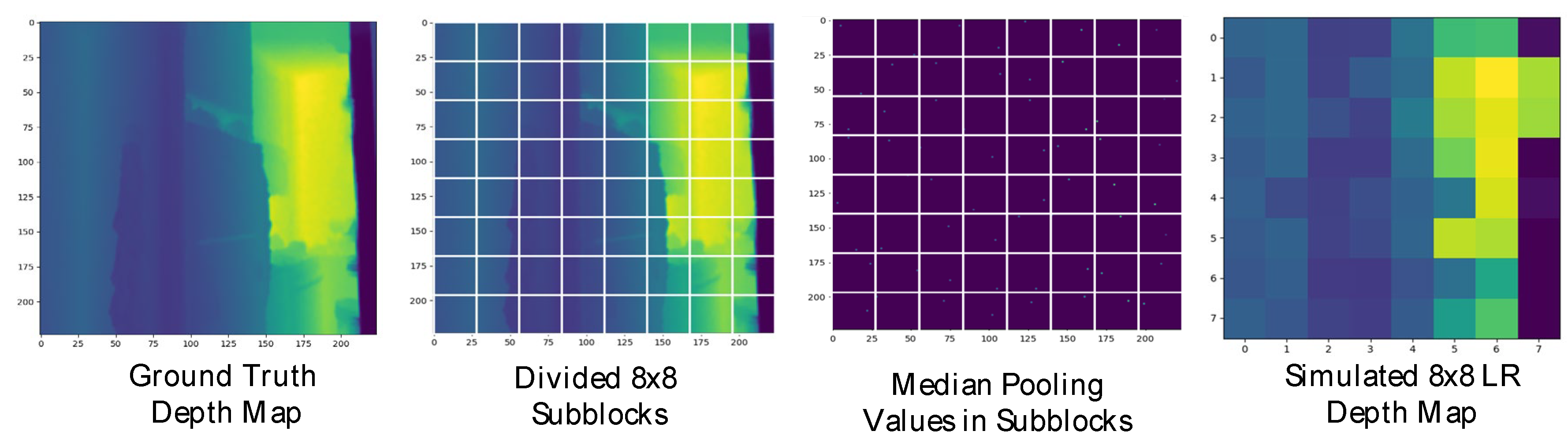
3.5. LRLQ Depth Generation for Training

In order to simulate the LRLQ depth maps obtained from MR glasses for training, we introduce a depth sampling method that generates low-resolution depths randomly from the ground truth. Figure 8 shows the results of LRLQ depth generation with p = 8 by our proposed simulation strategy, where the proposed two-step LRLQ depth generation is stated as follows:

Step 1. 

Subblocking: To obtain a p × p low-resolution depth map $d_{p\times p}$ from the GT depth map d, we first divide the GT depth map into p × p subblocks.

Step 2a. 

Median pooling: We simply take the median value of each sub-block as the LP depth value to obtain the simulated LRLQ depth map.

Step 2b. 

Max-depth filtering (optional): In practice, the depth range on most MR glasses’ depth sensors is limited to a short distance range. To simulate the short distance range depth during training, we apply max-depth filtering on the sampled low-resolution depth map. As the depth value is greater than a max-depth threshold, max-depth filtering will reset the depth value to zero (i.e., invalid pixel).

4. Experimental Results

In this section, we will first describe the datasets and implementation settings. Then, we will exhibit the depth estimation performance achieved by the proposed network in various evaluation criteria.

4.1. Datasets and Implementation Settings

We used the NYU Depth V2 dataset [32] and EgoGesture dataset [33] as our training datasets. NYU Depth V2 provides pairs of RGB images and the corresponding depth map for indoor scenes. The image and depth map resolution of the dataset were captured at 640 × 480 from Microsoft Kinect, which renders a maximum sensible distance of 10 meters. We employed the official train/test split in our experiments, which comprises 12,000 training samples and 654 testing samples. The EgoGesture dataset provides RGB images and the depth map of diverse hand gestures. The dataset was gathered by Intel RealSense SR300 with a resolution of 640 × 480. The dataset encompasses four indoor scenes and two outdoor scenes. In total, the dataset contains 2,953,224 hand gesture frames collected for the RGB and depth modality, respectively.

Our experiments were implemented with Python 3.9, PyTorch 1.10.2 [34], CUDA 11.3 and cuDNN 8.2 on the Ubuntu 22.04 LTS operating system. We trained our network using a single NVIDIA GeForce RTX 4090 GPU with 24 GB of memory and an Intel i7-13700K CPU. During training, we utilized a batch size of 16 and an Adam [34] optimizer with (0.95, 0.99) betas and 0.1 weight decay. The proposed depth estimation network is trained over 50 epochs with the learning rate starting from 0.000357 and decaying 20% every 5 epochs.

4.2. Proposed Network Implementation on Low-Cost MR Glasses

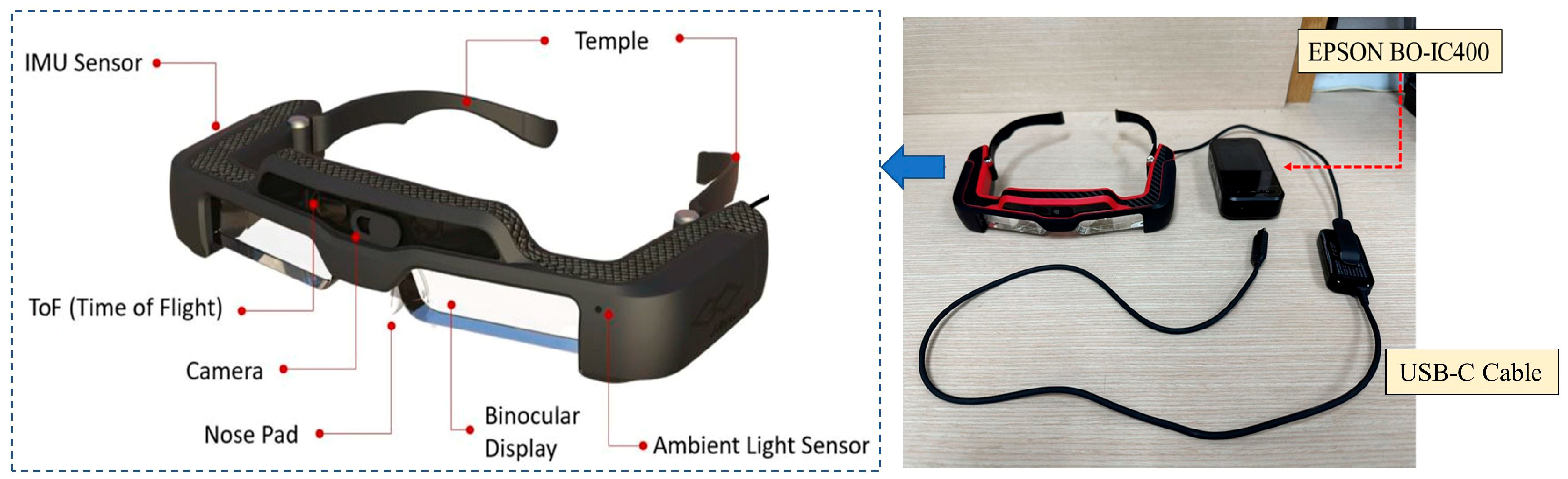
The profile and components of Jorjin J7EF Plus AR glasses are described by Figure 9, which contains two major parts: an MR goggle with several sensors and a computation device connected through a USB type C connector. There are several useful sensors built on this MR goggle, including a time-of-flight (ToF) sensor, an RGB camera, a gyroscope, an accelerator and a magnetometer. The resolution of the ToF sensor is 8 × 8 and its sensing distance range is roughly within 3 meters, which is comparably low. Our goal is to utilize the LRLQ depth map and RGB images from Jorjin’s MR glasses to obtain a precise and high-resolution depth map by using the EPSON BO-IC400 platform [35], which adopts a Qualcomm SXR1130 processor with 4 GB memory and 64 GB storage.

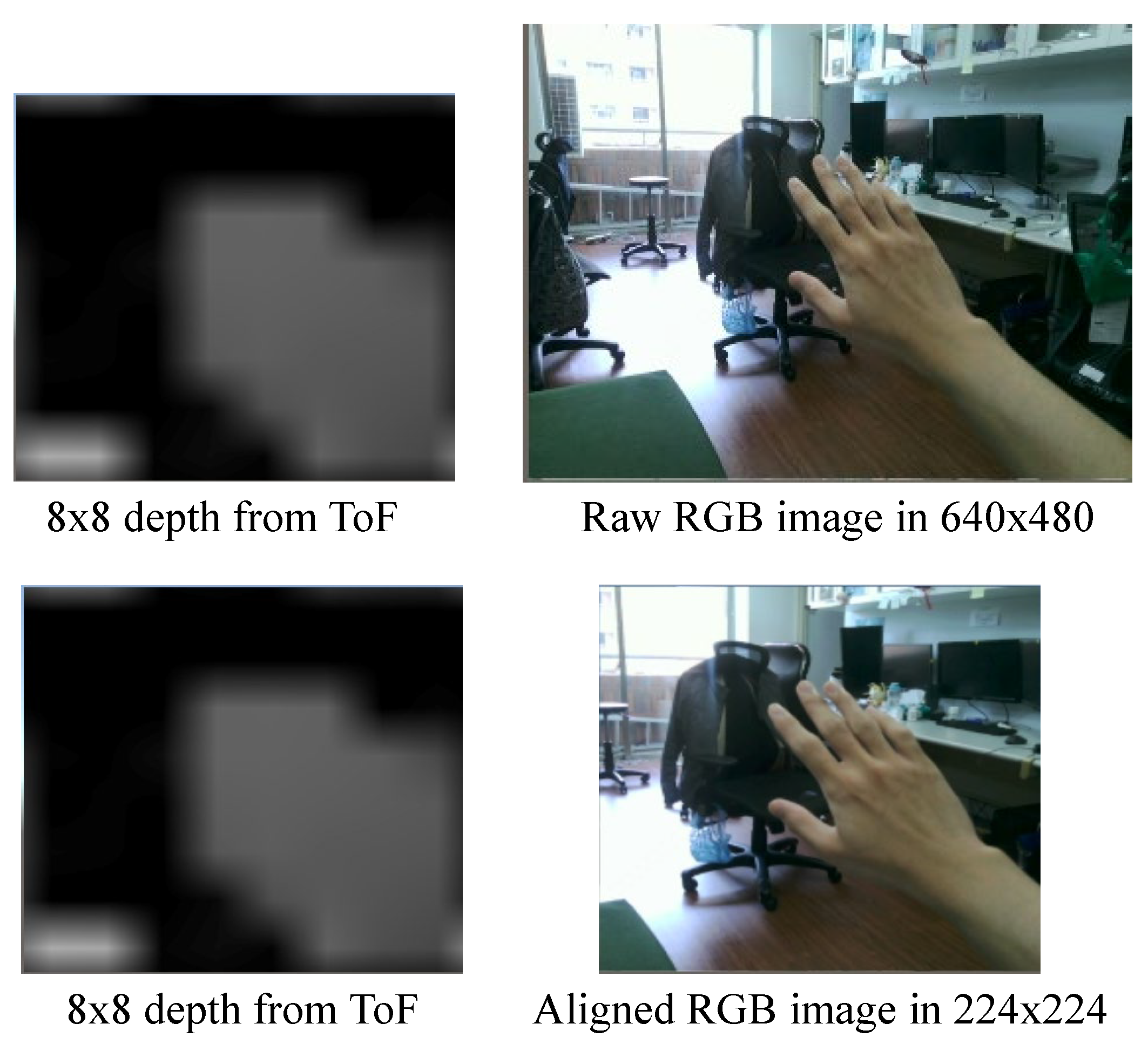
For the Jorjin AR glasses sensor, the resolutions of captured raw RGB images and depth maps are 640 × 480 and 8 × 8, respectively. Since the spatial positions of RGB and depth images must be fully aligned, we first resize the raw RGB image into 360 × 270 and crop the region RGB_crop = {(x, y): 68 ≤ x ≤ 191, 23 ≤ y ≤ 246} to make the cropped color images be 224 × 224 RGB images for further alignment with depth maps. We tried the spatial transformer network to align the RGB and depth images. However, this deep learning network not only consumes additional costs but also causes some unpredictable inaccuracies in the alignment. Hence, we adopt a semi-automatic alignment by the aid of easy manual refinement. An alignment result for Jorjin MR glasses data is displayed by Figure 10. Because the calculation of depth-estimation loss directly exploits the high-resolution GT depth maps provided by the NYU Depth V2 dataset and EgoGesture dataset, those high-resolution GT depth maps are downsampled as sensor-labeled 8×8 depth maps for training the models of our network.

For verifying the feasibility of our model for resource-limited MR glasses, we implement the simplest model with the sole-SimpleUp decoder w/o AdaDRBins. Unity with version 2020.3.29f1 is used as our engine to build the virtual scene on MR glasses. Jorjin provided the software development kit (SDK) for MR glasses on Unity, and we can access the MR sensor data with Unity scripting API in C# language. We use Barracuda Unity 3.0.0 as our model inference library. Barracuda Unity provides a lightweight and cross-platform neural network inference API for Unity. It can inference neural networks in ONNX (Open Neural Network Exchange) format directly on both the CPU and GPU of supported platforms.

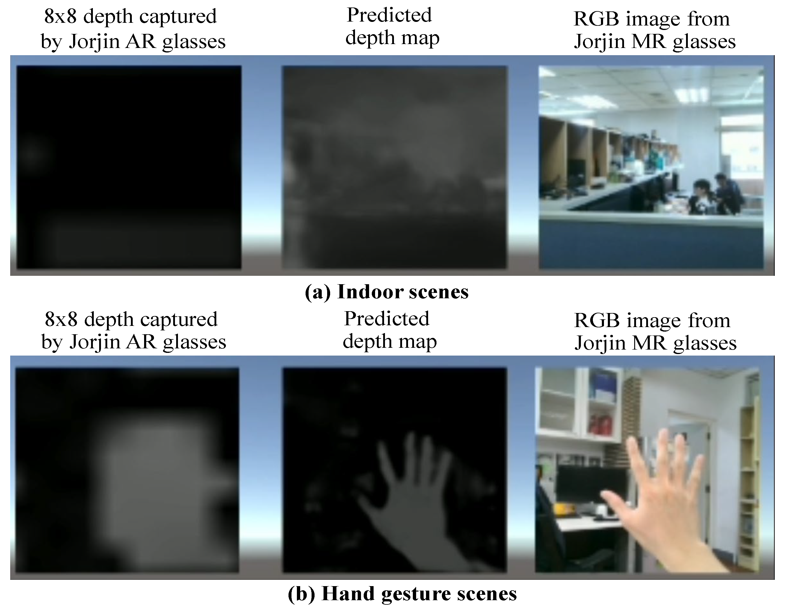
For indoor scenes, the model is trained on the NYU Depth V2 dataset, and we apply max depth filtering of 3 meters on the depth training samples. For handling the gesture scenes, the model is trained on the EgoGesture dataset and we apply max depth filtering of 1.5 meters on the depth training samples. Figure 11 displays the estimated high-precision depths for indoor and dynamic hand scenes on Jorjin MR glasses by the simplest model with only a SimpleUp decoder without AdaDRBins. There are three types of contents, 8×8 depths captured by the ToF sensor, the depth estimation result predicted by our proposed network and the RGB image captured by the Jorjin MR glasses. For the result of indoor scenes, we can see the network roughly understand the depth information of the scene. However, the depth sensing range of the MR glasses is very low. Hence, the image with far objects in the first row is unable to have a good predicted depth map. For hand gesture scenes, since the distance range of hand gestures can fit the short depth sensing range of the ToF sensor, the position and distance of a hand with dynamic gestures can be clearly identified. We believe that with the high-resolution depth information on MR glasses, many applications can be more accurate. To see the hand gesture demos in details, one can download Video S1, EgoGesture demo.mp4, at https://youtu.be/XFgtftdPQls, accessed on 1 August 2023.

4.3. Performance Evaluation Results

For the experiments, we adopt MobileNet-s as the encoder. We use the official testing split, which contains 654 testing samples, to test the performance by using average evaluation metrics. The resolution of RGB images is set to 224 × 224 and the resolution of simulated LRLQ depths is set to 8 × 8. We compare the proposed models to FastDepth [10] with ResNet50 + NNConv5, FastDepth [10] with MobileNet + NNConv5 and MonoDepth [13] with ResNet50 + DispNet for 224 × 224 RGB input images. As

Table 5. Comparisons of FastDepth, MonoDepth and the various proposed variants by using the NYU Depth V2 dataset.

Network	Encoder	Decoder	Weights (M)	MAC (G)	RMSE
FastDepth [10]	ResNet50	NNConv5	25.60	4.190	0.568
FastDepth [10]	MobileNet	NNConv5	3.19	0.740	0.599
MonoDepth [13]	ResNet50	DispNet	30.00	4.800	>4.392
Proposed	DMobileNet_s	SimpleUp	2.18	0.675	0.223
Proposed	DMobileNet_s	SimpleUp+ AdaDRBins	2.28	1.150	0.199
Proposed	DMobileNet_s	UpCSPN-7+ AdaDRBins	43.57	9.445	0.185

shown, the FastDepth [10] with ResNet50+NNConv5 and the MonoDepth [13] with ResNet50 + DispNet respectively require about 0.74 G MACs and 4.8 G MACs for 224 × 224 depth map completion. In our proposed network, the Dual MobileNet encoder including six depthwise separable convolution layers and one pointwise convolution totally requires about 0.185G MACs. In Table 5, three proposed models using the solo-SimpleUp decoder, the SimpleUp + AdaDRBins decoder and the UpCSPN-7 + AdaDRBins decoder are chosen to display their computational complexities in order. These three models demand 0.675 (i.e., 0.185 + 0.49), 1.335 (i.e.,0.185 + 1.15) and 9.445 (i.e.,0.185 + 9.26) G MACs, respectively. The proposed simplest model, which adopts the solo-SimpleUp decoder, is not only lighter than the fastest version of FastDepth in MACs but also achieves a lower 0.233 RMSE than the 0.599 RMSE obtained for testing the NYU Depth V2 dataset. It is noted that MonoDepth tested on the KITTI dataset attains 4.392 RMSE in monotonous outdoor scenes. Thus, for the more complex indoor dataset, e.g., the NYU Depth V2 dataset, the RMSE of MonoDepth shall be larger than 4.392, such that we enlisted the RMSE of MonoDepth as “>4.392” in Table 5.

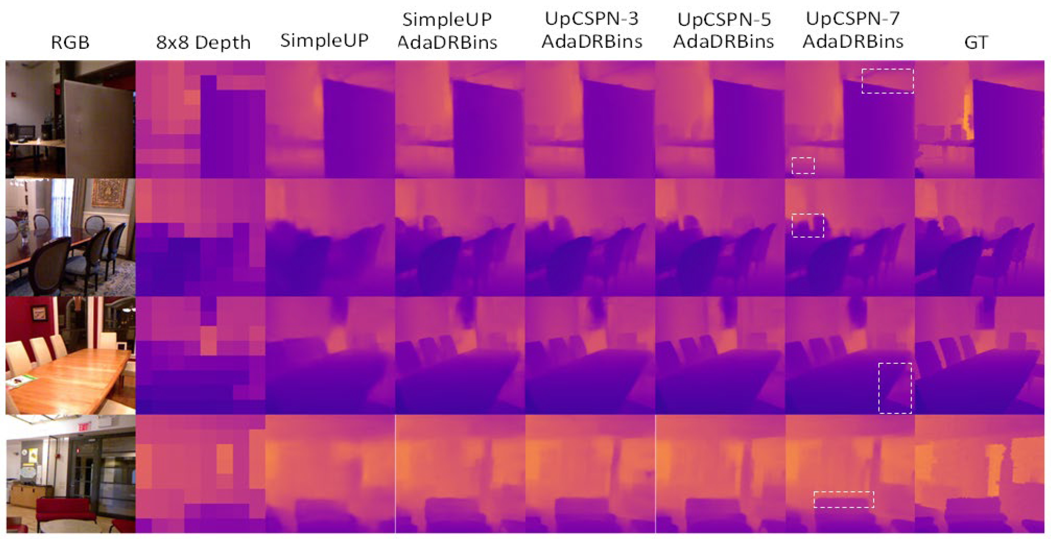
In Figure 12, the qualitative results of our proposed network on the NYU Depth V2 dataset are displayed in a visualization. We observe that the depth maps achieved by the combination of the UpCSPN-k and AdaDRBins modules preserve more details and clearer boundaries than those obtained by SimpleUp. However, the depth maps that resulted from the model with the solo-SimpleUp decoder are still clear and recognizable. For considering the balance of complexity and precision, the combination of SimpleUP and AdaDRBins could be a good solution for resource-limited platforms. Particularly, observing the second and fourth rows of Figure 12, the rectangle-highlighted depth areas resulting from the proposed network using UpCSPN-7 + AdaDRBins decoder can be even better than the corresponding depth areas in GT maps in terms of visual rationality.

Through our experiments, the depth completion accuracy of 32 bins is very close to those of 64 bins, 128 bins and 256 bins for 224 × 224 depth maps while adopting AdaDRBins in the proposed architecture. It means that the use of 32 bins provided by AdaDRBins, i.e., 32-bin AdaDRBins, could be the most appropriate under the consideration of model complexity for our proposed models. The computational complexity comparisons of 32-bin AdaDRBins and 256-bin AdaBins [12] are listed at

Table 6. The complexity comparisons of 32-bin AdaDRBins and 256-bin AdaBins [12] used in the proposed models for generating high-precision 224 × 224 depth maps.

Decoder	Bins Estimator	#Bins	Weights (M)	MAC (G)	FPS
SimpleUp	AdaBins	256	4.52	4.43	430
UpCSPN3	AdaBins	256	45.10	11.97	280
UpCSPN5	AdaBins	256	45.39	12.20	270
UpCSPN7	AdaBins	256	45.81	12.54	240
SimpleUp	AdaDRBins	32	2.28	1.15	560
UpCSPN3	AdaDRBins	32	42.86	8.70	340
UpCSPN5	AdaDRBins	32	43.14	8.92	330
UpCSPN7	AdaDRBins	32	43.57	9.26	310

.

4.4. Ablation Study

For the ablation study, we exhibit the quantitative metrics of the proposed networks with different amounts and complexities of ingredients in

Table 7. Quantitative results of the proposed networks achieved by different structures, where REL expresses the relative error and δ₁ = 1.25, δ² = 1.25² and δ³ = 1.25³ are the error-toleration thresholds of ratios of estimated depth and GT depth.

Decoder	Bins Estimator	RMSE (m)	REL	${\mathit{\delta }}_1$	${\mathit{\delta }}_2$	${\mathit{\delta }}_3$
SimpleUp	--	0.223	0.046	97.36	99.43	99.85
UpCPSN-3	--	0.206	0.039	97.87	99.56	99.89
UpCPSN-5	--	0.197	0.036	97.87	99.55	99.89
UpCPSN-7	--	0.202	0.036	97.87	99.54	99.89
SimpleUP	AdaBins	0.197	0.037	98.04	99.64	99.91
SimpleUp	AdaDRBins	0.199	0.038	98.06	99.64	99.91
UpCSPN-3	AdaDRBins	0.190	0.036	98.21	99.67	99.92
UpCSPN-5	AdaDRBins	0.191	0.036	98.21	99.67	99.92
UpCSPN-7	AdaDRBins	0.185	0.034	98.24	99.67	99.92

and

Table 8. Computational analyses of the proposed networks with different structures where MAC expresses the number of multiply accumulated operations.

Decoder	Bins Estimator	#Bins	Weights (M)	MAC (G)	FPS
SimpleUp	--	-	2.18	0.49	1170
UpCPSN-3	--	--	41.85	8.04	367
UpCPSN-5	--	--	42.13	8.36	356
UpCPSN-7	--	--	42.57	8.60	337
SimpleUp	AdaBins	256	4.52	4.43	425
SimpleUp	AdaDRBins	32	2.28	1.15	560
UpCSPN-3	AdaDRBins	32	42.85	8.70	340
UpCSPN-5	AdaDRBins	32	43.14	8.92	330
UpCSPN-7	AdaDRBins	32	43.57	9.26	310

. The simulation results show that our simplest architecture of the decoder, i.e., Solo-SimpleUp, achieves comparable performance on NYU Depth V2 with incredibly fast inference speed, making it more suitable to be implemented on mobile devices.

Although the combinations of UpCSPN-k and AdaDRBins have lower inference speeds, their performances are much higher than the model with the solo-SimpleUp decoder. As Table 7 shows, the model with UpCSPN-7 and AdaDRBins can make the generated depth maps acquire very high precision with an RMSE of 0.185, which is lower the RMSEs achieved by existing AdaBin-based networks [12,21,22,23,24,25], i.e., with RMSEs higher than 0.19 for various task-specific testing images.

5. Discussion

In this study, for low-cost MR applications, we proposed depth estimation algorithms with lightweight encoders and a simpleUp multilevel shared decoder. The simplest network with only 2.18 M parameters was successfully implemented in Jorjin J7EF Plus AR glasses. It is noted that the proposed network with lightweight encoders, the UpCPSN-7 multilevel shared decoder and AdaDRbins, can achieve the highest precision performance in depth estimation, better than AdaBines-based networks.

We can divide the models of proposed network into four groups, whose decoders are “Solo-SimpleUp”, “UpCPSN-k only”, “SimpleUP + AdaxBins” (AdaxBins can be AdaBins and AdaDRBins) and “UpCSPN-k + AdaDRBins”. Observing Table 7, we find that the RMSEs of models between different groups have salient differences, and the RMSEs of models in the identical group have close RMSEs. Even that, in the second group, i.e., UpCPSN-k only, the “UpCPSN-5 only” decoder is better than the “UpCPSN-7 only” decoder. This fact can manifest as evidence for the deep learning investigation that more stacked layers could not guarantee better performance. We can claim that better structure design is more important than the use of larger amounts of kernels.

In this study, we follow the rule of gradually increasing the stacked ingredients and layers to develop our networks. The content of Table 6 can imply that the model with the “SimpleUP + AdaBins” decoder could be a teacher network to distill the model with the solo-SimpleUp decoder. Similarly, the model with the UpCSPN-l + AdaDRBins decoder can play a teacher role for the model using the UpCSPN-m + AdaDRBins decoder for l > m. Hence, based on this design strategy, the teacher-and-student structure can be easily attained by arbitrarily reducing the layers of a complex model for distillation. Observing Table 5, Table 6 and Table 8, the proposed model using MobileNet_s, SimpleUP and 32-bin AdaDRBins could be the best selection in real-time low-cost MR systems in terms of the efficiency–accuracy leverage.

Because the depths captured by the ToF depth camera in MR glasses are overly blurry, the original depths near fingers are mostly lost during hand-moving actions. The high-resolution depth predicted by our proposed networks can greatly support the accurate estimation of hand gestures in complex backgrounds. The predicted depths of finger pixels could provide a better foundation for the recognition of subtle 3D hand gestures. As a result, the proposed network has been acknowledged for facilitating surgery operations and surgical education/training by physicians affiliated with National Cheng Kung University Hospital. Hence, we believe that our proposed network will be an applicable edge-computing system for many other popular applications such as the detectors of self-driving vehicles and low-altitude drones with LR depth for real-time high-precision depth completion.

6. Conclusions

In this paper, the proposed low-complexity depth estimation network for obtaining high-precision depth maps contains dual-path encoders, multilevel variant shared decoders and adaptive dynamic-range bin estimators so that the decoders can sufficiently fuse the features of multiple scales delivered from the paths of encoding depths and RGB images. The models of the proposed networks are lightweight self-supervised high-precision depth estimators which can exploit an RGB image and a very blurry low-resolution depth map to generate high-precision high-dimension depth maps in resource-limited MR applications. In the proposed network, the most lightweight approach using MobileNet_s, SimpleUp and AdaDRBins only needs 2.28 M weights and 1.150 G MACs, which is very useful for the real-time recognition of hand gestures. Consequentially, the proposed network with various variants can be effectively deployed on mobile devices, MR glasses and AR apparatuses to render satisfactory depth maps under different clarity requirements and resource limitations.

References

- Fabrizio, F.; De Luca, A. Real-time computation of distance to dynamic obstacles with multiple depth sensors. IEEE Robot. Autom. Lett. 2017, 2, 56–63. [Google Scholar] [CrossRef]
- Kauff, P.; Atzpadin, N.; Fehn, C.; Müller, M.; Schreer, O.; Smolic, A.; Tanger, R. Depth map creation and image-based rendering for advanced 3DTV services providing interoperability and scalability. Signal Process. Image Commun. 2007, 22, 217–234. [Google Scholar] [CrossRef]
- Fehn, C. Depth-image-based rendering (DIBR), compression, and transmission for a new approach on 3d-tv. In Stereoscopic Displays and Virtual Reality Systems XI: 19–22 January 2004, San Jose, California, USA; SPIE: Bellingham, WA, USA, 2004; Volume 5291, pp. 93–104. [Google Scholar]
- Yang, W.-J.; Yang, J.-F.; Chen, G.-C.; Chung, P.-C.; Chung, M.-F. An assigned color depth packing method with centralized texture depth packing formats for 3D VR broadcasting services. IEEE J. Emerg. Sel. Top. Circuits Syst. 2018, 9, 122–132. [Google Scholar] [CrossRef]
- Natan, O.; Miura, J. End-to-end autonomous driving with semantic depth cloud mapping and multi-agent. IEEE Trans. Intell. Veh. 2023, 8, 557–571. [Google Scholar] [CrossRef]
- Suarez, J.; Murphy, R.R. Hand gesture recognition with depth images: A review. In Proceedings of the 2012 IEEE RO-MAN: The 21st IEEE International Symposium on Robot and Human Interactive Communication, Paris, France, 9–13 September 2012; pp. 411–417. [Google Scholar]
- Hirschmuller, H. Stereo processing by semiglobal matching and mutual information. IEEE Trans. Pattern Anal. Mach. Intell. 2007, 30, 328–341. [Google Scholar] [CrossRef]
- Eigen, D.; Puhrsch, C.; Fergus, R. Depth map prediction from a single image using a multi-scale deep network. In Advances in Neural Information Processing Systems; The MIT Press: Cambridge, MA, USA, 2014; pp. 2366–2374. [Google Scholar]
- Alhashim, I.; Wonka, P. High quality monocular depth estimation via transfer learning. arXiv 2018, arXiv:1812.11941. [Google Scholar]
- Wofk, D.; Ma, F.; Yang, T.-J.; Karaman, S.; Sze, V. Fastdepth: Fast monocular depth estimation on embedded systems. In Proceedings of the IEEE/CVF International Conference on Robotics and Automation (ICRA), Montreal, QC, Canada, 20–24 May 2019; pp. 6101–6108. [Google Scholar]
- Laina, I.; Rupprecht, C.; Belagiannis, V.; Tombari, F.; Navab, N. Deeper depth prediction with fully convolutional residual networks. In Proceedings of the IEEE International Conference on 3D vision (3DV), Stanford, CA, USA, 25–28 October 2016; pp. 239–248. [Google Scholar]
- Bhat, S.F.; Alhashim, I.; Wonka, P. Adabins: Depth estimation using adaptive bins. In Proceedings of the IEEE/CVF Conference on Computer Vision and Pattern Recognition, Nashville, TN, USA, 20–25 June 2021; pp. 4009–4018. [Google Scholar]
- Godard, C.; Aodha, O.M.; Brostow, G.J. Unsupervised monocular depth estimation with left-right consistency. In Proceedings of the IEEE Conference on Computer Vision and Pattern Recognition, Honolulu, HI, USA, 21–26 July 2017; pp. 270–279. [Google Scholar]
- Godard, C.; Aodha, O.M.; Firman, M.; Brostow, G.J. Digging into self-supervised monocular depth estimation. In Proceedings of the IEEE/CVF International Conference on Computer Vision, Seoul, Republic of Korea, 27 October–2 November 2019; pp. 3828–3838. [Google Scholar]
- Zama Ramirez, P.; Poggi, M.; Tosi, F.; Mattoccia, S.; Di Stefano, L. Geometry meets semantics for semi-supervised monocular depth estimation. In Computer Vision—ACCV 2018; Springer: Berlin/Heidelberg, Germany, 2019; Volume 11363. [Google Scholar] [CrossRef]
- Kuznietsov, Y.; Stuckler, J.; Leibe, B. Semi-supervised deep learning for monocular depth map prediction. In Proceedings of the IEEE Conference on Computer Vision and Pattern Recognition, Honolulu, HI, USA, 21–26 July 2017; pp. 6647–6655. [Google Scholar]
- Marti, E.; de Miguel, M.A.; Garcia, F.; Perez, J. A review of sensor technologies for perception in automated driving. IEEE Intell. Transp. Syst. Mag. 2019, 11, 94–108. [Google Scholar] [CrossRef]
- Foix, S.; Alenya, G.; Torras, C. Lock-in time-of-flight (ToF) cameras: A Survey. IEEE Sens. J. 2011, 11, 1917–1926. [Google Scholar] [CrossRef]
- Jorjin. J7EF Plus AR Glasses. Available online: https://www.jorjin.com/products/ar-vr-glasses/j-reality/j7ef/ (accessed on 1 August 2023).
- Ma, F.; Karaman, S. Sparse-to-dense: Depth prediction from sparse depth samples and a single image. In Proceedings of the IEEE International Conference on Robotics and Automation (ICRA), Brisbane, Australia, 21–25 May 2018; pp. 4796–4803. [Google Scholar]
- Tang, J.; Tian, F.-P.; Feng, W.; Li, J.; Tan, P. Learning guided convolutional network for depth completion. IEEE Trans. Image Process. 2020, 30, 1116–1129. [Google Scholar] [CrossRef] [PubMed]
- Cheng, X.; Wang, P.; Yang, R. Depth estimation via affinity learned with convolutional spatial propagation network. In Proceedings of the European Conference on Computer Vision (ECCV), Munich, Germany, 8–14 September 2018; Springer: Berlin/Heidelberg, Germany, 2018; pp. 103–119. [Google Scholar]
- Liu, S.; De Mello, S.; Gu, J.; Zhong, G.; Yang, M.-H.; Kautz, J. Learning affinity via spatial propagation networks. In Advances in Neural Information Processing Systems (NIPS); The MIT Press: Cambridge, MA, USA, 2017; Volume 30. [Google Scholar]
- Chen, S.; Shi, Y.; Xiong, Z.; Zhu, X.X. HTC-DC Net: Monocular height estimation from single remote sensing images. IEEE Trans. Geosci. Remote Sens. 2023, 61, 5623018. [Google Scholar] [CrossRef]
- Miclea, V.-C.; Nedevschi, S. SemanticAdaBins—Using semantics to improve depth estimation based on adaptive bins in aerial scenarios. In Proceedings of the 4th International Conference on Electrical, Computer, Communications and Mechatronics Engineering (ICECCME), Male, Maldives, 4–6 November 2024. [Google Scholar]
- Yang, X.; Yuan, L.; Wilber, K.; Sharma, A.; Gu, X.; Qiao, S. PolyMaX: General dense prediction with mask transformer. In Proceedings of the IEEE/CVF Winter Conference on Applications of Computer Vision (WACV), Waikoloa, HI, USA, 3–8 January 2024. [Google Scholar]
- Jaisawal, P.K.; Papakonstantinou, S. Monocular fisheye depth estimation for UAV applications with segmentation feature integration. In Proceedings of the AIAA DATC/IEEE 43rd Digital Avionics Systems Conference (DASC), San Diego, CA, USA, 29 September–3 October 2024. [Google Scholar]
- Lee, C.Y.; Kim, D.J.; Suh, Y.J.; Hwang, D.K. Improving monocular depth estimation through knowledge distillation: Better visual quality and efficiency. IEEE Access 2024, 13, 2763–2782. [Google Scholar] [CrossRef]
- Bhat, S.F.; Birkl, R.; Wofk, D.; Wonka, P.; Muller, M. ZoeDepth: Zero-shot transfer by combining relative and metric depth. In Proceedings of the IEEE Conference on Computer Vision and Pattern Recognition (CVPR), Vancouver, BC, Canada, 17–24 June 2023. [Google Scholar]
- Howard, A.G.; Zhu, M.; Chen, B.; Kalenichenko, D.; Wang, W.; Weyand, T.; Andreetto, M.; Adam, H. Mobilenets: Efficient convolutional neural networks for mobile vision applications. arXiv 2017, arXiv:1704.04861. [Google Scholar]
- Fan, H.; Su, H.; Guibas, L. A point set generation network for 3d object reconstruction from a single image. In Proceedings of the IEEE Conference on Computer Vision and Pattern Recognition (CVPR), Honolulu, HI, USA, 21–26 July 2017; pp. 2463–2471. [Google Scholar]
- Silberman, N.; Hoiem, D.; Kohli, P.; Fergus, R. Indoor segmentation and support inference from rgbd images. In Proceedings of the European Conference on Computer Vision (ECCV), Florence, Italy, 7–13 October 2012; Springer: Berlin/Heidelberg, Germany, 2012; pp. 746–760. [Google Scholar]
- Zhang, Y.; Cao, C.; Cheng, J.; Lu, H. Egogesture: A new dataset and benchmark for egocentric hand gesture recognition. IEEE Trans. Multimed. 2018, 20, 1038–1050. [Google Scholar] [CrossRef]
- Paszke, A.; Gross, S.; Massa, F.; Lerer, A.; Bradbury, J.; Chanan, G.; Killeen, T.; Lin, Z.; Gimelshein, N.; Antiga, L.; et al. Pytorch: An imperative style, high-performance deep learning library. In Advances in Neural Information Processing Systems (NIPS); The MIT Press: Cambridge, MA, USA, 2019; pp. 8026–8037. [Google Scholar]
- EPSON MOVERIO BO-IC400 User’s Guide. Available online: https://download3.ebz.epson.net/dsc/f/03/00/16/15/46/95ef7d99574b1d519141f71c055ea50600b6b390/UsersGuide_BO-IC400_EN_Rev04.pdf (accessed on 1 August 2023).
Figure 1.
Framework of the proposed MR depth estimation network in which the multi-level shared decoder is shared by the depth encoder and RGB encoder.
Figure 2.
Architecture of the proposed efficient dual encoders with MobileNet_s.
Figure 3.
Architecture of the multilevel shared decoder with multi-scale input features of depth and RGB.
Figure 4.
The structure of the nth upsampling block (UPn) of SimpleUp, where expresses the element-wise addition.
Figure 5.
The structure of the nth upsampling block (UPn) in UpCSPN-k, where denotes the element-wise addition.
Figure 6.
The architecture of AdaDRBins estimator.
Figure 7.
The detailed structures and signal flows of all modules in the AdaDRBins estimator. (a) Structures of feature-embedding MLPs (Ek) and bin-initialization MLPs (INIT). (b) Structures of bin-splitter MLPs (Sk) and bias-prediction MLPs (Bk). (c) Structures of hybrid regression layer (HREG) and weighting-sum linear combination (LCOMB) with 8q = 32 bins.
Figure 8.
An example of the generated LRLQ depth map with p = 8, while the GT map captured by the ToF depth sensor on Jorjin J7EF Plus AR glasses appears very blurry.
Figure 9.
Outlook of Jorjin J7EF Plus AR glasses using USB Type C cable for the connection to ESPON BO-IC 400 glasses-specific controller.
Figure 10.
An example of aligning a Jorjin RGB image and the corresponding raw ToF low-resolution depth map.
Figure 11.
High-precision depth estimations on Jorjin J7EF Plus AR glasses: (a) indoor scenes; (b) hand gesture scenes.
Figure 12.
Qualitative results achieved by the proposed networks that the model with the UpCSPN-7 + AdaDRBins decoder achieves the best results, specially marked by white dash-line rectangles which highlight the clearer depth edges.