Abstract
The areas around the Ching-Shuei River saw numerous landslides (2004–2017) after the Jiji earthquake, profoundly harming the watershed’s geological environment. The 33 catchment areas in the Ching-Shuei River watershed and five typhoon and rainstorm events, with a total of 165 occurrences and non-occurrences, were analyzed, and the training and validation were categorized into 70% training and 30% validation. A landslide disaster is deemed, for the purposes of this research, to have taken place if SPOT satellite images taken before and after an incident show a Normalized Difference Vegetation Index difference larger than 0.25, a slope of less than 30 degrees, and a number of connected grids greater than 10. The analysis was carried out using the instability index method analysis with Rogers regression analysis and artificial neural network. The accuracy rates of neural network, logit regression, and instability index analyses were, respectively, 93.3%, 80.6%, and 70.9%. The neural network’s area under the curve was 0.933, indicating excellent discrimination ability; that of the logit regression analysis was 0.794, which is considered good; and that of the instability index analysis was 0.635, or fair. This suggests that any of the three models are suitable for the danger assessment of large post-earthquake debris flows. The results of this study also provide a reference and evidence for specific sites’ potential susceptibility to debris flows.
1. Introduction
In this time of climate change, Taiwan’s rainy seasons are becoming shorter but more intense, increasing the likelihood of extreme rainfall events and rain-related disasters. In mountainous areas, episodic events such as landslides, debris flows, and avalanches are the main drivers of sediment migration [1]. A debris flow is a saturated mixture of granular dirt, organic matter, and other debris that moves in a steep, specified channel at an incredibly fast rate [2]. Due to their ability to quickly displace other material, debris flows are among the most highly destructive hydrogeomorphic processes and present serious risks to infrastructure and people [3]. One of their main causes is intense precipitation, and mudslides caused ultimately by rainfall are typically triggered by debris flows [4,5]. According to various studies, global warming may lead to an increase in the number of extreme precipitation occurrences worldwide [6,7].
Hazard studies focused on landslide-induced debris flows tend to include thorough the inventories of landslides as a means of understanding the primary factors that govern and trigger their occurrence [3,8]. These governing factors, in turn, are tied to influencing conditions that vary according to each area’s features [3,9]. In the wake of a pioneering study by Melton (1958), there have been numerous attempts to pinpoint the crucial morphological factors that influence the inception of landslides in particular catchment areas [9,10,11,12]. Landslides caused by the 1999 Jiji earthquake in Taiwan considerably increased both the numbers and the sizes of the country’s subsequent rainfall-driven landslides [13,14], and a similar process was also observed in areas severely damaged by the 2008 Wenchuan earthquake [15,16,17].
Over the past decade, scientists have investigated a number of approaches to evaluate the risks posed by debris flows, a process critical to disaster mitigation and prevention [13,15,18,19,20]. Following earthquakes, modeling based on geographic information system (GIS) is frequently utilized as a means of hazard assessment [21,22], as are statistical analysis [23,24,25], dynamic methods such as Dynamic Analysis and the three-dimensional model DAN [26,27], the interpretation of aerial photographs or satellite images [28,29], and debris-flow monitoring [30,31]. One of the most-used techniques in the multivariate analysis of areas’ landslide susceptibility is logistic regression, also known as logit regression or LR [32,33]. Recent studies of debris flows have also used LR [34,35] and found its performance in determining the key variables that influence the occurrence of such flows to be satisfactory. More specifically, as compared to previous multivariate techniques of landslide susceptibility investigation, LR has lower error magnitudes [35]; this could potentially also be the case if the topic of this study were debris flows. Although slope catastrophe assessments are still carried out traditionally, i.e., via in-person inspection, many hilly regions with exceptionally steep terrain remain inaccessible. The present work is intended to help address that problem by interpreting debris-flow disaster events using satellite images taken before and after they occurred, thus greatly expanding the number of available examples. Remote sensing images can be used as a basis for the thorough detection and analysis of large-scale areas and to improve prediction capabilities using environmental characteristics, which can usefully be subdivided into terrestrial, material, and trigger factors. In order to prevent the occurrence of landslide disasters and the planning and utilization of national land, it is obviously an important task to investigate the potential areas of geotechnical flows and to establish the sensitivity prediction of the potential areas of geotechnical flows. The purpose of predicting the sensitivity of debris-flow potential areas is to assess the most sensitive areas of the environment and to investigate the causes of sensitivity so that protective measures can be initiated to minimize the occurrence of disasters. However, there is still no generally recognized methodology, and even the landslide of information that should be investigated is not certain. Despite methodological and operational differences, all approaches are based on an underlying conceptual model. First, a map of the geological-terrain factors that are directly or indirectly related to landslide instability in the debris-flow potential area needs to be identified and investi-gated. Then, it is necessary to include both an assessment of the relative contribution of these factors to slope failure and a classification of the different sensitivities at the surface [36]. In this study, the streams in the Ching-Shuei River watershed were divided into 33 catchment areas to analyze the parameters affecting debris-flow hazards, and the accuracy of the occurrence of debris-flow hazards was determined using the instability index method (IIM), Rogers regression analysis (RRA), and artificial neural network (ANN) analyses to determine the accuracy of the occurrence of debris-flow hazards, as well as to determine the advantages and disadvantages of the analytical models and to build up the formulaic model. It is expected to provide an early warning when a disaster occurs and then reduce the loss of life and property, which will be helpful to reference earthflow-related research and contribute to the disaster prevention work on slopes. It also compares and verifies the effectiveness of the three analysis methods in the prediction.
2. Materials and Methods
2.1. Study Area
The 46 km length of the Ching-Shuei River, a branch of the Jhuoshuei, originates at the northern foot of Alishan Mountain. In Tongtou, upstream of the Ershui Railway Bridge, its bed progressively widens before it empties into the Jhuoshuei. From upstream to downstream, the Ching-Shuei’s main tributaries include the Chenyoulan, the Shigupan, the Shuishecha (a.k.a. Alishan), the Ruili (a.k.a. Shengmaoshu), and the Jiazuoliao. Mountains with elevations greater than 2000 m, including Jinganshu, Songkeng, and Data, are also located within the Ching-Shuei watershed. The Zengwun and Bazhang rivers are located separately to the southeast and south of Gesui Mountain. Figure 1 illustrates the locations of the water systems in the Nantou, Chiayi, and Yunlin portions of the Ching-Shuei River catchment area.
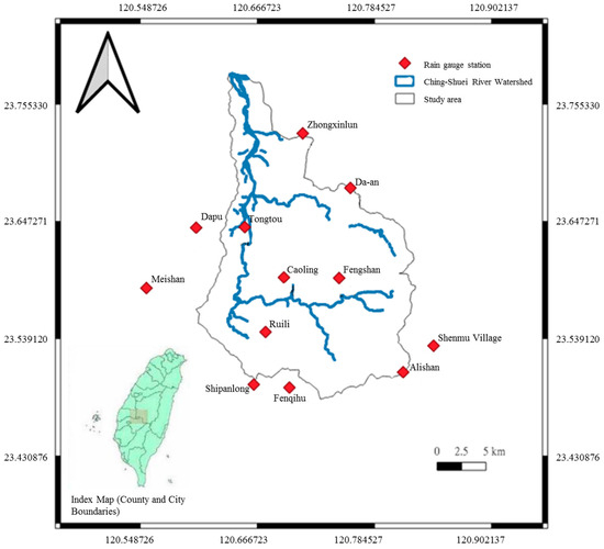
Figure 1.
Geographical location of the Ching-Shuei River watershed. Central Weather Administration. Available online: https://www.cwa.gov.tw/eng/ (accessed on 5 January 2024).
The Ching-Shuei River catchment area encompasses approximately 422 square kilometers. Its highest elevation is just under 2660 m, and its lowest is about 54 m. Figure 2 indicates how elevation is distributed across the area.
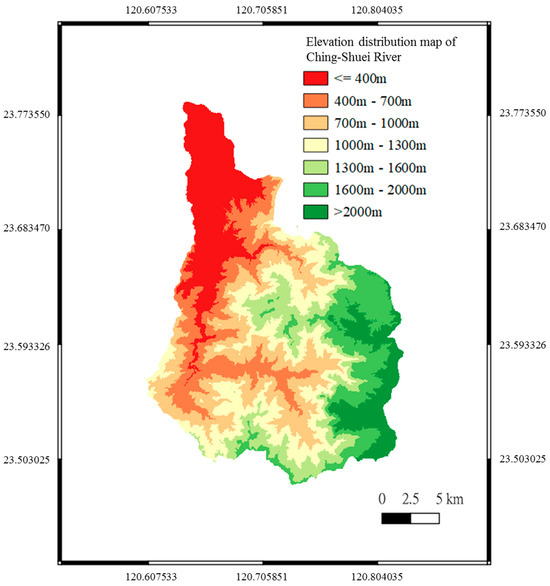
Figure 2.
Elevation distribution map of the Ching-Shuei River’s watershed. Geological Survey and Mining Management Agency, Ministry of Economic Affairs. Available online: https://www.gsmma.gov.tw/nss/p/index (accessed on 5 January 2024).
This paper’s primary research objects are the Ching-Shuei River watershed’s potential debris-flow streams, of which there are 33 (Bureau of Soil and Water Conservation, 2019), as shown in Figure 3.
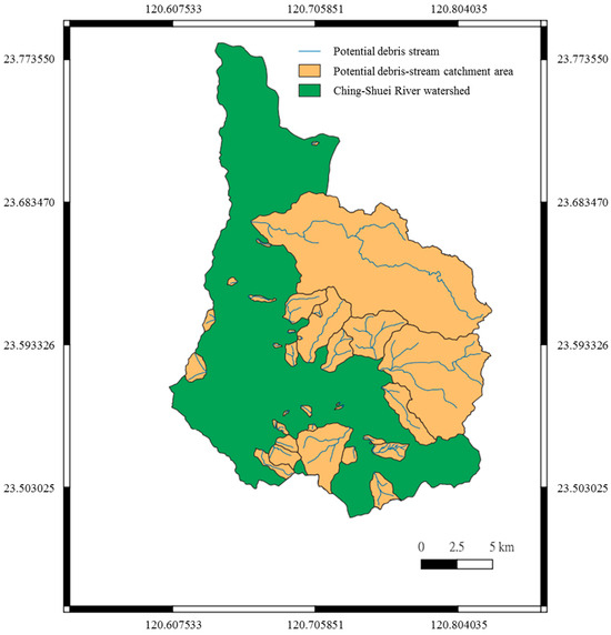
Figure 3.
Distribution map of potential streams and catchment areas. Agency of Rural Development and Soil and Water Conservation, MOA. Available online: https://www.ardswc.gov.tw/Home/eng/ (accessed on 5 January 2024).
The distribution of measurement stations around the catchment region of each debris-flow potential stream is depicted in Figure 4, and the reference rainfall stations of each debris-flow potential stream are used in this study.
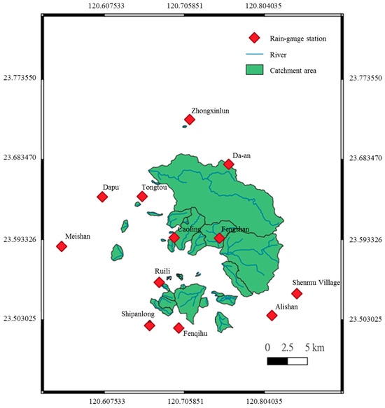
Figure 4.
Distribution map of potential debris streams and their catchment areas. Agency of Rural Development and Soil and Water Conservation, MOA. Available online: https://www.ardswc.gov.tw/Home/eng/ (accessed on 5 January 2024).
2.2. Research Methods
The following four subsections provide information on how the researchers collected and organized the information needed to characterize the impact variables of the 33 potential debris-flow streams.
Data Collection
Digital terrain model. A digital terrain model (DTM) of the focal geographical area was provided by Taiwan’s Ministry of the Interior (2016) via its open-government data platform. It has a data resolution of 20 × 20 m.
Geological map. Taiwan’s open-data platform also includes a 1:250,000 regional geological digital map of Taiwan prepared by the Central Geological Survey Institute of the Ministry of Economic Affairs (2013). The geological data for this study was derived from that map.
Satellite imagery. National Central University’s Center for Space and Remote Sensing Research, which has a 12.5 m × 12.5 m analytical imaging capacity, was the source for this paper’s satellite photographs. The photos analyzed included ones taken before and after the typhoons Mindulli (15 January–18 October 2004), Sinlaku (9 March–12 November 2008), and Morakot (12 April–1 November 2009) and before and after the torrential rains of 3 May 2012 (i.e., 16 February–26 October 2012) and 1 June 2017 (i.e., 28 January–17 November 2017).
Rainfall data. The Department of Atmospheric Sciences at Chinese Culture University maintains an Atmospheric Hydrology Research Database (2004–2017), which was the source of this paper’s rainfall information. After collection, the data required for this research were trimmed and screened using a rain field.
2.3. Judgment of Debris Flows Based on Satellite Images
To make it easier to nest with the potential debris-flow catchment areas for further study, the data generated from Satellite Pour l’Observation de la Terre (SPOT) pictures also include (1) the average Normalized Difference Vegetation Index (NDVI) before the incident of interest and (2) the size of the damage to the catchment area.
The SPOT satellite image data used in this study were obtained from the Center for Space and Remote Sensing Research at National Central University. The researchers also collected historical data on typhoons in the Ching-Shuei River watershed, which produced at least 40 mm of rain in one hour and/or 200 mm in 24 h, as determined by the Central Weather Bureau of Taiwan’s Ministry of Transportation and Communications. Figure 5 and Figure 6 show photos that were used in this research after screening in combination with the above-mentioned SPOT images.
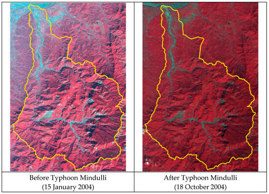
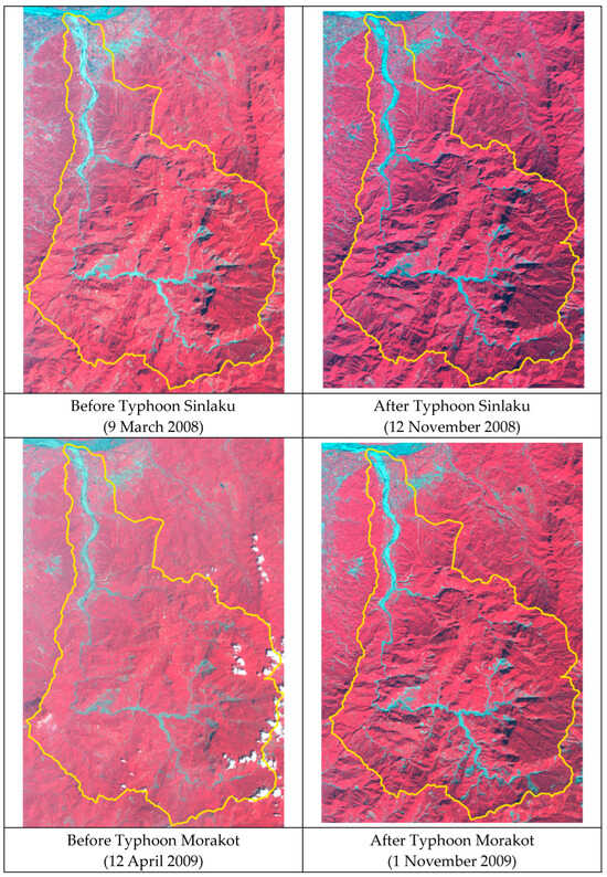
Figure 5.
Pairs of satellite images from before and after the three typhoons of interest.
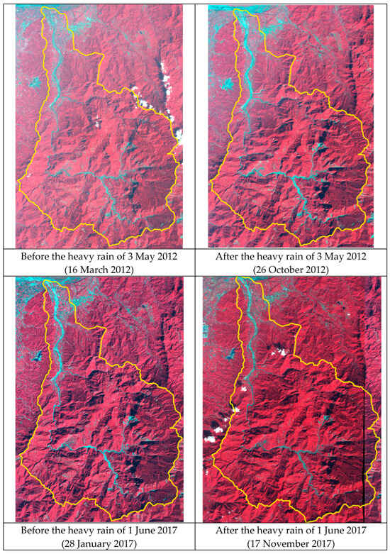
Figure 6.
Pairs of satellite images from before and after two non-typhoon-related instances of heavy rainfall.
2.4. Interpretation of Debris Flows
The more red light that green plants absorb and the more near-infrared light they reflect, the greater the difference between red light and near-infrared light. This enables us to compute an NDVI value ranging from −1 to +1 as follows:
where NIR is the near-infrared light band’s reflection intensity, and IR is the red light band’s reflection intensity. If NDVI is less than zero, non-vegetation features, including the cloud layer, surface water, roads, and buildings, are typically responsible. Thus, a higher NDVI equates to greener biomass being present.
In this study, the NDVI value of each phase of the image was calculated using QGIS 3.20 software’s raster-calculator tool. Figure 7 and Figure 8 graphically represent NDVI changes for each event of interest.
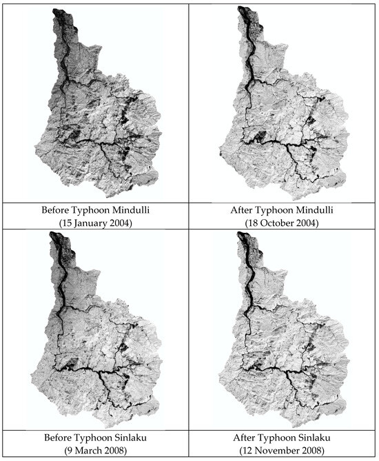
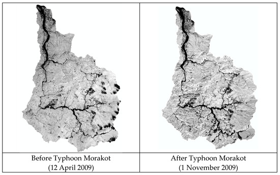
Figure 7.
Changes in vegetation cover before and after the three typhoons of interest.
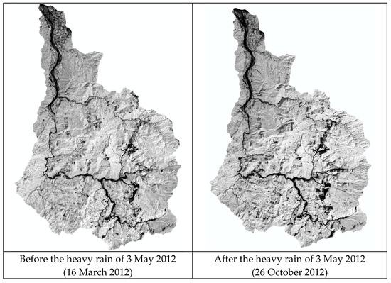
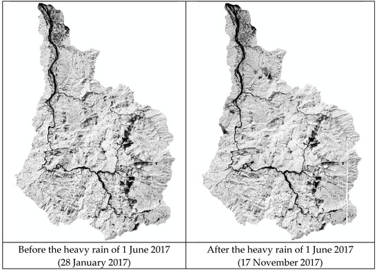
Figure 8.
Vegetation cover before and after two non-typhoon-related instances of heavy rainfall.
To determine whether a given event caused a landslide, we recorded the NDVI values prior to and following the incident and computed the average NDVI value prior to the event for the whole affected area. Then, to eliminate most landslide occurrences, they filtered out slopes of less than 30 degrees and subtracted post-event NDVI from pre-event NDVI (Figure 9). Next, they found relevant NDVI differences by superimposing QGIS and SPOT images (Figure 10 and Figure 11).
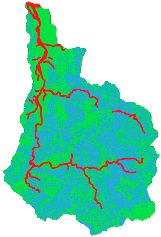
Figure 9.
The study area with waterways is shown in red, areas with slopes greater than 30 degrees in blue, and areas with slopes less than 30 degrees in green.
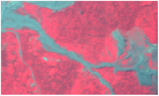
Figure 10.
Satellite image of debris flow DF041 caused by Typhoon Morakot.
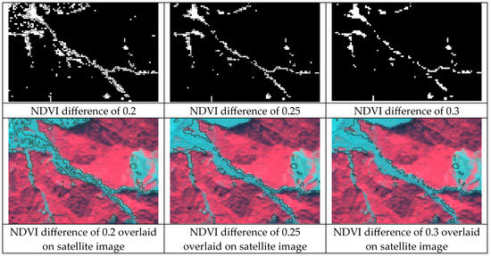
Figure 11.
Judgment-potential diagramming of debris flow DF041.
When the NDVI difference is 0.2, coverage is excessive. When it is 0.25, most of the landslides or riverbank erosion in satellite images are covered, and when the NDVI difference is 0.3, fewer areas are left uncovered. The difference in NDVI was 0.25, which is in the range of 0.2 and 0.3. Because a more cautious estimate was used in this investigation, the NDVI difference of 0.25 is more constant. Those landslides or riverbanks having a length of more than 200 m (10 grids) in the indicated potential valley and/or visible debris flows and alluvial fans were defined as debris-flow events.
2.5. Statistics, Test Screening, and Analysis of Geographical Factors
All 33 potential debris-flow catchment areas in the Ching-Shuei River watershed were examined using SPOT satellite images taken before and after five rainfall events that occurred between 2004 and 2017. This yielded a total of 165 occurrences and non-occurrences as samples for analysis, which became the basis for the researchers’ database of geophysical parameters.
2.5.1. Database Generated from Digital Terrain Model Data: Topographic Factors
The selection of factors likely to influence debris flows’ commencement was based on previous studies [9,12,35,37,38,39], as well as on the researchers’ prior knowledge of the causes of debris flows in the study area. Using the QGIS nesting approach, they created a unique terrestrial factor database for each of the 33 potential debris-flow streams comprising its total area, average slope, length, average slope of the stream bed, and shape coefficient, among other variables. The calculation of each such variable is explained, in turn, below.
Total area of catchment (A, unit: m2). The area of a given subdivision of the whole river catchment area pertinent to a particular potential debris flow is calculated as follows:
where a is the area of the grid in m2, and n is the number of grids the catchment subdivision contains.
A = a × n × 10−6,
Average slope of the catchment (S, unit: degrees). The average slope of a given potential debris flow’s catchment area is computed as follows:
where slope is the slope value of each of its grids.
Length (L, unit: m). The ArcMap program was used to nest the DTM with each potential debris-flow stream’s catchment area. Then, using hydrological analysis, its length was established by adding the number of connected grids as follows:
where n is the number of grids, and W is the width of the grid in m.
L = n × W,
Average slope of the stream bed (S, unit: degrees). The average slope of each potential debris-flow stream bed is computed as follows:
where H is the difference between the upstream elevation and the downstream elevation, in m, and L is the stream’s length.
S = tan − 1 (HL),
Shape coefficient (F). The shape coefficient of a given potential debris-flow stream is calculated as the ratio of its length to the width of its watershed, i.e.,
where A is the total area of its catchment in m2, and L is its length in m.
2.5.2. Values of the Selected Topographic Factors
As noted above, our data contained a total of 165 opportunities for a debris flow to have occurred in a potential debris-flow stream, i.e., five weather events ×33 catchments. Table 1 presents the minimum, maximum, and mean values of each terrestrial factor across those 165 debris-flow opportunities, along with their standard deviations (SDs).

Table 1.
Values and standard deviations of topographic factors for all 33 potential debris-flow areas.
2.5.3. Correlation Test of Topographic Factors
A Pearson correlation coefficient test was run following the computation of the topographic factors. Table 2 shows the resulting correlation matrix of the five topographic factors after normalization. In such a matrix, a correlation is considered significant if its absolute value is larger than 0.7, moderately significant if it is between 0.3 and 0.7, and marginally significant if it is below 0.3.
Table 2.
Pearson correlation coefficients for the topographic factors.
Catchment size was so strongly correlated to stream length that the researchers elected to omit the latter from further analyses. The remaining four topographic factors, however, could be deemed independent of one another because their eigenvalues were all less than 0.7, and all were, therefore, retained.
2.6. Database Generated from Digital Geological Maps and SPOT Satellite Images: Material Factors
Distance from faults and type of stratum are the two key components of the database the researchers created based on a digital geological map. Identifications of the catchment areas with the strongest potential for debris flows were statistically analyzed following Wu and Chen’s [40] grading criteria.
2.6.1. Geological Materials: Type of Stratum
Figure 12 shows the scale of the geological map used in this study, and Table 3 lists the scoring criteria. A stratum score is higher if the associated debris-flow ratio is higher and indicates that the stratum is more brittle; conversely, a lower stratum score means the stratum is stronger. After calculating those scores, the researchers conducted a nesting study using QGIS aimed at assessing each catchment area’s potential for debris flows. The types of strata in each potential debris-flow catchment area were obtained after the data had been sorted, and such flows were then estimated based on the proportion of each stratum to the area of the catchment area according to its weight, summarized. and counted.
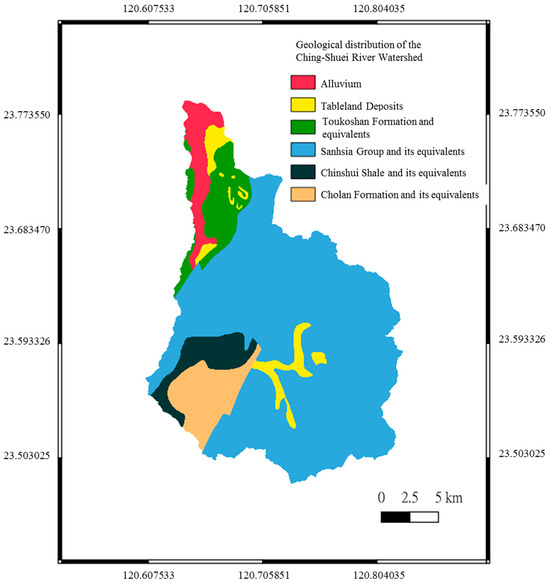
Figure 12.
Geological map of the Ching-Shuei River watershed. Geological Survey and Mining Management Agency, Ministry of Economic Affairs. Available online: https://www.gsmma.gov.tw/nss/p/index (accessed on 5 January 2024).
Table 3.
Stratum scoring criteria [40].
2.6.2. Geological Structure: Distance from the Region’s Central Fault
Distance from the nearest part of the geological fault system that runs through the centroid of the study area serves as this research’s primary geological structure variable. Figure 13 illustrates the fault system, and Table 4 presents the researchers’ scoring criteria. Scores increase and decrease according to proximity to the defect, with greater proximity being reflected in a higher score. The researchers calculated the distances from the faults in each catchment area separately and then totaled and tallied them before analyzing this information in light of the Ching-Shuei River watershed’s previously calculated debris-flow potential.
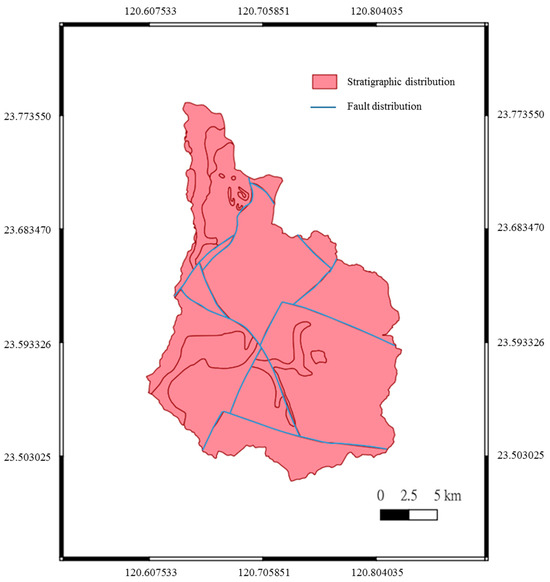
Figure 13.
Distribution of geological faults in the Ching-Shuei River watershed. Geological Survey and Mining Management Agency, Ministry of Economic Affairs. Available online: https://www.gsmma.gov.tw/nss/p/index (accessed on 5 January 2024).
Table 4.
Scoring criteria for fault assessment [40].
Two material factors, type of stratum and distance from a fault, were statistically evaluated for each of the 33 catchment areas and 165 occurrences of heavy rains. The results are presented in Table 5.
Table 5.
Values of material factors for all 33 catchment areas.
2.7. Processing and Collection of Rainfall Data: Trigger Factors
Rainfall is an important debris-flow initiator. The researchers, therefore, gathered rainfall data from 2004 to 2017, as well as SPOT images from each time period, to choose an appropriate event and then established each such event’s rainfall statistics. Figure 14 shows the locations of the 12 rain gauge stations that were used for that purpose.
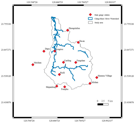
Figure 14.
Location map of rainfall stations. Central Weather Administration. Available online: https://www.cwa.gov.tw/eng/ (accessed on 5 January 2024).
Rainfield Cutting
As shown in Table 6, rainfield cutting comprises a set of methods that are used to make sense of the relationship between data from major rainfall events and slope damage [41]. In this study, Method 5 was adopted for the division of the rainfields. This was because Methods 1, 2, and 4 cut rainfields into time periods that are too long, thus artificially reducing their average intensity value, while Method 3 errs in the opposite direction, making some rainfall data too easy to ignore. Of Methods 5 and 6, the latter has a longer delay time, which also reduces the apparent average intensity of rainfall.
Table 6.
The six rainfield-cutting methods.
Because their centers were dispersed, the temporal and spatial distributions of the rainfall events in each of the 12 above-mentioned rain gauge stations’ records were inconsistent with one another. Therefore, the structural properties of the known spatial distribution of observed values are used in an approach known as kriging, which provides estimations closer to real-world events than conventional estimation techniques do.
After classifying each event’s rainfall, a Pearson correlation-coefficient test was run. Table 7 shows the correlation matrix among the various debris flows following the normalization of four separate sets of rainfall data. The eigenvalues for cumulative rainfall, maximum daily rainfall, and rainfall intensity (RI) are all greater than 0.7, demonstrating a strong correlation between these three factors. Maximum hourly rainfall can only be determined after a rainfall event has ended; however, the cumulative rainfall and rainfall intensity, which also have a significant impact on debris flows, can be computed while a rainfall event is still in progress. Extrapolating maximum daily rainfall from cumulative rainfall is quicker and more practical than measuring maximum daily rainfall directly. Therefore, using the maximum daily and hourly rainfall of the event as the key debris-flow triggers is more in line with the primary goal of this study: developing a basis for a real-time early warning of such flows. Table 8, Table 9 and Table 10 display the maximum daily rainfall and maximum hourly rainfall associated with each of the focal rainfall events. Rainfall distribution maps based on those data (Figure 15 and Figure 16) were then created in QGIS using the kriging algorithm.
Table 7.
Pearson correlation coefficients.
Table 8.
Rainfall data from the typhoons Mindulle and Sinlaku.
Table 9.
Rainfall data for Typhoon Morakot and the heavy rain of 3 May 2012.
Table 10.
Rainfall data from the heavy rain of 1 June 2017.
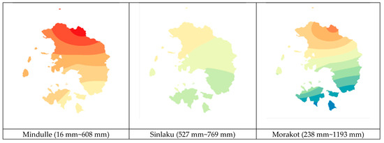
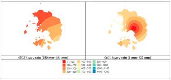
Figure 15.
Daily rainfall distribution map.
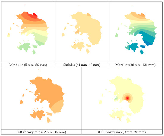

Figure 16.
Hourly rainfall distribution map.
2.8. Instability Index Method
The scores of each variable of the method have been standardized to provide a more objective statistical method of weighting the variables, which is defined by the formula Dtotal = D1W1 × D2W2 × D3W3 … × DnWn⋯(D1, D2, and Dn represent the indeterminate index value of each evaluation variable, such as slope, elevation, fault variable, etc. W1, W2, and Wn represent the weight value of the variables, and D_total represents the sensitivity of the occurrence of the potential area of geotechnical flow after summing up each variable.)
2.9. Rogers Regression
The Rogers Regression analysis is the odds ratio Odds = P/(1 − P), which is the probability of failure of the geotechnical potential zone (Y = 1) divided by the probability of no failure of the geotechnical potential zone (Y = 0), with P being the probability of failure of the geotechnical potential zone with a value between 0 and 1. P is the likelihood of failure of the geotechnical potential area, with a value between 0 and 1. Therefore, the odds ratio from 0 to 1 (P from 0 to 0.5) indicates a low probability of failure in the geotechnical potential zone (P = 0.5 implies the same probability of occurrence and non-occurrence of failure in the geotechnical potential zone) [42].
2.10. Artificial Neural Network
Artificial neural network is an information system modeled after biological neural transmission. It can obtain relevant information (input) from external or other artificial neurons, output it to external or other artificial neurons (output), and then operate it to build a system model (and the relationship between output and input), which can be used for prediction, decision-making, and judgment. The regression formulas in common regression analysis are also built using a set of samples, so neural networks can also be regarded as a special statistical technique.
The classification error matrix and the ROC (receiver operating characteristic, ROC) curve are the general methods for evaluating a model’s strengths and weaknesses [43,44,45,46]. Lee and Fei (2011) pointed out that the error matrix needs to be categorized with the help of clear categorization of landslide potential areas (e.g., artificially defining those above a certain value as belonging to the collapse group of a geotechnical potential area and those below a certain value as being in the non-collapse group of a geotechnical potential area) [39]. According to Gorsevski et al. (2006), the ROC curve is a graphical representation of the accuracy of the predicted probability, and the use of the area under the curve (AUC) under the ROC curve facilitates the measurement of the overall model fitness and the comparison between different models [46]. In addition, the ROC curve is plotted by the ability to explain the failure of the geotechnical potential zone with successive sensitivity values, and there is no need for artificial boundaries between the failure and non-failure classification of the geotechnical potential zone, so it is more suitable for the evaluation of the advantages and disadvantages of the failure sensitivity model of the geotechnical potential zone.
3. Results and Discussion
3.1. Judgment Results, Instability Index Method
The main objectives of this study’s analyses were (1) to assess variability in each debris-flow risk factor, (2) calculate the values of prediction for each of the potential debris flows, (3) assign impact weightings in accordance with the magnitude of the variation value, and (4) assign a score value and weights to each risk factor. In addition, the slope instability index Dt (Equation (7)) was presented as a highly flexible mathematical model for statistical measurement. It was computed as follows:
where is the shape coefficient, F is the distance from a fault, is the total area of the catchment, D is the strata type, is the average slope of the catchment area, is the maximum daily rainfall, is the average slope of the stream bed, and is the maximum hourly rainfall.
The upper- and lower-interval statistical methods were used to classify this study’s observations as a means of verifying its debris-flow prediction model’s probability of yielding misjudgments. The grading and scoring results of each factor were used as an independent variable matrix and were included in the slope-instability index of Equation (7). The results are displayed in Table 11. Stability index analysis of the model’s training sample showed to have an interpretation accuracy rate of 67.8%, and the parallel figure for its validation sample was 78.7%, equating to an overall interpretation accuracy rate of 70.9%.
Table 11.
Instability index analysis and judgment results.
By analyzing the landslide potential factor of the Ching-Shuei River using the instability index method, it was found that the advantage of the instability index method was that it could understand the landslide susceptibility zones of the landslide potential factor in detail and assign corresponding scoring values to understand the degree of impact on the catchment area of each grade distance of the collapse potential factor, and its disadvantage lied in that its weighting value was easily affected by the grade distance of the assessment process. The weights of the instability index method were obtained by dividing the standard deviation of each potential factor by the coefficient of variation of the mean. The process of finding the appropriate level of spacing of a potential factor will affect the standard deviation of the factor and the degree of importance of the factor in the subsequent evaluation, and the instability index method utilizes the linear superposition method of calculation [40,47,48]. The calculation process amplifies the influence of potential factors with high weighting values and reduces the influence of potential factors with low weighting values [49]. The results are similar to those of past scholars [49,50,51,52].
3.2. Judgment Results, Logit Regression
The same eight factors debris-flow variables were subjected to logit regression analysis according to the following two equations:
in which P is the likelihood that a debris flow will occur, L is the debris-flow factor resulting from Equation (8), and W is the regression coefficient. Table 12 shows the weight coefficients for each factor, and the polynomial resulting from the logit regression analysis is the following:
Table 12.
Coefficient table of the logit regression.
The likelihood value of a debris flow occurring was then obtained by substituting the results obtained from Equation (10) into Equation (8). If the value of P was greater than or equal to 0.5, it indicated that that such an event had happened. If P was smaller than 0.5, on the other hand, it had not happened. Table 13, which presents the researchers’ logit regression findings, shows that the validation sample’s interpretation accuracy rate was 83.0%, and that of the training sample was 79.7%, making for an overall interpretation-accuracy rate of 80.6%. The ratio of occurrence and non-occurrence in logit regression should ideally be 1:1, which could explain why its accuracy was not higher. Given the small number of debris-flow disasters relative to the number of rainfall events that could potentially trigger them, therefore, the difference in the parameters themselves is larger, so its correct interpretation is worse.
Table 13.
Logit regression analysis and judgment results.
By analyzing the slope potential factors of the Ching-Shuei River using Rogers regression, the relationship between the coefficients and landslide could be understood through the positive and negative coefficients, and the probability of collapse for each landslide potential factor could be known, which was equivalent to the coefficients of variability of the instability index method; however, the disadvantage was that the coefficients obtained from the analysis were susceptible to the influence of the selection of the data, which led to the results of the positive and negative coefficients of different values for the same rainfall conditions. The Rogers regression was obtained by multiplying the analyzed coefficients with the failure potential factors. Therefore, the number of potential failure factors analyzed after the Rogers regression was more than the coefficients obtained from the instability index analysis, which means that it magnified the extent of the impact of each failure potential factor on the slopes. Furthermore, Chan et al. (2015) mentioned that when the collapse catalog is plotted on extreme events, it tends to result in a lower importance of the potential factor [48]. Their results are similar to those of past scholars [48,49,53,54].
3.3. Judgment Results, Back-Propagation Neural Network
The same eight variables were normalized before being entered into IBM SPSS for back-propagation neural network analysis. The overall process of such analysis can be broken down into three parts, each of which is described in detail in its own subsection below.
3.3.1. Normalization of Debris-Flow Factors
Normalizing the input parameters prior to training increases both the accuracy and the efficiency of neural network learning and helps avoid convergence issues that might arise from the varying data ranges of the various debris-flow components [55]. The researchers primarily translated their data on the eight debris-flow factors from 0.1 to 0.9 using the mapping approach, i.e.,
where X represents the actual value, the actual value’s maximum value, and the actual value’s minimum value.
3.3.2. Back-Propagation Neural Network
This paper’s five focal weather events were entered into SPSS simultaneously for reverse-transfer neural network analysis, with 70% of the data used for training and 30% for verification. Table 14 presents the findings of such analysis. The verification sample’s interpretation accuracy rate was 91.5%, and that of the training sample was 94.1%, making for an overall accuracy of 93.3%. Table 15 shows the relative importance of each factor to accurate debris-flow disaster prediction.
Table 14.
Results of the analysis of the back-propagation neural network.
Table 15.
Results of the importance of the factors of the back-propagation neural network.
The back-propagation neural network predicted the potential area of slope disaster up to more than 90%, and the results were similar to those of past scholars [56,57,58].
3.4. Receiver Operating Characteristic Curves
A receiver operating characteristic (ROC) curve is a graphical analysis tool made up of a false-positive rate (FPR) on the x-axis and a true-positive rate (TPR) on the y-axis. Clarity and sensitivity are terms used to describe FPR and TPR, respectively. A binary classification model derives the coordinate points from the observed values and expected values of all samples. The ROC is situated in a square between 0 and 1 if the coordinate points are drawn on the x–y plane and connected with straight lines; during the judgment process, the space is divided into upper-left and lower-right blocks using the diagonal line from (0, 0) to (1, 1) as a reference line. As illustrated in Figure 17, an ROC curve’s classification result is better if it is above the diagonal line and travels to the upper left. Conversely, its classification result is worse if it is below the diagonal line.
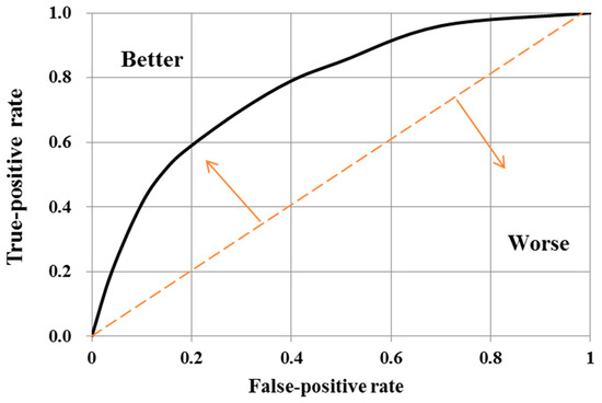
Figure 17.
Schematic diagram of the ROC curve.
The main output of ROC analysis is a binary classification model, such as occurred/not occurred. A threshold value is needed to define a continuous data output result. The following equations were used for calculating TPR and FPR:
where, as indicated in Table 16, TP and TN represent the correctness and error of interpretation, respectively.
Table 16.
Receiver operating characteristic curve evaluation form.
The area under the ROC curve, known as AUC, is a measure of how accurately landslides can be interpreted based on values that are observed and predicted. AUC’s value ranges from 0 to 1. The more AUC points there are, the more accurate the judgment. Perfect categorization is indicated by an AUC of 1. A model is considered to have no predictive value if its AUC is lower than 0.5, a fair predictive value if it is at least 0.5 but less than 0.7, a good predictive value if it is at least 0.7 but less than 0.9, and an excellent predictive value if 0.9 or higher.
The ROC curves for each type of analysis are shown in Figure 18, Figure 19 and Figure 20. Specifically, the AUC of the neural network was computed as 0.93, indicating this technique’s excellent ability to predict when a debris-flow disaster will occur. The AUC of logit regression analysis was 0.79, i.e., good, and that of the instability index method was 0.64, i.e., fair.
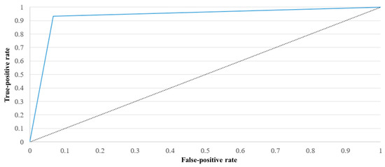
Figure 18.
Receiver operating characteristic curves for neural network analysis.
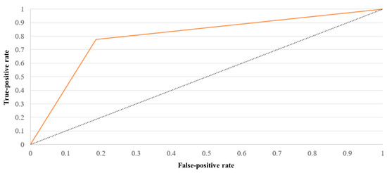
Figure 19.
Receiver operating characteristic curves for logit regression analysis.
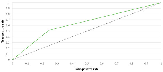
Figure 20.
Receiver operating characteristic curves for the instability index method.
As can be observed from the AUC area, all three models reached above 0.7, representing the ability to effectively predict the occurrence of a landslide in the Ching-Shuei River using the instability index, Rogers regression, and artificial neural network. By comparing the three methods of evaluating model accuracy, it could be found that the accuracy of the ROC curve was higher than that of the categorical error matrix. It is hypothesized that the reason for this is that the total accuracy of the model of the categorical error matrix is limited by the correct rate of the collapse and the correct rate of the non-landslide, and the difference in the number of base grids of the landslide and the non-landslide is very large, which then influences the subsequent calculation of the correct rate of the two and the total accuracy, respectively. In contrast, the ROC curve only considers the proportion of accurately misinterpreted versus accurately correct and plots them cumulatively so that the accuracy of the ROC curve is higher than that of the categorical error matrix for subsequent model accuracy comparisons.
4. Conclusions
In this study, an attempt was made to use the total area of catchment, average slope of the catchment, the length of the stream, the average slope of the stream bed, the shape coefficient, the type of stratum, the distance from the region’s central fault, and the trigger factors. The sensitivity analysis of the geotechnical potential zone was conducted by using eight variables, together with the instability index, Rogers regression, and neural network. The comparison of the results with those of previous studies revealed that the importance of the variables overlapped with each other, but nevertheless, the importance of the factors affecting the geotechnical potential zones would be different in different regions due to the different characteristics of the environments.
This paper’s evaluations of the instability index method, logit regression analysis, and neural network analysis as potential means of precisely predicting debris-flow disasters revealed that each has its benefits and drawbacks. The following conclusions can be drawn from the results. First, the three methods’ general accuracy rates ranged from 70.9% to 93.3%. When it came to the prediction of debris-flow disasters, however, the spread was much wider: 83.7% for neural networks, 48.1% for logit regression analysis, and 32.7% for instability index analysis. In predicting the absence of any debris-flow disaster, logit regression analysis performed best, at 98.4%; neural network analysis almost as well, at 97.4%; and the instability index method the least well, at 87.1%. According to neural network analysis, the three most important of the authors’ eight selected debris-flow triggers (in descending order of importance) were (1) total catchment area, (2) maximum hourly rainfall, and (3) average slope of the catchment, while the least important was the distance from a fault. This study’s AUC of the ROC curve results suggest that all three of the tested models can be used for this purpose but that the neural network has the best discrimination ability (i.e., excellent) and the instability index method the worst (i.e., fair).
Future researchers are encouraged to verify this paper’s results using data from weather events in other regions. Also, its list of potential factors that trigger debris flows should not be regarded as exhaustive. The future identification of other such factors would only tend to improve the performance of debris-flow prediction models. Additionally, the present work’s results suggest that when using the instability index method, the initial factor classification could usefully divide factors into more intervals, thereby improving the precision of its judgment of areas’ landslide potential. The accuracy of logit regression, meanwhile, would be improved if more debris flows were included to balance the number of cases with and without such flows. Lastly, this study did not include preservation objects such as residences and public infrastructure. Including them would enrich this line of research as a basis for future novel approaches to slope-disaster risk analysis.
Author Contributions
Conceptualization, J.-Y.L.; data curation, L.-K.Y.; writing—original draft, L.-K.Y.; writing—review and editing, J.-C.C.; supervision, J.-Y.L. All authors have read and agreed to the published version of the manuscript.
Funding
This research received no external funding.
Institutional Review Board Statement
Not applicable.
Informed Consent Statement
Not applicable.
Data Availability Statement
The original contributions presented in the study are included in the article, further inquiries can be directed to the corresponding author.
Acknowledgments
We would like to thank the anonymous reviewers for their helpful suggestions and feedback.
Conflicts of Interest
The authors declare no conflicts of interest.
References
- Dietrich, W.; Dunne, T. Sediment budget for a small catchment in a mountainous terrain. Zeits. Geomorphol. Supp. 1978, 29, 191–206. [Google Scholar]
- Hungr, O.; Evans, S.G.; Bovis, M.J.; Hutchinson, J.N. A review of the classification of landslides of the flow type. Environ. Eng. Geosci. 2001, 7, 221–238. [Google Scholar] [CrossRef]
- Corominas, J.; van Westen, C.; Frattini, P.; Cascini, L.; Malet, J.-P.; Fotopoulou, S.; Catani, F.; Van Den Eeckhaut, M.; Mavrouli, O.; Agliardi, F.; et al. Recommendations for the quantitative analysis of landslide risk. Bull. Eng. Geol. Environ. 2014, 73, 209–263. [Google Scholar] [CrossRef]
- Takahashi, T. Debris Flow: Mechanics, Prediction and Countermeasures, 1st ed.; Taylor & Francis: London, UK, 2007. [Google Scholar]
- Yang, Z.; Wang, L.; Qiao, J.; Uchimura, T.; Wang, L. Application and verification of a multivariate real-time early warning method for rainfall-induced landslides: Implication for evolution of landslide-generated debris flows. Landslides 2020, 17, 2409–2419. [Google Scholar] [CrossRef]
- Deng, Y.-C.; Hwang, J.-H.; Lyu, Y.-D. Developing real-time nowcasting system for regional landslide hazard assessment under extreme rainfall events. Water 2021, 13, 732. [Google Scholar] [CrossRef]
- Westra, S.J.; Fowler, H.J.; Evans, J.P.; Alexander, L.V.; Berg, P.R.; Johnson, F.; Kendon, E.J.; Lenderink, G.; Roberts, N.M. Future changes to the intensity and frequency of short-duration extreme rainfall. Rev. Geophys. 2014, 52, 522–555. [Google Scholar] [CrossRef]
- van Westen, C.J.; Castellanos, E.; Kuriakose, S.L. Spatial data for landslide susceptibility, hazard, and vulnerability assessment: An overview. Eng. Geol. 2008, 102, 112–131. [Google Scholar] [CrossRef]
- Nikolova, V.; Kamburov, A.; Rizova, R. Morphometric analysis of debris flows basins in the eastern Rhodopes (Bulgaria) using geospatial technologies. Nat. Hazards 2021, 105, 159–175. [Google Scholar] [CrossRef]
- Bovis, M.J.; Jakob, M. The role of debris supply conditions in predicting debris flow activity. Earth Surf. Process. Landf. 1999, 24, 1039–1054. [Google Scholar] [CrossRef]
- Melton, M.A. Correlation structure of morphometric properties of drainage systems and their controlling agents. J. Geol. 1958, 66, 442–460. [Google Scholar] [CrossRef]
- Wilford, D.J.; Sakals, M.E.; Innes, J.L.; Sidle, R.C.; Bergerud, W.A. Recognition of debris flow, debris flood and flood hazard through watershed morphometrics. Landslides 2004, 1, 61–66. [Google Scholar] [CrossRef]
- Lin, C.-W.; Liu, S.-H.; Lee, S.-Y.; Liu, C.-C. Impacts of the chi-chi earthquake on subsequent rainfall-induced landslides in central Taiwan. Eng. Geol. 2006, 86, 87–101. [Google Scholar] [CrossRef]
- Lin, C.-W.; Shieh, C.-L.; Yuan, B.-D.; Shieh, Y.-C.; Liu, S.-H.; Lee, S.-Y. Impact of chi-chi earthquake on the occurrence of landslides and debris flows: Example from the Chenyulan river watershed, Nantou, Taiwan. Eng. Geol. 2004, 71, 49–61. [Google Scholar] [CrossRef]
- Cui, P.; Chen, X.-Q.; Zhu, Y.-Y.; Su, F.-H.; Wei, F.-Q.; Han, Y.-S.; Liu, H.-J.; Zhuang, J.-Q. The Wenchuan earthquake (May 12, 2008), Sichuan province, China, and resulting geohazards. Nat. Hazards 2011, 56, 19–36. [Google Scholar] [CrossRef]
- Hu, K.; Cui, P.; You, Y.; Chen, X. Influence of debris supply on the activity of post-quake debris flows. Chin. J. Geol. Hazard Control 2011, 22, 1–6. [Google Scholar]
- Tang, C.; Zhu, J.; Li, W.L.; Liang, J.T. Rainfall-triggered debris flows following the Wenchuan earthquake. Bull. Eng. Geol. Environ. 2009, 68, 187–194. [Google Scholar] [CrossRef]
- Huang, R.; Fan, X. The landslide story. Nat. Geosci. 2013, 6, 325–326. [Google Scholar] [CrossRef]
- Cui, P.; Zhou, G.G.D.; Zhu, X.H.; Zhang, J.Q. Scale amplification of natural debris flows caused by cascading landslide dam failures. Geomorphology 2013, 182, 173–189. [Google Scholar] [CrossRef]
- Hürlimann, M.; Rickenmann, D.; Medina, V.; Bateman, A. Evaluation of approaches to calculate debris-flow parameters for hazard assessment. Eng. Geol. 2008, 102, 152–163. [Google Scholar] [CrossRef]
- Chang, M.; Tang, C.; Van Asch, T.W.J.; Cai, F. Hazard assessment of debris flows in the Wenchuan earthquake-stricken area, south west China. Landslides 2017, 14, 1783–1792. [Google Scholar] [CrossRef]
- He, Y.P.; Xie, H.; Cui, P.; Wei, F.Q.; Zhong, D.L.; Gardner, J.S. Gis-based hazard mapping and zonation of debris flows in Xiaojiang basin, southwestern China. Environ. Geol. 2003, 45, 286–293. [Google Scholar] [CrossRef]
- Berti, M.; Simoni, A. Prediction of debris flow inundation areas using empirical mobility relationships. Geomorphology 2007, 90, 144–161. [Google Scholar] [CrossRef]
- Rickenmann, D. Empirical relationships for debris flows. Nat. Hazards 1999, 19, 47–77. [Google Scholar] [CrossRef]
- Tang, C.; Zhu, J.; Chang, M.; Ding, J.; Qi, X. An empirical–statistical model for predicting debris-flow runout zones in the Wenchuan earthquake area. Quat. Int. 2012, 250, 63–73. [Google Scholar] [CrossRef]
- Hungr, O.; McDougall, S. Two numerical models for landslide dynamic analysis. Comput. Geosci. 2009, 35, 978–992. [Google Scholar] [CrossRef]
- Zhang, S.; Zhang, L.-M.; Chen, H.-X.; Yuan, Q.; Pan, H. Changes in runout distances of debris flows over time in the Wenchuan earthquake zone. J. Mt. Sci. 2013, 10, 281–292. [Google Scholar] [CrossRef]
- Liou, Y.-A.; Kar, S.K.; Chang, L. Use of high-resolution formosat-2 satellite images for post-earthquake disaster assessment: A study following the 12 May 2008 Wenchuan earthquake. Int. J. Remote Sens. 2010, 31, 3355–3368. [Google Scholar] [CrossRef]
- Tang Chuan, Z.J.; Wan, S.-Y.; Zhou, C.-H. Loss evaluation of urban debris flow hazard using high spatial resolution satellite imagery. Sci. Geogr. Sin. 2006, 26, 358–363. [Google Scholar]
- Chien-Yuan, C.; Tien-Chien, C.; Fan-Chieh, Y.; Wen-Hui, Y.; Chun-Chieh, T. Rainfall duration and debris-flow initiated studies for real-time monitoring. Environ. Geol. 2005, 47, 715–724. [Google Scholar] [CrossRef]
- Koi, T.; Hotta, N.; Ishigaki, I.; Matuzaki, N.; Uchiyama, Y.; Suzuki, M. Prolonged impact of earthquake-induced landslides on sediment yield in a mountain watershed: The Tanzawa region, Japan. Geomorphology 2008, 101, 692–702. [Google Scholar] [CrossRef]
- Ayalew, L.; Yamagishi, H. The application of Gis-based logistic regression for landslide susceptibility mapping in the Kakuda-Yahiko mountains, central Japan. Geomorphology 2005, 65, 15–31. [Google Scholar] [CrossRef]
- Das, I.; Sahoo, S.; van Westen, C.; Stein, A.; Hack, R. Landslide susceptibility assessment using logistic regression and its comparison with a rock mass classification system, along a road section in the northern Himalayas (India). Geomorphology 2010, 114, 627–637. [Google Scholar] [CrossRef]
- Shan, Y.; Chen, S.; Zhong, Q. Rapid prediction of landslide dam stability using the logistic regression method. Landslides 2020, 17, 2931–2956. [Google Scholar] [CrossRef]
- Wu, S.; Chen, J.; Zhou, W.; Iqbal, J.; Yao, L. A modified logit model for assessment and validation of debris-flow susceptibility. Bull. Eng. Geol. Environ. 2019, 78, 4421–4438. [Google Scholar] [CrossRef]
- Süzen, M.L.; Doyuran, V. Data driven bivariate landslide susceptibility assessment using geographical information systems: A method and application to asarsuyu catchment, Turkey. Eng. Geol. 2004, 71, 303–321. [Google Scholar] [CrossRef]
- Dias, V.; Vieira, B.; Gramani, M. Parâmetros morfológicos e morfométricos como indicadores da magnitude das corridas de detritos na serra do mar paulista. Confins 2016, 29, 1–29. [Google Scholar] [CrossRef]
- Kung, H.-Y.; Ku, H.-H.; Lin, C.-Y.; Tasi, K.-J. The design of numerical prediction models system for the debris-flow disaster in Taiwan. Chiao Da Mangement Rev. 2005, 25, 109–140. [Google Scholar] [CrossRef]
- Lee, C.-T.; Fei, L.-Y. Potential landslide and debris flow hazard prediction in the Lanyang river basin. J. Adv. Technol. Manag. 2011, 1, 67–83. [Google Scholar]
- Wu, C.H.; Chen, S.C. The evaluation of the landslide potential prediction models used in Taiwan. J. Soil Water Conserv. 2004, 36, 295–306. [Google Scholar]
- Jan, C.D.; Lee, M.H. A debris-flow rainfall-based warning model. J. Chin. Soil Water Conserv. 2004, 35, 275–285. [Google Scholar] [CrossRef]
- Dai, F.; Lee, C. A spatiotemporal probabilistic modelling of storm-induced shallow landsliding using aerial photographs and logistic regression. Earth Surf. Process. Landf. 2003, 28, 527–545. [Google Scholar] [CrossRef]
- Bui, D.T.; Lofman, O.; Revhaug, I.; Dick, O. Landslide susceptibility analysis in the Hoa Binh province of Vietnam using statistical index and logistic regression. Nat. Hazards 2011, 59, 1413–1444. [Google Scholar] [CrossRef]
- Chau, K.T.; Chan, J.E. Regional bias of landslide data in generating susceptibility maps using logistic regression: Case of Hong Kong island. Landslides 2005, 2, 280–290. [Google Scholar] [CrossRef]
- Chauhan, S.; Sharma, M.; Arora, M.K. Landslide susceptibility zonation of the chamoli region, garhwal Himalayas, using logistic regression model. Landslides 2010, 7, 411–423. [Google Scholar] [CrossRef]
- Gorsevski, P.V.; Gessler, P.E.; Foltz, R.B.; Elliot, W.J. Spatial prediction of landslide hazard using logistic regression and roc analysis. Trans. GIS 2006, 10, 395–415. [Google Scholar] [CrossRef]
- Su, M.-B.; Tsai, H.-S.; Jien, L.-B. Quantitative assessment of hillslope stability in a watershed. J. Chin. Soil Water Conserv. 1998, 29, 105–114. [Google Scholar] [CrossRef]
- Chan, H.-C.; Tsai, P.-S.; Chang, C.-C.; Huang, W.-J.; Wu, J.-J. Vegetation recovery on landslide susceptibility in the chi-sun watershed. J. Chin. Soil Water Conserv. 2015, 46, 47–60. [Google Scholar] [CrossRef]
- Hung, C.-Y.; Lin, H.-M. Comparison of mass wasting susceptibility evaluation for haiduan township in taitung county: Logistic regression and instability index. Bull. Geogr. Soc. China 2012, 77–103. [Google Scholar] [CrossRef]
- Yang, M.-D.; Huang, Y.-D.; Huang, K.-H.; Chang, Y.-H. Landslide hazard evaluated by a landslide susceptibility map-a case study of Chenyulan river basin. J. Chin. Soil Water Conserv. 2012, 43, 1–11. [Google Scholar] [CrossRef]
- Hsieh, Y.-T.; Chen, J.-C.; Huang, Y.-L.; Chung, Y.-L.; Chen, C.-T.; Wu, S.-T. Application of the digital aerial images for landslide monitoring and susceptibility mapping: A case study of Guangao area. J. Slopeland Hazard Prev. 2014, 13, 14–29. [Google Scholar]
- Huang, Y.-N.; Yeh, C.-H. Modeling and analysis of landslide potential for Alishan mountain road in southwestern Taiwan. J. Chin. Soil Water Conserv. 2020, 51, 55–64. [Google Scholar] [CrossRef]
- Chen, S.-C.; Ferng, J.-W. The application of logistic regression for landslide susceptibility mapping in the Jhuoshuei river basin. J. Chin. Soil Water Conserv. 2005, 36, 191–201. [Google Scholar] [CrossRef]
- Lee, J.-T.; Chang, C.-C.; Chan, H.-C.; Laio, P.-Y.; Hung, Y.-J. The application of logistic regression for landslide susceptibility analysis-a case study in Alishan area. J. Chin. Soil Water Conserv. 2012, 43, 167–176. [Google Scholar] [CrossRef]
- Hsein Juang, C.; Chen, C.J. A rational method for development of limit state for liquefaction evaluation based on shear wave velocity measurements. Int. J. Numer. Anal. Methods Geomech. 2000, 24, 1–27. [Google Scholar] [CrossRef]
- Alqhtani, S.M. Flidnd-mcn: Fake label images detection of natural disasters with multi model convolutional neural network. J. Intell. Fuzzy Syst. 2022, 43, 7081–7095. [Google Scholar] [CrossRef]
- Nisa, A.K.; Irawan, M.I.; Pratomo, D.G. Identification of potential landslide disaster in east java using neural network model (case study: District of Ponogoro). J. Phys. Conf. Ser. 2019, 1366, 012095. [Google Scholar] [CrossRef]
- Pradhan, B.; Lee, S. Landslide susceptibility assessment and factor effect analysis: Backpropagation artificial neural networks and their comparison with frequency ratio and bivariate logistic regression modelling. Environ. Model. Softw. 2010, 25, 747–759. [Google Scholar] [CrossRef]
Disclaimer/Publisher’s Note: The statements, opinions and data contained in all publications are solely those of the individual author(s) and contributor(s) and not of MDPI and/or the editor(s). MDPI and/or the editor(s) disclaim responsibility for any injury to people or property resulting from any ideas, methods, instructions or products referred to in the content. |
© 2024 by the authors. Licensee MDPI, Basel, Switzerland. This article is an open access article distributed under the terms and conditions of the Creative Commons Attribution (CC BY) license (https://creativecommons.org/licenses/by/4.0/).